- Trang chủ >>
- Khoa Học Tự Nhiên >>
- Vật lý
lecture notes on quantum mechanics
Bạn đang xem bản rút gọn của tài liệu. Xem và tải ngay bản đầy đủ của tài liệu tại đây (2.71 MB, 265 trang )
LECTURE NOTES
ON QUANTUM MECHANICS
Dr. Shun-Qing Shen
Department of Physics
The University of Hong Kong
September 2004
Con ten ts
0.1 GeneralInformation ix
1 Fundamental Concepts 1
1.1 Relation between experimental interpretations and theoretical inferences . . . 2
1.2 MaterialsfromBritannicaOnline 3
1.2.1 Photoelectric eect 3
1.2.2 Frank-Hertzexperiment 5
1.2.3 Compton eect 6
1.3 TheStern-GerlachExperiment 7
1.3.1 TheStern-Gerlachexperiment 7
1.3.2 SequentialStern-GerlachExperiment 9
1.3.3 AnalogywithPolarizationofLight 11
1.4 DiracNotationandOperators 11
1.5 BaseketsandMatrixRepresentation 14
1.5.1 EigenketsofanObservable 14
1.5.2 EigenketsasBasekets: 15
1.5.3 MatrixRepresentation: 16
1.6 Measurements,Observables&TheUncertaintyRelation 18
ii
CONTENTS – MANUSCRIPT
1.6.1 Measurements 18
1.6.2 Spin1/2system 19
1.6.3 ProbabilityPostulate 20
1.6.4 S
{
and S
|
21
1.6.5 TheAlgebraofSpinOperators 23
1.6.6 Observable 24
1.7 ChangeofBasis 26
1.7.1 Transformation Operator 27
1.7.2 TransformationMatrix 28
1.7.3 Diagonalization 30
1.8 Position,Momentum,andTranslation 31
1.8.1 ContinuousSpectra 31
1.8.2 Some properties of the function 32
1.8.3 PositionEigenketsandPositionMeasurements 33
1.8.4 Translation 34
1.9 TheUncertaintyRelation 38
2 Quantum Dynamics 46
2.1 TimeEvolutionandtheSchrödingerEquation 46
2.1.1 TimeEvolutionOperator 46
2.1.2 TheSchrodingerEquation. 48
2.1.3 TimeDependenceofExpectationValue:SpinPrecession. 52
2.2 TheSchrodingerversustheHeisenbergPicture 54
2.2.1 Unitaryoperators 54
2.2.2 TwoApproaches 55
iii
CONTENTS – MANUSCRIPT
2.2.3 TheHeisenbergEquationofMotion 56
2.2.4 HowtoconstructaHamiltonian 57
2.3 SimpleHarmonicOscillator 59
2.3.1 Eigenvalueandeigenstates 59
2.3.2 Time Development of the Oscillator . . 66
2.3.3 TheCoherentState 67
2.4 SchrodingerWaveEquation:SimpleHarmonicOscillator 68
2.5 Propagators and Feynman Path Integrals . . . 70
2.5.1 Propagators in Wave Mechanics. 70
2.5.2 Propagator as a Transition Amplitude. . 75
2.6 TheGaugeTransformationandPhaseofWaveFunction 79
2.6.1 ConstantPotential 79
2.6.2 GaugeTransformationinElectromagnetism 81
2.6.3 TheGaugeTransformation 84
2.6.4 The Aharonov-Bohm Eect 86
2.7 InterpretationofWaveFunction. 88
2.7.1 What’s
({)? 88
2.7.2 TheClassicalLimit 90
2.8 Examples 91
2.8.1 Onedimensionalsquarewellpotential 91
2.8.2 A charged particle in a uniform magnetic field . . . 95
3 Theory of Angular Momentum 98
3.1 RotationandAngularMomentum 98
3.1.1 Finite versus infinitesimal rotation . . . 99
iv
CONTENTS – MANUSCRIPT
3.1.2 Orbitalangularmomentum 104
3.1.3 Rotationoperatorforspin1/2 106
3.1.4 Spin precession revisited . 107
3.2 RotationGroupandtheEulerAngles 108
3.2.1 TheGroupConcept 108
3.2.2 Orthogonal Group 109
3.2.3 “Special”? 110
3.2.4 UnitaryUnimodularGroup 110
3.2.5 EulerRotations 112
3.3 EigenvaluesandEigenketsofAngularMomentum 114
3.3.1 RepresentationofRotationOperator 120
3.4 SchwingerOscillatorModel 121
3.4.1 Spin1/2system 125
3.4.2 Two-spin—1/2 system . . 126
3.4.3 ExplicitFormulaforRotationMatrices. 128
3.5 Combination of Angular Momentum and Clebsh-Gordan Coe!cients 130
3.5.1 Clebsch-Gordan coe!cients 133
3.6 Examples 137
3.6.1 Twospin-1/2systems 137
3.6.2 Spin-orbitcoupling 137
4 Symmetries in Physics 140
4.1 SymmetriesandConservationLaws 141
4.1.1 SymmetryinClassicalPhysics 141
4.1.2 SymmetryinQuantumMechanics 142
v
CONTENTS – MANUSCRIPT
4.1.3 Degeneracy 143
4.1.4 Symmetryandsymmetrybreaking 144
4.1.5 Summary:symmetriesinphysics 147
4.2 DiscreteSymmetries 148
4.2.1 Parity 148
4.2.2 TheMomentumOperator 150
4.2.3 TheAngularMomentum 151
4.2.4 LatticeTranslation 154
4.3 PermutationSymmetryandIdenticalParticles 157
4.3.1 Identicalparticles 157
4.4 TimeReversal 162
4.4.1 Classicalcases 162
4.4.2 Antilinear Operators . . . 162
4.4.3 Antiunitaryoperators 162
4.4.4 Tforazerospinparticle 162
4.4.5 Tforanonzerospinparticle 162
5 Approximation Methods for Bound States 163
5.1 TheVariationMethod 163
5.1.1 Expectationvalueoftheenergy 164
5.1.2 Particle in a one-dimensional infinite square well . . 165
5.1.3 GroundStateofHeliumAtom 166
5.2 StationaryPerturbationTheory:NondegenerateCase 168
5.2.1 StatementoftheProblem 168
5.2.2 TheTwo-StateProblem 169
vi
CONTENTS – MANUSCRIPT
5.2.3 Formal Development of Perturbation··· 170
5.3 ApplicationofthePerturbationExpansion 174
5.3.1 Simpleharmonicoscillator 174
5.3.2 Atomichydrogen 177
5.4 StationaryPerturbationTheory: DegenerateCase 179
5.4.1 Revisitedtwo-stateproblem 180
5.4.2 Thebasicprocedureofdegenerateperturbationtheory 181
5.4.3 Example: Zeeman Eect 183
5.4.4 Example: First Order Stark EectinHydrogen 184
5.5 TheWentzel-Kramers-Brillouin(WKB)approximation 186
5.6 Time-dependent Problem: Interacting Picture and Two-State Problem . . . . 186
5.6.1 Time-dependentPotentialandInteractingPicture 187
5.6.2 Time-dependentTwo-StateProblem 188
5.7 Time-dependentPerturbationProblem 191
5.7.1 PerturbationTheory 191
5.7.2 Time-independentperturbation 193
5.7.3 Harmonicperturbation 193
5.7.4 TheGoldenRule 194
6 Collision Theory 196
6.1 Collisions in one- and three-dimensions 197
6.1.1 One-dimensionalsquarepotentialbarriers 197
6.2 Collision in three dimensions . . 200
6.3 ScatteringbySphericallySymmetricPotentials 204
6.4 Applications 209
vii
CONTENTS – MANUSCRIPT
6.4.1 Scatteringbyasquarewell 209
6.4.2 Scatteringbyahard-spherepotential 211
6.5 Approximate Collision Theory . . 212
6.5.1 TheLippman-SchwingerEquation 212
6.5.2 TheBornApproximation 216
6.5.3 Application:fromYukawapotentialtoColoumbpotential 217
6.5.4 IdenticalParticlesandScattering 218
6.6 Landau-ZenerProblem 219
7SelectedTopics 220
7.1 QuantumStatistics 220
7.1.1 DensityOperatorandEnsembles 220
7.1.2 QuantumStatisticalMechanism 223
7.1.3 QuantumStatistics 226
7.1.4 Systemsofnon-interactionparticles 227
7.1.5 Bose-EinsteinCondensation 230
7.1.6 Freefermiongas 232
7.2 Quantum Hall Eect 233
7.2.1 Hall Eect 234
7.2.2 Quantum Hall Eect 236
7.2.3 Laughlin’sTheory 238
7.2.4 Charged particle in the presence of a magnetic field 240
7.2.5 Landau Level and Quantum Hall Eect 243
7.3 QuantumMagnetism 244
7.3.1 SpinExchange 245
viii
CONTENTS – MANUSCRIPT
7.3.2 Two-SiteProblem 247
7.3.3 Ferromagnetic Exchange (M?0) 249
7.3.4 AntiferromagneticExchange 251
0.1 General Information
• Aim/Following-up: The course provides an introduction to advanced techniques
in quantum mechanics and their application to several selected topics in condensed
matter physics.
• Contents: Dirac notation and formalism, time evolution of quantum systems, angu-
lar momentum theory, creation and annihilation operators (the second quantization
representation), symmetries and conservation laws, permutation symmetry and identi-
cal particles, quantum statistics, non-degenerate and degenerate perturbation theory,
time-dependent perturbation theory, the variational method
• Prerequisites: PHYS2321, PHYS2322, PHYS2323, and PHYS2325
• Co-requisite:Nil
• Teaching: 36 hours of lectures and tutorial classes
• Duration: One semester (1st semester)
• As sessment: One-three hour examination (70%) and course assessment (30%)
• Textb ook: J. J. Sakurai, Modern Quantum Mechanics (Addison-Wesley, 1994)
• Web page: All lectures notes in pdf files can
be download from the site.
ix
CONTENTS – MANUSCRIPT
• References:L.Schi, Quantum Mechanics (McGraw-Hill, 1968, 3nd ed.); Richard
Feynman, Robert B. Leighton, and Matthew L. Sands, Feynman Lectures on Physics
Vol. III, (Addison-Wesley Publishing Co., 1965); L. D. Landau and E. M. Lifshitz,
Quantum Mechanics
Time and Venue: Year 2004 (Weeks 2 — 14)
11:40 -12:30: Monday/S802
11:40 -12:30: Wednesday/S802
11:40 -12:30: Friday/S802
x
CONTENTS – MANUSCRIPT
Numerical values of some physical quantities
~ =1=054 × 10
27
erg-sec (Planck’s constant divided by 2
h =4=80 × 10
10
esu(magnitudeofelectroncharge)
p =0=911 × 10
27
g (electron mass)
P =1=672 × 10
24
g (proton mass)
d
0
= ~
2
@ph
2
=5=29 × 10
9
cm (Bohr radius)
h
2
@d
0
=27=2eV (twice binding energy of hydrogen)
f =3=00 × 10
10
cm/sec (speed of light)
~f@h
2
= 137 (reciprocal fine structure constant)
h~@2pf =0=927 × 10
20
erg/oersted (Bohr magneton)
pf
2
=5=11 × 10
5
eV (electron rest energy)
Pf
2
= 938MeV (proton rest energy)
1eV =1=602 × 10
12
erg
1 eV/c =12> 400Å
1eV =11> 600K
xi
Chapter 1
Fundamental Concepts
At the present stage of human knowledge, quantum mechanics can be regarded as the
fundamental theory of atomic phenomena. The experimental data on which it is based
are derived from physical events that almost entirely beyond the range of direct human
perception. It is not surprising that the theory embodies physical concepts that are foreign
to common daily experience.
The most traditional way to introduce the quantum mechanics is to follow the
historical development of theory and experiment — Planck’s radiation law, the Einstein-
Debye’s theory of specific heat, the Bohr atom, de Broglie’s matter wave and so forth —
together with careful analysis of some experiments such as diraction experiment of light,
the Compton eect, and Franck-Hertz eect. In this way we can enjoy the experience
of physicists of last century to establish the theory. In this course we do not follow the
historical approach. Instead, we start with an example that illustrates the inadequacy of
classical concepts in a fundamental way.
1
CHAPTER 1 – MANUSCRIPT
1.1 Relation bet ween experimental interpre-
tations and theoretical inferences
Schi’s book has a good introduction to this theory. Please read the relevant chapter in the
book after class. Here we just list several experiments which played key roles in development
of quantum theory.
Experimental facts
• Electromagnetic wave/light: Diraction (Young, 1803; Laue, 1912))
• Electromagnetic quanta /light: Black body radiation (Planck, 1900); Photoelectric
eect (Einstein, 1904); Compton eect (1923); Combination Principle (Rita-Rydberg,
1908)
• Discrete values for physical quantities: Specific heat (Einstein 1907, Debye 1912);
Franck-Hertz experiment (1913); Stern-Gerlach experiment (1922)
Theoretical development
• Maxwell’s theory for electromagnetism: Electromagnetic wave (1864)
• Planck’s theory for black body radiation: H = ~$: Electromagnetic quanta (1900)
• de Broglie’s theory: S = k@: Wave-Particle Duality, (1924)
• Birth of quantum mechanics: Heisenberg’s theory (1926); Schrodinger’s theory (1926)
2
CHAPTER 1 – MANUSCRIPT
1.2 Mater ia ls fro m Br it a n n i ca O n lin e
1.2.1 Photoe lectric eect
The phenomenon in which charge particles are released from a material when it absorbs
radiant energy. The photoelectric eect commonly is thought of as the ejection of electrons
from the surface of a metal plate when light falls on it. In the broad sense, however, the
phenomenon can take place when the radiant energy is in the region of visible or ultraviolet
light, X rays, or gamma rays; when the material is a solid, liquid, or gas; and when the
particles released are electrons or ions (charged atoms or molecules).
The photoelectric eect was discovered in 1887 by a German physicist, Hein-
rich Rudolf Hertz, who observed that ultraviolet light changes the lowest voltage at which
sparking takes place between given metallic electrodes. At the close of the 19th century,
it was established that a cathode ray (produced by an electric discharge in a rarefied-gas
atmosphere) consists of discrete particles, called electrons, each bearing an elementary neg-
ative charge. In 1900 Philipp Lenard, a German physicist, studying the electrical charges
liberated from a metal surface when it was illuminated, concluded that these charges were
identical to the electrons observed in cathode rays. It was further discovered that the current
(given the name photoelectric because it was caused by light rays), made up of electrons
released from the metal, is proportional to the intensity of the light causing it for any fixed
wavelength of light that is used. In 1902 it was proved that the maximum kinetic energy
of an electron in the photoelectric eect is independent of the intensity of the light ray and
depends on its frequency.
The observations that (1) the number of electrons released in the photoelectric
eect is proportional to the intensity of the light and that (2) the frequency, or wavelength, of
3
CHAPTER 1 – MANUSCRIPT
light determines the maximum kinetic energy of the electrons indicated a kind of interaction
between light and matter that could not be explained in terms of classical physics. The
search for an explanation led in 1905 to Albert Einstein’s fundamental theory that light,
long thought to be wavelike, can be regarded alternatively as composed of discrete particles
(now called photons ), equivalent to energy quanta.
In explaining the photoelectric eect, Einstein assumed that a photon could
penetrate matter, where it would collide with an atom. Since all atoms have electrons, an
electron would be ejected from the atom by the energy of the photon, with great velocity.
The kinetic energy of the electron, as it moved through the atoms of the matter, would be
diminished at each encounter. Should it reach the surface of the material, the kinetic energy
of the electron would be further reduced as the electron overcame and escaped the attraction
of the surface atoms. This loss in kinetic energy is called the work function , symbolized by
omega ($). According to Einstein, each light quantum consists of an amount of energy equal
to the product of Planck’s universal constant (k) and the frequency of the light (indicated
by the Greek ). Einstein’s theory of the photoelectric eectpostulatesthatthemaximum
kinetic energy of the electrons ejected from a material is equal to the frequency of the
incident light times Planck’s constant, less the work function. The resulting photoelectric
equation of Einstein can be expressed by H
n
= k $ ,inwhichH
n
is the maximum kinetic
energy of the ejected electron, k is a constant, later shown to be numerically the same as
Planck’s constant, is the frequency of the incident light, and $ is the work function.
The kinetic energy of an emitted electron can be measured by placing it in an
electric field and measuring the potential or voltage dierence (indicated as V) required to
reduce its velocity to zero. This energy is equal to the product of the potential dierence
and an electron’s charge, which is always a constant and is indicated by e; thus, H
n
= hY .
4
CHAPTER 1 – MANUSCRIPT
The validity of the Einstein relationship was examined by many investigators and
found to be correct but not complete. In particular, it failed to account for the fact that the
emitted electron’s energy is influenced by the temperature of the solid. The remedy to this
defect was first formulated in 1931 by a British mathematician, Ralph Howard Fowler, who,
on the assumption that all electrons with energies greater than the work function would
escape, established a relationship between the photoelectric current and the temperature:
the current is proportional to the product of the square of the temperature and a function of
the incident photon’s energy. The equation is L = DW
2
!({), in which I is the photoelectric
current, a and A are constants, and !({) is an exponential series, whose numerical values
have been tabulated; the dimensionless value x equals the kinetic energy of the emitted
electrons divided by the product of the temperature and the Boltzmann constant of the
kinetic theory: { =(k $)@nW;inwhich{ is the argument of the exponential series.
1.2.2 Frank-Hertz experiment
in physics, first experimental verification of the existence of discrete energy states in atoms,
performed (1914) by the German-born physicists James Franck and Gustav Hertz .
Franck and Hertz directed low-energy electrons through a gas enclosed in an
electron tube. As the energy of the electrons was slowly increased, a certain critical electron
energy was reached at which the electron stream made a change from almost undisturbed
passage through the gas to nearly complete stoppage. The gas atoms were able to absorb the
energy of the electrons only when it reached a certain critical value, indicating that within
the gas atoms themselves the atomic electrons make an abrupt transition to a discrete higher
energy level. As long as the bombarding electrons have less than this discrete amount of
energy, no transition is possible and no energy is absorbed from the stream of electrons.
5
CHAPTER 1 – MANUSCRIPT
When they have this precise energy, they lose it all at once in collisions to atomic electrons,
which store the energy by being promoted to a higher energy level.
1.2.3 C om pton eect
increase in wavelength of X rays and other energetic electromagnetic radiations that have
been elastically scattered by electrons; it is a principal way in which radiant energy is ab-
sorbed in matter. The eect has proved to be one of the cornerstones of quantum mechanics,
which accounts for both wave and particle properties of radiation as well as of matter.
The American physicist Arthur Holly Compton explained (1922; published 1923)
the wavelength increase by considering X rays as composed of discrete pulses, or quanta,
of electromagnetic energy, which he called photons . Photons have energy and momentum
just as material particles do; they also have wave characteristics, such as wavelength and
frequency. The energy of photons is directly proportional to their frequency and inversely
proportional to their wavelength, so lower-energy photons have lower frequencies and longer
wavelengths. In the Compton eect, individual photons collide with single electrons that
are free or quite loosely bound in the atoms of matter. Colliding photons transfer some of
their energy and momentum to the electrons, which in turn recoil. In the instant of the
collision, new photons of less energy and momentum are produced that scatter at angles the
size of which depends on the amount of energy lost to the recoiling electrons.
Because of the relation between energy and wavelength, the scattered photons
have a longer wavelength that also depends on the size of the angle through which the X
rays were diverted. The increase in wavelength or Compton shift does not depend on the
wavelength of the incident photon.
The Compton eect was discovered independently by the physical chemist Peter
6
CHAPTER 1 – MANUSCRIPT
Figure 1.1: The Stern-Gerlach Experiment
Debye in early 1923.
1.3 The Stern-Gerlach Experiment
We start with the Stern-Gerlach experiment to introduce some basic concepts of quantum
mechanics. The two-state problem can be regarded as the most quantum. A lot of important
discoveries are related to it. It is worthy studying very carefully. We shall repeat to discuss
the problem throughout this course.
1.3.1 The Stern-Gerlac h experiment
Oven: silver atoms (Ag) are heated in the oven. The oven has a small hole through which
some of the silver atoms escape to form an atomic beam.
Ag: (Electron configuration: 1s
2
2s
2
2p
6
3s
2
3p
6
3d
10
4s
2
4p
6
4d
10
5s
1
). The outer
7
CHAPTER 1 – MANUSCRIPT
shell has only ONE electron (5s
1
) . The atom has an angular momentum., which is due
solely to the spin of 47
wk
electron.
Collimating slit: change the diverging Ag beam to a parallel beam.
Shaped Magnet: N and S are north and south poles of a magnet. The knife-edge
of S results in a much stronger magnetic field at the point P than Q . i.e. the magnet
generates an inhomogeneous magnetic field.
Role of the inhomogeneous field: to change the direction of the Ag beam. The
interaction energy is H = · B= The force experienced by the atoms is
pd =
C
C}
( · B)
}
CE
}
C}
If the magnetic field is uniform , i.e.
CE
}
C}
=0=, the Ag beam will not change its direction. In
the field dierent magnetic moments experience dierent force, and the atoms with dierent
magnetic moments will change dierent angles after the beams pass through the shaped
magnet. Suppose the length of the shaped magnet O.IttakesatimeO@y for particles to
go though the magnets. The angle is about
dw
y
=
}
p
CE
}
C}
O
y
y
=
}
CE
}
C}
O
py
2
=
}
CE
}
C}
O@2H
n
2
}
=
They will reach at dierent places on the screen.
Classically: all values of
}
= cos (0 ??) would be expected to realize
between || and || = It has a continuous distribution.
Experimentally: only two values of z component of
V are observed (electron spin
2
V)
Consequence: the spin of electron has two discrete values along the magnetic
8
CHAPTER 1 – MANUSCRIPT
Figure 1.2: Beam from the Stern-Gerlach apparatus: (a) is expected from classical physics,
while (b) is actually observed experimentally.
field
V =
;
A
A
?
A
A
=
~@2
~@2
~ =1=0546 × 10
27
erg.s =6=5822 × 10
16
eV.s
Planck’s constant divided by 2
It should be noted that the constant cannot be determined accurately from this experiment.
1.3.2 Sequen tial Stern-Gerlach Experiment
SGˆz stands for an apparatus with inhomogeneous magnetic field in z direction, and SGx in
x direction
Case(a): no surprising!
Case(b): V
}
+ beam is made up of 50% V
{
+ and 50% V
{
? V
}
beam?
9
CHAPTER 1 – MANUSCRIPT
Figure 1.3: Sequential Stern-Gerlach experiment
Case(c): Since V
}
is blocked at the first step, why is V
{
+ beam made up of
both V
}
+ and V
}
beams?
Consequences of S-G experiment:
• Spin space cannot be described by a 3-dimensional vector.
• The magnetic moment of atom or spin is discrete or quantized.
• We cannot determine both V
}
and V
{
simultaneously. More precisely, we can say that
the selection of V
{
+ beam by SGˆx completely destroys any previous information about
V
}
.
10
CHAPTER 1 – MANUSCRIPT
1.3.3 A nalogy with Polarization of Light
It is very helpful if you compare the situation with the analogy of the polarized light through
a Polaroid filter. The polarized light wave is described by a complex function,
E = H
0
ˆx cos(n} $w)=
Please refer to Sakurai’s book, P.6—10.
1.4 D irac N otation and O perators
The Stern-Gerlach experiment shows that the spin space is not simply a 3-D vector space
and lead to consider a complex vector space. There exists a good analogy with polarization
of light. (Refer to Sakurai’s book). In this section we formulate the basic mathematics
of vector spaces as used in quantum mechanics. The theory of linear algebra has been
known to mathematician before the birth of quantum mechanics, but the Dirac notation
has many advantages. At the early time of quantum mechanics this notation was used to
unify Heisenberg’s matrix mechanics and Schrodinger’s wave mechanics. The notation in
this course was first introduced by P. A. M. Dirac.
Ket space: In quantum mechanics, a physical state, for example, a silver atom
with definite spin orientation, is represented by a state vector in a complex vector space,
denoted by |i, a ket. The state ket is postulated to contain complete information about
physical state. The dimensionality of a complex vector space is specified according to the
nature of physical system under consideration.
An observable can be represented by an operator A
A(|i)=A |i
11
CHAPTER 1 – MANUSCRIPT
Eigenket and eigenvalue:
A(|i)=d |i
Eigenstate: the physical state corresponding to an eigenket, |i.
Two kets can be added to form a new ket: |i + |i = |i
One of the postulates is that |i and f |i with the number f 6=0represent the
same physical state.
Bra space: a dual correspondence to a ket space. We postulate that corre-
sponding to every ket there exist a bra. The names come from the word “bracket” $
“bra-c-ket”.
1. There exists a one-to one correspondence between a ket space and a bra space.
|i +, h|
2. The bra dual to f |i (c is a complex number)
f |i +, f
h|
Inner product: In general, this product is a complex number.
h|i =(h|) · (|i)
Two properties of the inner product:
1. h|i and h|i are complex conjugates of each other.
h|i =(h|i)
12
CHAPTER 1 – MANUSCRIPT
2. the postulate of positive definite metric.
h|i 0
where the equality sign holds only if |i is a null ket. From a physicist’s point of view
this postulate is essential for the probabilistic interpretation of quantum mechanics.
Question: what happens if we postulate h|i 0?
Orthogonality:
h|i =0=
Normalization: all vectors can be normalized!
|˜i =
μ
1
h|i
¶
1
2
|i , h˜|˜i =1
The norm of |i :(h|i)
1@2
Operator:anoperatoractsonaketfromtheleftside,x |i > and the resulting
product is another ket. An operator acts on a bra from the right side, h| x>and the resulting
product is another bra.
• — Equality: x = y if x |i = y |i for an arbitrary ket
— Null operator: x |i =0for arbitrary |i
— Hermitian operator: x = x
†
— x |i #$ h| x
†
Multiplication
• — Noncommutative: xy 6= yx
— Associative: x(yz)=(xy)z = xyz
13
CHAPTER 1 – MANUSCRIPT
— Hermitian adjoint: (xy)
†
= y
†
x
†
(Prove it!)
y |i , h| y
†
xy |i = x (y |i) ,
¡
h| y
†
¢
x
†
= h| y
†
x
†
Outer product: |ih| is an operator!
The associative axiom of multiplication: the associative property holds as long
as we are dealing with “legal” multiplications among kets, bras, and operators.
1. (|ih|) ·|i = |i (h||i);
2. (h|) · (x |i)=(h| x) · (|i) h |x| i ;
3. h |x| i = h|·(x |i)={(h| x
†
) ·|i}
¯
¯
x
†
¯
¯
®
=
1.5 Base kets and M atrix Representation
1.5.1 Eigenkets of an Observable
The operators for observables must be Hermitian as physical quantities must be real.
1). The eigenvalues of a Hermitian operator A are real.
Proof. First, we recall the definitions
A |di = d |di +, hd| A
†
= hd| d
hd| A |di = d / hd| A
†
|di = d
If A = A
†
=, d = d
=
14