nonextensive statistical mechanics and its applications

Lecture Notes in Physics
Editorial Board
R. Beig, Wien, Austria
J. Ehlers, Potsdam, Germany
U. Frisch, Nice, France
K. Hepp, Z
¨
urich, Switzerland
W. Hillebrandt, Garching, Germany
D. Imboden, Z
¨
urich, Switzerland
R. L. Jaffe, Cambridge, MA, USA
R. Kippenhahn, G
¨
ottingen, Germany
R. Lipowsky, Golm, Germany
H. v. L
¨
ohneysen, Karlsruhe, Germany
I. Ojima, Kyoto, Japan
H. A. Weidenm
¨
uller, Heidelberg, Germany
J. Wess, M
¨
unchen, Germany
J. Zittartz, K
¨
oln, Germany
3

Berlin
Heidelberg
New York
Barcelona
Hong Kong
London
Milan
Paris
Singapore
Tokyo
Editorial Policy
The series Lecture Notes in Physics (LNP), founded in 1969, reports new developments in
physics research and teaching quickly, informally but with a high quality. Manuscripts
to be considered for publication are topical volumes consisting of a limited number of
contributions, carefully edited and closely related to each other. Each contribution should
contain at least partly original and previously unpublished material, be written in a clear,
pedagogical style and aimed at a broader readership, especially graduate students and
nonspecialist researchers wishing to familiarize themselves with the topic concerned. For
this reason, traditional proceedings cannot be considered for this series though volumes
to appear in this series are often based on material presented at conferences, workshops
and schools (in exceptional cases the original papers and/or those not included in the
printed book may be added on an accompanying CD ROM, together with the abstracts
of posters and other material suitable for publication, e.g. large tables, colour pictures,
program codes, etc.).
Acceptance
Aproject canonlybe acceptedtentativelyforpublication,byboththe editorialboardand the
publisher, following thorough examination of the material submitted. The book proposal
sent to the publisher should consist at least of a preliminary table of contents outlining the
structureofthebooktogetherwithabstractsofallcontributionstobeincluded.
Final acceptance is issued by the series editor in charge, in consultation with the publisher,

only after receiving the complete manuscript. Final acceptance, possibly requiring minor
corrections, usually follows the tentative acceptance unless the final manuscript differs
significantlyfromexpectations (projectoutline). In particular,the serieseditorsare entitled
to reject individual contributions if they do not meet the high quality standards of this
series. The final manuscript must be camera-ready, and should include both an informative
introduction and a sufficiently detailed subject index.
Contractual Aspects
Publication in LNP is free of charge. There is no formal contract, no royalties are paid,
and no bulk orders are required, although special discounts are offered in this case. The
volumeeditorsreceivejointly30freecopiesfortheirpersonaluseandareentitled,asarethe
contributing authors, to purchase Springer books at a reduced rate. The publisher secures
the copyright for each volume. As a rule, no reprints of individual contributions can be
supplied.
Manuscript Submission
The manuscript in its final and approved version must be submitted in camera-ready form.
Thecorrespondingelectronicsourcefilesarealsorequiredfortheproductionprocess,in
particular the online version. Technical assistance in compiling the final manuscript can be
provided by the publisher’s production editor(s), especially with regard to the publisher’s
own Latex macro package which has been specially designed for this series.
Online Version/ LNP Homepage
LNP homepage (list of available titles, aims and scope, editorial contacts etc.):
/>LNP online (abstracts, full-texts, subscriptions etc.):
/>Sumiyoshi Abe Yuko Okamoto (Eds.)
Nonextensive
Statistical Mechanics
and Its Applications
13
Editors
Sumiyoshi Abe
College of Science and Technology

Nihon University
Funabashi
Chiba 274-8501, Japan
Yuko Okamoto
Department of Theoretical Studies
Institute for Molecular Science
Okazaki, Aichi 444-8585, Japan
Cover picture: see contribution by Tsallis in this volume.
Library of Congress Cataloging-in-Publication Data applied for.
Die Deutsche Bibliothek - CIP-Einheitsaufnahme
Nonextensive statistical mechanics and its applications / Sumiyoshi
Abe;YukoOkamoto(ed.) Berlin;Heidelberg;NewYork;Barcelona
;HongKong;London;Milan;Paris;Singapore;Tokyo:Springer,
2001
(Lecture notes in physics ; Vol. 560)
(Physics and astronomy online library)
ISBN 3-540-41208-5
ISSN 0075-8450
ISBN 3-540-41208-5 Springer-Verlag Berlin Heidelberg New York
This work is subject to copyright. All rights are reserved, whether the whole or part of the
material is concerned, specifically the rights of translation, reprinting, reuse of illustra-
tions,recitation,broadcasting,reproductiononmicrofilmorinanyotherway,and
storage in data banks. Duplication of this publication or parts thereof is permitted only
under the provisions of the German Copyright Law of September 9, 1965, in its current
version, and permission for use must always be obtained from Springer-Verlag. Violations
are liable for prosecution under the German Copyright Law. Springer-Verlag Berlin Hei-
delberg New York
a member of BertelsmannSpringer Science+Business Media GmbH
c
 Springer-Verlag

Berlin Heidelberg 2001
Printed in Germany The use of general descriptive names, registered names, trademarks,
etc. in this publication does not imply, even in the absence of a specific statement, that such
namesareexemptfromtherelevantprotectivelawsandregulationsandthereforefreefor
general use.
Typesetting: Camera-ready by the authors/editors
Camera-data conversion by Steingraeber Satztechnik GmbH Heidelberg
Cover design: design & production,Heidelberg
Printed on acid-free paper
SPIN: 10786438 55/3141/du-543210
Preface
It is known that in spite of its great success Boltzmann–Gibbs statistical mechan-
ics is actually not completely universal. A class of physical ensembles involving
long-range interactions, long-time memories, or (multi-)fractal structures can
hardly be treated within the traditional statistical-mechanical framework. A re-
cent nonextensive generalization of Boltzmann–Gibbs theory, which is referred
to as nonextensive statistical mechanics, enables one to analyze such systems.
This new stream in the foundation of statistical mechanics was initiated by
Tsallis’ proposal of a nonextensive entropy in 1988. Subsequently it turned out
that consistent generalized thermodynamics can be constructed on the basis of
the Tsallis entropy, and since then we have witnessed an explosion in research
works on this subject.
Nonextensive statistical mechanics is still a rapidly growing field, even at a
fundamental level. However, some remarkable structures and a variety of inter-
esting applications have already appeared. Therefore, it seems quite timely
now to summarize these developments.
This volume is primarily based on The IMS Winter School on Statistical Me-
chanics: Nonextensive Generalization of Boltzmann–Gibbs Statistical Mechan-
ics and Its Applications (February 15-18, 1999, Institute for Molecular Science,
Okazaki, Japan), which was supported, in part, by IMS and the Japanese Society

for the Promotion of Science. The volume consists of a set of four self-contained
lectures, together with additional short contributions. The topics covered are
quite broad, ranging from astrophysics to biophysics. Some of the latest devel-
opments since the School are also included herein.
We would like to thank Professors W. Beiglb¨ock and H.A. Weidenm¨uller for
their advice and encouragement.
Funabashi, Sumiyoshi Abe
Okazaki, Yuko Okamoto
November 2000
Contents
Part 1 Lectures on Nonextensive Statistical Mechanics
I. Nonextensive Statistical Mechanics and Thermodynamics:
Historical Background and Present Status
C. Tsallis 3
1 Introduction 3
2 Formalism 6
3 Theoretical Evidence and Connections 24
4 Experimental Evidence and Connections 38
5 Computational Evidence and Connections 55
6 Final Remarks 80
II. Quantum Density Matrix Description
of Nonextensive Systems
A.K. Rajagopal 99
1 General Remarks 99
2 Theory of Entangled States and Its Implications:
Jaynes–Cummings Model 110
3 Variational Principle 124
4 Time-Dependence: Unitary Dynamics 132
5 Time-Dependence: Nonunitary Dynamics 147
6 Concluding Remarks 149

References 154
III. Tsallis Theory, the Maximum Entropy Principle,
and Evolution Equations
A.R. Plastino 157
1 Introduction 157
2 Jaynes Maximum Entropy Principle 159
3 General Thermostatistical Formalisms 161
4 Time Dependent MaxEnt 168
5 Time-Dependent Tsallis MaxEnt Solutions
of the Nonlinear Fokker–Planck Equation 170
6 Tsallis Nonextensive Thermostatistics
and the Vlasov–Poisson Equations 178
7 Conclusions 188
References 189
VI II Contents
IV. Computational Methods for the Simulation
of Classical and Quantum Many Body Systems Sprung
from Nonextensive Thermostatistics
I. Andricioaei and J.E. Straub 193
1 Background and Focus 193
2 Basic Properties of Tsallis Statistics 195
3 General Properties of Mass Action and Kinetics 203
4 Tsallis Statistics and Simulated Annealing 209
5 Tsallis Statistics and Monte Carlo Methods 214
6 Tsallis Statistics and Molecular Dynamics 219
7 Optimizing the Monte Carlo or Molecular Dynamics Algorithm
Using the Ergodic Measure 222
8 Tsallis Statistics and Feynman Path Integral Quantum Mechanics 223
9 Simulated Annealing
Using Cauchy–Lorentz “Density Packet” Dynamics 228

Part 2 Further Topics
V. Correlation Induced by Nonextensivity
and the Zeroth Law of Thermodynamics
S. Abe 237
References 242
VI. Dynamic and Thermodynamic Stability
of Nonextensive Systems
J. Naudts and M. Czachor 243
1 Introduction 243
2 Nonextensive Thermodynamics 243
3 Nonlinear von Neumann Equation 244
4 Dynamic Stability 246
5 Thermodynamic Stability 247
6 Proof of Theorem 1 248
7 Minima of F
(3)
249
8 Proof of Theorem 2 251
9 Conclusions 251
References 252
VII. Generalized Simulated Annealing Algorithms Using Tsallis
Statistics: Application to ±J Spin Glass Model
J. Klos and S. Kobe 253
1 Generalized Acceptance Probabilities 253
2 Model and Simulations 254
3 Results 255
4 Summary 257
Contents IX
VIII. Protein Folding Simulations by a Generalized-Ensemble
Algorithm Based on Tsallis Statistics

Y. Okamoto and U.H.E. Hansmann 259
1 Introduction 259
2 Methods 260
3 Results 263
4 Conclusions 273
References 273
Subject Index 275
I. Nonextensive Statistical Mechanics
and Thermodynamics: Historical Background
and Present Status
C. Tsallis
Department of Physics, University of North Texas
P.O. Box 311427, Denton, Texas 76203-1427, USA

and
Centro Brasileiro de Pesquisas F´ısicas
Rua Xavier Sigaud 150, 22290-180 Rio de Janeiro-RJ, Brazil

Abstract. The domain of validity of standard thermodynamics and Boltzmann-Gibbs
statistical mechanics is focused on along a historical perspective. It is then formally
enlarged in order to hopefully cover a variety of anomalous systems. The generalization
concerns nonextensive systems, where nonextensivity is understood in the thermody-
namical sense. This generalization was first proposed in 1988 inspired by the proba-
bilistic description of multifractal geometry, and has been intensively studied during
this decade. In the present effort, we describe the formalism, discuss the main ideas,
and then exhibit the present status in what concerns theoretical, experimental and
computational evidences and connections, as well as some perspectives for the future.
The whole review can be considered as an attempt to clarify our current understanding
of the foundations of statistical mechanics and its thermodynamical implications.
1 Introduction

The present effort is an attempt to review, in a self-contained manner, a one-
decade-old nonextensive generalization [1,2] of standard statistical mechanics
and thermodynamics, as well as to update and discuss the recent associated de-
velopments [3]. Concomitantly, we shall address, on physical grounds, the domain
of validity of the Boltzmann-Gibbs (BG) formalism, i.e., under what restrictions
it is expected to be valid. Although only the degree of universality of BG thermal
statistics will be focused on, let us first make some generic comments.
In some sense, every physical phenomenon occurs somewhere at some time
[4]. Consistently, the ultimate (most probably unattainable!) goal of physical
sciences is, in what theory concerns, to develop formalisms that approach as
much as possible universality (i.e., valid for all phenomena), ubiquity (i.e., valid
everywhere) and eternity (i.e., valid always). Since these words are very rich in
meanings, let us illustrate what we specifically refer to through the best known
physical formalism, namely Newtonian mechanics. After its plethoric verifica-
tions along the centuries, it seems fair to say that in some sense Newtonian
mechanics is ”eternal” and ”ubiquitous”. However, we do know that it is not
S.AbeandY.Okamoto(Eds.):LNP560,pp.3–98,2001.
c
Springer-VerlagBerlinHeidelberg2001
4 C. Tsallis
universal. Indeed, we all know that, when the involved velocities approach that
of light in the vacuum, Newtonian mechanics becomes only an approximation
(an increasingly bad one for velocities increasingly closer to that of light) and
reality appears to be better described by special relativity. Analogously, when
the involved masses are as small as say the electron mass, once again Newto-
nian mechanics becomes but a (bad) approximation, and quantum mechanics
becomes necessary to understand nature. Also, if the involved masses are very
large, Newtonian mechanics has to be extended into general relativity. To say
it in other words, we know nowadays that, whenever 1/c (inverse speed of light
in vacuum) and/or h (Planck constant) and/or G (gravitational constant) are

different from zero, Newtonian mechanics is, strictly speaking, false since it only
conserves an asymptotic validity.
Along these lines, what can we say about BG statistical mechanics and stan-
dard thermodynamics? A diffuse belief exists, among not few physicists as well
as other scientists, that these two interconnected formalisms are eternal, ubiqui-
tous and universal. It is clear that, after more than one century highly successful
applications of standard thermodynamics and the magnificent Boltzmann’s con-
nection of Clausius macroscopic entropy to the theory of probabilities applied to
the microscopic world , BG thermal statistics can (and should!) easily be con-
sidered as one of the pillars of modern science. Consistently, it is certainly fair
to say that BG thermostatistics and its associated thermodynamics are eternal
and ubiquitous, in precisely the same sense that we have used above for New-
tonian mechanics. But, again in complete analogy with Newtonian mechanics,
we can by no means consider them as universal. It is unavoidable to think that,
like all other constructs of human mind, these formalisms must have physical
restrictions, i.e., domains of applicability, out of which they can at best be but
approximations.
The precise mathematical definition of the domain of validity of the BG sta-
tistical mechanics is an extremely subtle and yet unsolved problem (for example,
the associated canonical equilibrium distribution is considered a dogma by Tak-
ens [5]); such a rigorous mathematical approach is out of the scope of the present
effort. Here we shall focus on this problem in three steps. The first one is deeply
related to Krylov’s pioneering insights [6] (see also [7–9]). Indeed, Krylov argued
(half a century ago!) that the property which stands as the hard foundation
of BG statistical mechanics, is not ergodicity but mixing, more precisely, quick
enough, exponential mixing, i.e., positive largest Liapunov exponent. We shall
refer to such situation as strong chaos. This condition would essentially guaran-
tee physically short relaxation times and, we believe, thermodynamic extensivity.
We argue here that whenever the largest Liapunov exponent vanishes, we can
have slow, typically power-law mixing (see also [8,9]). Such situations will be

referred as weak chaos. It is expected to be associated with algebraic, instead
of exponential, relaxations, and to thermodynamic nonextensivity, hopefully for
large classes of anomalous systems, of the type described in the present review.
The second step concerns the question of what geometrical structure can be
responsible for the mixing being of the exponential or of the algebraic type. The
Nonextensive Statistical Mechanics and Thermodynamics 5
picture which emerges (details will be seen later on) is that when the physically
relevant phase space (or analogous quantum concept) is smooth, Euclidean-like
(in the sense that it is continuous, differentiable, etc.), the mixing is of the
exponential type. In contrast, if that space has a multifractal structure, then the
mixing becomes kind of uneasy, and tends to be of the algebraic (or even slower)
type.
The third and last step concerns the question of what kind of physical cir-
cumstances can produce a smooth (translationally invariant in some sense) or,
instead, a multifractal (scaling invariant in some sense) structure for the rele-
vant phase space. At first approximation the scenario seems to be as follows.
If the effective microscopic interactions are short-ranged (i.e., close spatial con-
nections) and the effective microscopic memory is short-ranged (i.e., close time
connections, for instance Markovian-like processes) and the boundary conditions
are smooth, non(multi)fractal and the initial conditions are standard ones and no
peculiar mesoscopic dissipation occurs (e.g., like that occurring in various types
of granular matter), etc, then the above mentioned space is smooth, and BG sta-
tistical mechanics appears to correctly describe nature. If one or more of these
restrictions is violated (long-range interactions and/or irreducibly nonmarko-
vian microscopic memory [10] and/or multifractal boundary conditions and/or
quite pathological initial conditions are imposed and/or some special types of
dissipation are acting, etc., then the above mentioned space can be multifrac-
tally structured, and anomalous, nonextensive statistical mechanics seem to be
necessary to describe nature (see also [11]).
To summarize the overall picture, we may say, roughly speaking, that a

smooth relevant phase space tends to correspond to BG statistical mechanics,
exponential mixing, energy-dependence of the canonical equilibrium distribution
(i.e., the celebrated Boltzmann factor) and time-dependence of typical relaxation
processes, and extensive thermodynamics (entropy, thermodynamic potentials
and similar quantities proportional to the number of microscopic elements of
the system). In contrast, a multifractally structured phase space tends to cor-
respond to anomalous statistical mechanics (hopefully, for at least some of the
typical situations herein described in some detail), power-law mixing, energy-
dependence of the canonical equilibrium distribution and time-dependence of
typical relaxation processes, and nonextensive thermodynamics (anomalous en-
tropy, thermodynamic potentials and similar quantities). The basic group of
symmetries would be continuous translations (or rotations) in the first case, and
dilatations in the second one. (This opens, of course, the door to even more
general scenarios, respectively associated to more complex groups of symmetries
[12], but again this is out of our present scope). The actual situation is naturally
expected to be more complex and cross-imbricated that the one just sketched
here, but these would nevertheless be the essential guiding lines.
Before entering into the nonextensive thermostatistical formalism herein ad-
dressed, let us mention at least some of the thermodynamical anomalies that
we have in mind as physical motivations. As argued above, it is nowadays quite
well known that a variety of physical systems exists for which the powerful (and
6 C. Tsallis
beautiful!) BG statistical mechanics and standard thermodynamics present se-
rious difficulties, which can occasionally achieve the status of just plain failures.
The list of such anomalies increases every day. Indeed, here and there, features
are pointed out which defy (not to say, in some cases, that plainly violate!) the
standard BG prescriptions. The violation is, in some examples, clear; in others,
the situation is different. Either an explanation within the BG framework is,
perhaps, possible but it has not yet been exhibited convincingly. Or the prob-
lem indeed lies out of the realm of standard equilibrium and nonequilibrium BG

statistics. Our hope and belief is that the present nonextensive statistics might
correctly cover at least some of the known anomalies. Within a long list that
will be systematically focused on later on with more details, we may mention
at this point systems involving long-range interactions [13–17] (e.g., d = 3 grav-
itation [18,19], ferromagnetism [20], spin-glasses [21]), long-range microscopic
memory (e.g., nonmarkovian stochastic processes, on which much remains to be
known, in fact) [10,22,23], pure-electron plasma two-dimensional turbulence [24],
L´evy anomalous diffusion [25], granular systems [26], phonon-electron anomalous
thermalization in ion-bombarded solids [27,28], solar neutrinos [29], peculiar ve-
locities of galaxies [30], inverse bremsstrahlung in plasma [31], black holes [32],
cosmology [33], high energy collisions of elementary (or more complex) parti-
cles [34–39], quantum entanglement [40], among others. Some of these examples
clearly appear to be out of the domain of validity of the standard formalisms;
others might be considered as more controversial. In any case, the present status
of all of them, and even some others, will be discussed in Sections 3, 4 and 5.
2 Formalism
2.1 Entropy
As an attempt to overcome at least some of the difficulties mentioned in the
previous Section, a proposal has been advanced, one decade ago [1], (see also
[41,42]), which is based on a generalized entropic form, namely
S
q
= k
1 −

W
i=1
p
q
i

q −1

W

i=1
p
i
=1; q ∈R

, (1)
where k is a positive constant and W is the total number of microscopic pos-
sibilities of the system. For the q<0 case, care must be taken to exclude
all those possibilities whose probability is not strictly positive, otherwise S
q
would diverge. Such care is not necessary for q>0; due to this property,
the entropy is said to be expansible for q>0; more explicitly, we can ver-
ify that S
q
(p
1
,p
2
, , p
W
, 0) = S
q
(p
1
,p
2

, , p
W
)(∀{p
i
}; ∀q). Expression (1) re-
covers (using p
q−1
i
= e
(q−1) ln p
i
∼ 1+(q − 1) ln p
i
) the usual BG entropy
(−k
B

W
i=1
p
i
ln p
i
) in the limit q → 1, where k
B
is the Boltzmann constant.
The constant k presumably coincides with k
B
for all values of q; however, nothing
that we are presently aware of forbids it to be proportional to k

B
, the proportion-
ality factor being (for dimensional reasons) a pure number which might depend
Nonextensive Statistical Mechanics and Thermodynamics 7
on q (clearly, this pure number must be unity for q = 1). In many of the ap-
plications along this text, we might without further notice (and without loss of
generality) consider units such that k =1.
The quantum version of expression (1) is given [43] by
S
q
= k
1 − Tr ρ
q
q −1
(Tr ρ =1), (2)
where ρ is the density operator. Of course, in the particular instance when ρ is
diagonal in a W -dimensional Hilbert space, we recover Eq. (1).
The classical version of expression (1) is given by
S
q
= k
1 −

d(x/σ)[σp(x)]
q
q −1
(

dx p(x)=1), (3)
where x ≡ (x

1
,x
2
, , x
d
) and σ ≡ Π
d
r=1
σ
r
, σ
r
being, for all values of r,a
characteristic constant whose dimension equals that of x
r
, in such a way that
all {x
r
/σ
r
} are pure numbers. If all {x
r
} are already pure numbers, then σ
r
=
1(∀r), hence σ = 1. Of course, if σp(x)=

W
i=1
δ(x − x

i
), δ( ) being the
d-dimensional Dirac delta, we recover Eq. (1).
It is important that we point out right away that the Boltzmann entropy can
be clearly differentiated (see for instance [44]) from the Gibbs entropy in what
concerns the variables to which they apply. Moreover, besides Boltzmann and
Gibbs, many other scientists, such as von Neumann, Ehrenfest, Szilard, Shannon,
Jaynes, Kolmogorov, Sinai, Prigogine, Lebowitz, Zurek, have given invaluable
contributions to the subject of the statistical entropies and their connections to
the Clausius entropy. However, for simplicity, and because we are focusing on
the functional form of the entropy, we shall here indistinctly refer to the q =1
particular cases of Eqs. (1-3) as the Boltzmann-Gibbs entropy.
Another historical point which deserves to be mentioned at this stage is that,
as we discovered along the years after 1988, the form (1) (occasionally with some
different q-dependent factor) had already been introduced in the community of
cybernetics and information long ago. More precisely, by Harvda and Charvat
[45] in 1967, further discussed by Vajda [46] (who quotes [45]) in 1968, and again
re-discovered in the initial form by Daroczy [47] (who apparently was unaware
of his predecessors) in 1970. There are perhaps others, especially since in that
community close to 25 (!) different entropic forms [48] have been advanced for
a variety of specific purposes (e.g., image processing). Daroczy’ s work became
relatively known nowadays; ourselves, we mentioned it in 1991 [41], and some
historical review was done in 1995 [49]; however, we are not aware of any exhaus-
tive description of all these entropic forms and their interconnections. In fact,
this would be a quite heavy task! Indeed, to the 20-25 entropic forms introduced
in communities other than Physics, we must now add several more entropic forms
that appeared (see, for instance, references [42,50–60] as well as the end of the
present subsection 5.5) within the Physics community after paper [1]. In any
case, at least as far as we know, it is allowed to believe that no proposal before
8 C. Tsallis

this 1988 paper was advanced for generalizing, along the present nonextensive
path, standard statistical mechanics and thermodynamics.
The entropic index q (intimately related to and determined by the micro-
scopic dynamics, as we shall argue later on) characterizes the degree of nonex-
tensivity reflected in the following pseudo-extensivity entropy rule
S
q
(A + B)
k
=
S
q
(A)
k
+
S
q
(B)
k
+(1− q)
S
q
(A)
k
S
q
(B)
k
, (4)
where A and B are two independent systems in the sense that the probabilities

of A + B factorize into those of A and of B (i.e., p
ij
(A + B)=p
i
(A)p
j
(B)).
We immediately see that, since in all cases S
q
≥ 0(nonnegativity property),
q<1,q= 1 and q>1 respectively correspond to superadditivity (superexten-
sivity), additivity (extensivity) and subadditivity (subextensivity). The pseudo-
extensivity property (4) can be equivalently written as follows:
ln[1 + (1 − q)S
q
(A + B)/k]
1 − q
=
ln[1 + (1 − q)S
q
(A)/k]
1 − q
+
ln[1 + (1 − q)S
q
(B)/k]
1 − q
. (5)
We shall come back onto this form later on in connection with the widely
known Renyi’s entropy [61] (in fact first introduced, according to Csiszar [62],

by Schutzenberger [63]).
Let us mention at this point that expression (1) exhibits a property which
has apparently never been focused before, and which we shall from now on refer
to as the composability property. It concerns the nontrivial fact that the entropy
S(A + B) of a system composed of two independent subsystems A and B can
be calculated from the entropies S(A) and S(B) of the subsystems, without any
need of microscopic knowledge about A and B, other than the knowledge of some
generic universality class, herein the nonextensive universality class, represented
by the entropic index q, i.e., without any knowledge about the microscopic possi-
bilities of A and B nor their associated probabilities. This property is so obvious
for the BG entropic form that the (false!) idea that all entropic forms automat-
ically satisfy it could easily install itself in the mind of most physicists. To show
counterexamples, it is enough to check that the recently introduced Anteneodo-
Plastino’s [50] and Curado’s [55] entropic forms satisfy a variety of interesting
properties, and nevertheless are not composable. See [64] for more details.
Another important (since it eloquently exhibits the surprising effects of nonex-
tensivity) property is the following. Suppose that the set of W possibilities is
arbitrarily separated into two subsets having respectively W
L
and W
M
possibil-
ities (W
L
+ W
M
= W ). We define p
L
≡


W
L
i=1
p
i
and p
M
≡

W
i=W
L
+1
p
i
, hence
p
L
+ p
M
= 1. It can then be straightforwardly established that
S
q
({p
i
})=S
q
(p
L
,p

M
)+p
q
L
S
q
({p
i
/p
L
})+p
q
M
S
q
({p
i
/p
M
}) , (6)
where the sets {p
i
/p
L
} and {p
i
/p
M
} are the conditional probabilities. This would
precisely be the famous Shannon’s property were it not for the fact that, in front

Nonextensive Statistical Mechanics and Thermodynamics 9
of the entropies associated with the conditional probabilities, appear p
q
L
and p
q
M
instead of p
L
and p
M
. This fact will play, as we shall see later on, a central role in
the whole generalization of thermostatistics. Indeed, since the probabilities {p
i
}
are generically numbers between zero and unity, p
q
i
>p
i
for q<1 and p
q
i
<p
i
for
q>1, hence q<1 and q>1 will respectively privilege the rare and the frequent
events. This simple property lies at the heart of the whole proposal. Santos has
recently shown [65], strictly following along the lines of Shannon himself, that, if
we assume (i) continuity (in the {p

i
}) of the entropy, (ii) increasing monotonicity
of the entropy as a function of W in the case of equiprobability, (iii) property
(4), and (iv) property (6), then only one entropic form exists, namely that given
in definition (1).
The generalization of Eq. (6) to the case where, instead of two, we have R
nonintersecting subsets (W
1
+ W
2
+ + W
R
= W ) is straightforward [49]. To
be more specific, if we define
π
j
≡

W
j
terms
p
i
(j =1, 2, , R) , (7)
(hence

R
j=1
π
j

= 1), Eq. (4) is generalized into
S
q
({p
i
})=S
q
({π
j
})+
R

j=1
π
q
j
S
q
({p
i
/π
j
}) , (8)
where we notice, in the last term, the emergence of what we shall soon introduce
generically as the unnormalized q-expectation value (of the conditional entropies
S
q
({p
i
/π

j
}), in the present case).
Another interesting property is the following. The Boltzmann-Gibbs entropy
S
1
satisfies the following relation [66]:
−k

d
dα
W

i=1
p
α
i

α=1
= −k
W

i=1
p
i
ln p
i
≡ S
1
. (9)
Moreover, Jackson introduced in 1909 [67] the following generalized differential

operator (applied to an arbitrary function f(x)):
D
q
f(x) ≡
f(qx) −f(x)
qx − x
, (10)
which satisfies D
1
≡ lim
q→1
D
q
=
d
dx
. Abe [66] recently remarked that
−k

D
q
W

i=1
p
α
i

α=1
= k

1 −

W
i=1
p
q
i
q −1
≡ S
q
. (11)
This property provides an intuitive insight into the generalized entropic form
S
q
. Indeed, the inspiration for its use in order to generalize the usual thermal
10 C. Tsallis
statistics came [1] from multifractals, and its applications concern, in one way
or another, systems which exhibit scale invariance. Therefore, its connection
with Jackson’s differential operator appears to be rather natural. Indeed, this
operator “tests” the function f(x) under dilatation of x, in contrast to the usual
derivative, which “tests” it under translation of x [68].
Another property which no doubt must be mentioned in the present intro-
duction is that S
q
is consistent with Laplace’s maximum ignorance principle,
i.e., it is extremum at equiprobability (p
i
=1/W, ∀i). This extremum is given
by
S

q
= k
W
1−q
− 1
1 − q
(W ≥ 1) , (12)
which, in the limit q → 1, reproduces Boltzmann’s celebrated formula S =
k ln W (carved on his marble grave in the Central Cemetery of Vienna). In the
limit W →∞, S
q
/k diverges if q ≤ 1, and saturates at 1/(q − 1) if q>1. By
using the q-logarithm function [69,70] (see Appendix), Eq. (12) can be rewritten
in the following Boltzmann-like form:
S
q
= k ln
q
W. (13)
Finally, let us close the present set of properties by reminding that S
q
has,
with regard to {p
i
},adefinite concavity for all values of q (S
q
is always con-
cave for q>0 and always convex for q<0). In this sense, it contrasts with
Renyi’s entropy (quite useful in the geometrical characterization of strange at-
tractors and similar multifractal structures; see [71] and references therein)

S
R
q
≡ (ln

W
i=1
p
q
i
)/(1 − q)={ln [1 + (1 − q)S
q
/k]}/(1 − q), which does not
have this property for all values of q, but only for q ≤ 1.
Let us now introduce, for an arbitrary physical quantity A, the following
unnormalized q-expectation value
A
q
≡
W

i=1
p
q
i
A
i
, (14)
as well as the normalized q-expectation value
A

q
≡

W
i=1
p
q
i
A
i

W
i=1
p
q
i
. (15)
We verify that both A
1
and A
1
coincide with the standard mean value A
of a A. We also verify that
A
q
=
A
q
1
q

, (16)
and notice that, whereas 1
q
=1(∀q), in general 1
q
=1.
Let us now go back to the nonextensive entropy. We can easily verify that
S
q
= k−ln
q
p
i

q
(17)
Nonextensive Statistical Mechanics and Thermodynamics 11
and that
S
q
= kln
q
(1/p
i
)
1
. (18)
For the q = 1 case, the quantity −ln p
i
= ln(1/p

i
) has been eloquently called
surprise by Watanabe [72], and unexpectedness by Barlow [73]. The question
which now arises is which quantity should we call q-surprise (or q-unexpectedness),
−ln
q
p
i
or ln
q
(1/p
i
)? The question is more than semantics since it will point the
natural physical quantity whose appropriate average provides S
q
. We can easily
check that (i) −ln
0
p
i
=1−p
i
plays the role of a separatrix, −ln
q
p
i
being convex
for all q>0 and concave for all q<0; (ii) ln
2
(1/p

i
)=1−p
i
also plays the role of
a separatrix, ln
q
(1/p
i
) being convex for all q<2 and concave for all q>2. Since
concavity of S
q
changes sign at q = 0, there is a compelling reason for having a
separatrix at that value, whereas no such reason exists for q = 2. Consistently it
is −ln
q
p
i
that we shall adopt as the q-quantity generalizing −ln p
i
. We notice
also that it is the q-expectation values, and not the standard mean values, which
naturally enter into the formalism. This is consistent with Eq. (8), for instance,
and will prove to be of extreme mathematical utility in replacing divergent sums
and integrals by finite analogous sums and integrals (see later on our discussion
of L´evy-like anomalous superdiffusion).
If our system is a generic quantum one we must use, as already mentioned,
the density operator ρ. The unnormalized and normalized q-expectation values
of an observable A (which not necessarily commutes with ρ) are respectively
given by
A

q
≡ Tr ρ
q
A (19)
and
A
q
≡
Tr ρ
q
A
Tr ρ
q
. (20)
In particular, the entropy S
q
is given by
S
q
= 
ˆ
S
q

q
, (21)
where the entropy operator is given by
ˆ
S
q

≡−k ln
q
ρ. (22)
It is worthy mentioning that the following pseudo-extensivity holds for the op-
erators:
ˆ
S
q
(A + B)
k
=
ˆ
S
q
(A)
k
+
ˆ
S
q
(B)
k
+(q − 1)
ˆ
S
q
(A)
k
ˆ
S

q
(B)
k
, (23)
where we must notice the appearance of a (q − 1) factor in front of the cross
term, where there was a (1 − q) factor in Eq. (4)!
The same type of considerations hold, mutatis mutandis, in the case when
our system is a generic classical one.
12 C. Tsallis
2.2 Canonical Ensemble
Once we have a generalized entropic form, say that given in Eq. (1) (or an
even more general one, or a different one), we can use it in a variety of ways.
For instance, if we are interested in cybernetics, information theory, some op-
timization algorithms, image processing, among others, we can take advantage
of a particular form in a variety of manners. However, if our primary interest is
Physics, this is to say the (qualitative and quantitative) description and possible
understanding of phenomena occurring in nature, then we are naturally led to
use the available generalized entropy in order to generalize statistical mechanics
itself and, if unavoidable, even thermodynamics. It is along this line that we
shall proceed from now on (see also [74]). To do so, the first nontrivial (and
quite ubiquitous) physical situation is that in which a given system is in contact
with a thermostat at temperature T . To study this, we shall follow along Gibbs’
path and focus on the so called canonical ensemble. More precisely, to obtain the
thermal equilibrium distribution associated with a conservative (Hamiltonian)
physical system in contact with the thermostat we shall extremize S
q
under
appropriate constraints. These constraints are [42]
W


i=1
p
i
=1 (norm constraint) (24)
and

i

q
≡

W
i=1
p
q
i

i

W
i=1
p
q
i
= U
q
(energy constraint) , (25)
where {
i
} are the eigenvalues of the Hamiltonian of the system. We refer to

 
q
as the normalized q-expectation value, as previously mentioned, and to
U
q
as the generalized internal energy (assumed finite and fixed). It is clear that,
in the q → 1 limit, these quantities recover the standard mean value and internal
energy respectively.
The outcome of this optimization procedure is given by
p
i
=

1 − (1 − q)β(
i
− U
q
)/

W
j=1
(p
j
)
q

1
1−q
¯
Z

q
(26)
with
¯
Z
q
(β) ≡
W

i=1


1 − (1 − q)β(
i
− U
q
)/
W

j=1
(p
j
)
q


1
1−q
. (27)
It can be shown that, for the case q<1, the expression of the equilibrium

distribution is complemented by the auxiliary condition that p
i
= 0 whenever
the argument of the function becomes negative (cut-off condition). Also, it can
be shown [42] that
1/T = ∂S
q
/∂U
q
, ∀q (T ≡ 1/(kβ)) . (28)
Nonextensive Statistical Mechanics and Thermodynamics 13
Furthermore, it is important to notice that, if we add a constant 
0
to all {
i
},
we have (as it can be self-consistently proved) that U
q
becomes U
q
+ 
0
, which
leaves invariant the differences {
i
−U
q
}, which, in turn, (self-consistently) leaves
invariant the set of probabilities {p
i

}, hence all the thermostatistical quantities.
It is also trivial to show that, for the independent systems A and B mentioned
previously, U
q
(A + B)=U
q
(A)+U
q
(B), thus recovering the same form of the
standard (q = 1) thermodynamics.
It can be shown that the following relations hold:
W

i=1
(p
i
)
q
=(
¯
Z
q
)
1−q
, (29)
hence
S
q
= k ln
q

¯
Z
q
(30)
(which recovers Eq. (13) at the T →∞limit), and also
F
q
≡ U
q
− TS
q
= −
1
β
(Z
q
)
1−q
− 1
1 − q
= −
1
β
ln
q
Z
q
(31)
and
U

q
= −
∂
∂β
(Z
q
)
1−q
− 1
1 − q
= −
∂
∂β
ln
q
Z
q
, (32)
where Z
q
is defined through
(Z
q
)
1−q
− 1
1 − q
=
(
¯

Z
q
)
1−q
− 1
1 − q
− βU
q
, (33)
or, more compactly,
ln
q
Z
q
=ln
q
¯
Z
q
− βU
q
. (34)
At this stage it is convenient to discuss thermodynamic stability for the
present canonical ensemble. In other words, we desire to check that small fluc-
tuations of the energy do not modify the macroscopic state of the system at
equilibrium. For this to be so, S
q
must be a concave function of U
q
(typically

∂
2
S
q
/∂U
2
q
< 0) if q>0, and a convex function (typically ∂
2
S
q
/∂U
2
q
> 0) if
q<0. But
∂
∂U
q
∂S
q
∂U
q
=
∂
∂U
q
1
T
= −

1
T
2
∂T
∂U
q
= −
1
T
2
C
q
, (35)
where we have used the fact that C
q
≡ T∂S
q
/∂T = ∂U
q
/∂T . Thermodynamic
stability is therefore guaranteed if C
q
/q ≥ 0, for all q and all Hamiltonians
(characterized by the spectra {
i
}). da Silva et al. [75] have recently proved the
following relation (in quantum notation for brevity):
C
q
qk

=
β
2
(
¯
Z
q
)
3(q−1)
Tr{ρ[ρ
q−1
(H−U
q
)]
2
}
1+2q(q − 1)β
2
(
¯
Z
q
)
4(q−1)
Tr{ρ[ρ
q−1
(H−U
q
)]
2

}
. (36)
14 C. Tsallis
Consequently , if q ≥ 1orq<0, C
q
/q ≥ 0 as desired. The situation is more com-
plex for 0 <q<1. A general proof is missing for this case. However, the analysis
of some particular examples suggests a scenario which is quite satisfactory.
In [42,75,76] a one-body problem, namely when the energy spectrum is given
by 
n
= an
r
(a>0; r>0; n =0, 1, 2, ; r = 1 corresponds to a harmonic
oscillator; r = 2 corresponds to a particle confined in a infinitely deep square
well), has been discussed. In the classical limit when n can be considered as a
continuous variable (and sums are to be replaced by integrals), the following
result has been obtained:
C
q
qk
∝ (
kT
a
)
1−q
r−1+q
(37)
with a nonnegative proportionality coefficient. Consequently, in all cases, C
q

/q ≥
0, as desired.
In the quantum case, it has been shown [75] that the interval 0 <q<1 can
be separated in two cases, namely 0 <q<q
∗
(with q
∗
< 1), and q
∗
≤ q<1.
In the latter, C
q
≥ 0 as desired. In the former, regions of kT/a exist for which
formally C
q
would be negative. However, fortunately enough, as conjectured
in [42,56] and illustrated in [77], a Maxwell-like equal-area construction takes
place in such a manner that C
q
≥ 0 for all values of kT/a and all values of
q ∈ (0,q
∗
). Indeed, two branches can appear in F
q
versus T , but the lowest one
(which is therefore the physically relevant one) has the desired curvature! The
general proof for the interval 0 <q<1 would of course be very welcome; in the
meanwhile, everything we are aware of at the present moment points to a generic
thermodynamical stability for the canonical ensemble. Moreover, it might well
generically happen in the thermodynamic limit (N →∞) that discontinuities

(in value or derivatives) in the thermal dependance of the specific heat become
gradually washed out while N increases (see [78] for such examples).
Let us now make an important remark. If we take out as factors, in both
numerator and denominator of Eq. (26), the quantity

1+(1− q)βU
q
/

W
j=1
(p
j
)
q

, and then cancel them, we obtain
p
i
(β)=
[1 − (1 − q)β


i
]
1
1−q
Z

q



Z

q
≡
W

j=1
[1 − (1 − q)β


j
]
1
1−q


(38)
with
β

=
β

W
j=1
(p
j
)

q
+(1−q)βU
q
(T

≡ 1/(kβ

)) , (39)
where β

is an increasing function of β [77].
Let us now comment on the all important question of the connection be-
tween experimental numbers (those provided by measurements), and the quan-
tities that appear in the theory. The definition of the internal energy U
q
, and
consistently of A
q
≡A
q
associated with an arbitrary observable A, suggests
that it is A
q
the mathematical object to be identified with the numerical value
Nonextensive Statistical Mechanics and Thermodynamics 15
provided by the experimental measure. Later on, we come back onto this crucial
point.
At this point let us make some observations about the set of escort probabil-
ities [79] {P
(q)

i
} defined through
P
(q)
i
≡
p
q
i

W
j=1
p
q
j
(
W

i=1
P
(q)
i
= 1) (40)
from which follows the inverse relation
p
i
=
[P
(q)
i

]
1
q

W
j=1
[P
(q)
j
]
1
q
, (41)
hence
W

i=1
p
q
i
=
1
[

W
i=1
[P
(q)
i
]

1
q
]
q
. (42)
The W = 2 illustration of P
(q)
i
is shown in Fig. 1.
As anticipated, q<1(q>1) privileges the rare (frequent) events. Eqs.
(40) and (41) have, within the present formalism, a role somehow analogous to
the direct and inverse Lorentz transformations in Special Relativity (see [80]
and references therein). These transformations have an interesting structure.
Let us mention a few of their features. If we consider a set of nonvanishing
probabilities {p
i
} (p
i
> 0, ∀i) associated with a set of W possibilities (or an
infinite countable set, i.e., W →∞) and a nonvanishing real number q,wecan
define the transformation T
q
as follows:
T
q
({p
i
}) ≡

p

q
i

W
j=1
p
q
j

. (43)
T
q
transforms the set {p
i
} into the set {P
(q)
i
}. We can easily verify that (i) T
−1
q
=
T
1/q
, (ii) T
q
T
q

= T
q


T
q
= T
qq

, and (iii) T
1
is the identity element; in other
words, the set of transformations {T
q
} exhibits the structure of a commutative
Abelian group. Furthermore, if the {p
i
} are ordered in such a way that p
1
≥ p
2
≥
p
3
≥ ≥ p
W
> 0, T
q
preserves (inverts) the ordering if q>0(q<0). A trivial
corollary is that T
q
preserves equiprobability (p
1

= p
2
= p
3
= =1/W) for any
value of q. A full and rigorous study of the mathematical properties associated
with these transformations is missing and would be very welcome.
Let us now focus on the expectation values. We notice that O
q
becomes an
usual mean value when expressed in terms of the probabilities {P
(q)
i
},i.e.,
O
q
≡

W
i=1
p
q
i
O
i

W
j=1
p
q

j
=
W

i=1
P
(q)
i
O
i
, (44)
and
W

i=1
P
(q)
i

i
= U
q
. (45)
16 C. Tsallis
p
0.0 0.5 1.0
P
q
0.0
0.5

1.0
q = 1/2
q = 0
q = 1
q = 2
q =
Fig. 1. W = 2 illustration of the escort probabilities: P
(q)
=
p
q
p
q
+(1−p)
q
.
The final equilibrium distribution reads
P
(q)
i
=
[1 − (1 − q)β


i
]
q
1−q

W

k=1
[1 − (1 − q)β


k
]
q
1−q
. (46)
If the energy spectrum {
i
} is associated with the set of degeneracies {g
i
},
then the above probability leads to the following one (associated with the level

i
and not the state i)
P (
i
)=
g
i
[1 − (1 − q)β


i
]
q
1−q


all levels
g
k
[1 − (1 − q)β


k
]
q
1−q
. (47)
If the energy spectrum {
i
} is so dense that can practically be considered as a
continuum, then the discrete degeneracies yield the function density of states
Nonextensive Statistical Mechanics and Thermodynamics 17
g(), hence
P ()=
g()[1 − (1 − q)β

]
q
1−q

d

g(

)[1 − (1 − q)β




]
q
1−q
. (48)
The density of states is of course to be calculated for every specific Hamiltonian
(given the boundary conditions). For instance, for a d-dimensional ideal gas
of particles or quasiparticles, it is given [81] by g() ∝ 
d
r
−1
, where r is the
exponent characterizing the energy spectrum  ∝ K
r
where K is the wavevector
(e.g., r = 1 corresponds to the harmonic oscillator, r = 2 corresponds to a
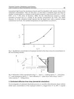
nonrelativistic particle in an infinitely high square well, etc.). In Figs. 2 and 3
we see typical energy distributions for the particular case of a constant density
of states. Of course, the q = 1 case reproduces the celebrated Boltzmann factor.
Notice the cut-off for q<1 and the long algebraic tail for q>1.
Since we have optimized the entropy, all the above considerations refer,
strictly speaking, to thermodynamic equilibrium. The word thermodynamic makes
allusion to “very large” (N →∞, where N is the number of microscopic par-
ticles of the physical system). The word equilibrium makes allusion to asymp-
totically large times (t →∞limit) (assuming a stationary state is eventually
achieved). The question arises: which of them first? Indeed, although both possi-
bilities clearly deserve the denomination ”thermodynamic equilibrium”, nonuni-
form convergences might be involved in such a way that lim

N→∞
lim
t→∞
could
differ from lim
t→∞
lim
N→∞
. To illustrate this situation, let us imagine a clas-
sical Hamiltonian system including two-body interactions decaying at long dis-
tances as 1/r
α
in a d-dimensional space, with α ≥ 0 (we also assume that the
potential presents no nonintegrable singularities, typically at the origin). If α>d
the interactions are essentially short- ranged, the two limits just mentioned are
basically interchangeable, and the prescriptions of standard statistical mechanics
and thermodynamics are valid, thus yielding finite values for all the physically
relevant quantities. In particular, the Boltzmann factor certainly describes real-
ity, as very well known. But, if 0 ≤ α ≤ d, nonextensivity is expected to emerge,
the order of the above limits becomes important because of nonuniform conver-
gence, and the situation is certainly expected to be more subtle. More precisely, a
crossover (between q = 1 and q = 1 behaviors) is expected to occur at t = τ (N).
If lim
N→∞
τ(N )=∞, then we would indeed have two (or even more) differ-
ent and equally legitimate states of thermodynamic equilibrium, instead of the
familiar unique state. The conjecture is illustrated in Fig. 4. We could of course
reserve the expression ”thermodynamical equilibrium” for the global extrema of
the appropriate thermodynamical energy. However, if the system is going to re-
main practically for ever in a local extremum, the distinction becomes physically

artificial.
Since we are discussing thermodynamical equilibrium, it is relevant to say a
few words on the present status of knowledge concerning the so-called 0
th
prin-
ciple of thermodynamics, or in other words, what happens with the transitivity
of thermodynamical equilibrium between systems if q = 1 ? This important
question is far from being transparent; it has already been addressed [82,83]
though, in our opinion, only preliminarily. However, after the instructive illus-
18 C. Tsallis
E / T’
01234
P(E,T’) / P(0,T’)
0.0
0.2
0.4
0.6
0.8
1.0
Fig. 2. Generalization (Eq. (48)) of the Boltzmann factor (recovered for q =1)as
function of the energy E at a given renormalized temperature T

, assuming a constant
density of states. From top to bottom at low energies: q =0, 1/4, 1/2, 2/3, 1, 3, ∞
(the vertical line at E/T

= 1 belongs to the limiting q = 0 distribution; the q →∞
distribution collapses on the ordinate). All q>1 curves have a (T

/E)

q/(q−1)
tail; all
q<1 curves have a cut-off at E/T

=1/(1 − q).
tration recently provided by Abe [84], a plausible scenario starts emerging. Let us
assume a composed isolated Hamiltonian system A + B (microcanonical ensem-
ble) such that (in some sense to be further qualified) we consider (i) H(A+B) ∼
H(A)+H(B), and (using quantum notation) (ii) ρ(A + B) ∼ ρ(A) ⊗ρ(B) (i.e.,
A and B are essentially independent in the sense of the theory of probabilities).
We shall also assume that (iii) A and B are in thermal equilibrium, i.e., their
energy distributions are essentially given by Eqs. (26) and (27). These three as-
sumptions seem at first sight incompatible, since the power-law of a sum does
not coincide with the product of the power-laws. In other words, the simultane-
Nonextensive Statistical Mechanics and Thermodynamics 19
E
0.1 1.0 10.0 100.0
P(E,T’) / P(0,T’)
0.0001
0.0010
0.0100
0.1000
1.0000
q=2
q=1
q=0.5
Fig. 3. Log-log plot of some cases like those of Fig. 2 (T

=1, 5 for each value of q).
ous demand of the three hypothesis seems to lead to only one type of statistics,

namely the q = 1 statistics. For this reason, it is stated in [82] that the present
generalized statistics is incompatible with the 0
th
principle, hence with ther-
modynamics. We believe this standpoint might be too narrow; it might well be
that q = 1 is sufficient but not necessary for the compatibility of the above three
hypothesis. Indeed, the thermodynamic limit (N →∞) might play a crucial role
in the problem, as elegantly illustrated on a simple example by Abe [84]! This
limit can be very subtle: for instance, several evidences are available [76,78,85]
which show that the N →∞and q → 1 can be not commutative. (Since at
t →∞for fixed N we expect q = 1, this non commutativity might be directly
related to the previously mentioned (N, t) → (∞, ∞) noncommutativity). Let
us now proceed with our argument. The three above assumptions imply that
U
q
(A + B) ∼ U
q
(A)+U
q
(B) (49)