a new type of structured artificial neural networks
Bạn đang xem bản rút gọn của tài liệu. Xem và tải ngay bản đầy đủ của tài liệu tại đây (147.38 KB, 7 trang )
A new type of Structured Artificial Neural Networks
based on the Matrix Model of Computation
Sergio Pissanetzky
Research Scientist. Memb er, IEEE. The Woodlands, Texas, United States
Abstract – The recently introduced Turing-complete
Matrix Model of Computation (MMC) is a con-
nectionist, massively parallel, formal mathematical
model that can be set up as a network of artificial
neurons and represent any other ANN. The model is
hierarchically structured and has a natural ontology
determined by the information stored in the model.
The MMC is naturally self-organizing and dynami-
cally stable. The Lyapunov energy function is inter-
preted as a measure of biological resources, the attrac-
tors correspond to the objects in the natural ontology.
The Scope Constriction Algorithm (SCA) minimizes
the energy by systematically switching the network
connections and reveals the ontology. In this paper
we consider the MMC as a modeling tool for applica-
tions in Neuroscience. We prove as a theorem that
MMC can represent ANNs. We present a new, more
efficient version of SCA, discuss the advantages of
MMC ANNs, and illustrate with a small example.
Keywords: neural networks, dynamic systems, ontologies,
self-organizing systems, artificial intelligence, semantic web.
1 Introduction and Previous
Work
The Matrix Model of Computation was introduced as
a natural algorithmic form of mathematical notation
amenable to be operated upon by algorithms expressed
in that same notation. It is formally defined as a pair of
sparse matrices, the rows of which are tuples in a rela-
tional database. Since MMC models can be easily cre-
ated by a parser from existing computer programs, and
then refactored by algorithm, the MMC was proposed as
a virtual machine for program evolution [1]. Subsequent
work [2] proved that any finitely realizable physical sys-
tem can be modeled by the MMC, and showed that the
model is naturally self-organizing by way of an algo-
rithm that organizes the information categorically into
weakly-coupled classes of strongly-cohesive objects, an
ontology [3]. Finally, applications to very diverse fields
such as theoretical Physics, business and UML models,
and OO analysis and design, were discussed and illus-
trated with small e xamples [4]. Relations have been
applied for the analysis of programs and a relational
model of computation has been proposed [5] and re-
cently characterized by investigating its connection with
the predicate transformer model [6].
In this paper we consider the MMC as a structured,
massively parallel, ge neralized, self-organizing, artificial
neural network. In Section 2 we define the MMC, in-
troduce terminology, discuss the hierarchical organiza-
tion and parallelism, examine combinations and con-
versions between artificial neurons or ANNs and MMC
models, training issues, and dynamics, and briefly com-
pare ANNs and MMC with humans. In Section 3 we
present prove that any ANN can be described as an
MMC model, and in Section 4 we present a new, more
efficient and biologically plausible version of the Scope
Constriction Algorithm, which gives the MMC its abil-
ity to self-organize. We close with a small example.
2 Overview of the Matrix Model
of Computation
2.1. Definition. The MMC is simple, yet very rich in
features. It is defined [1] as a pair of sparse matrices
[7] M = (C, Q), where C is the matrix of services and
Q is the matrix of sequences. The rows of C are the
services, and the columns of C are the variables used
by the services. A domain is the set of values allowed
for a variable, and there is a domain associated with
each variable. Each variable plays a certain role in the
service, indicated by A for an input variable or argu-
ment, C for an output variable or codomain, and M for
a modifiable variable or mutator. The roles A, C and
M are the elem ents of C in that service’s row.
The concept of service is very general. A service can
represent a neuron, a neural network, a primitive math-
ematical or logical operation in a standard computer, a
method in a class, or an entire MMC. Services can also
have their own memory visible only to the service (e.g.
a synaptic weight), and their own firing mechanisms.
Variables are also very general. A numerical variable
represents a value, a categorical variable represents an
instance of an object in a class. See Eq. (2) below for
a small example of a matrix C, or previous publications
[1, 2, 4] for more complete examples.
The rows of Q are the sequences. The columns of Q
include the actors that initiate sequences, the links be-
tween services, and the control variables that activate
or inhibit the links.
2.2. The data channel. The scope of a variable is the
vertical extent between the C or M where the variable
is first initialized and the terminal A where it is used
for the last time, in that variable’s column. The set
of scopes represents a data channel where data carried
by the variables flows from its source, the initializing
services, to its destinations, the services that use the
data. The sum of all scopes happens to be equal to the
vertical profile of C, immediately suggesting the use of
profile minimization techniques to make the data chan-
nel narrow, a highly desirable feature discussed below.
2.3. MMC algebra and transformations. MMC
has a rich algebra, which includes matrix operations
such as permutations, partitioning and submatricing,
relational operations such as joins, projections, normal-
ization and selection, and graph and set op e rations [1].
Algorithms can be designed based on these operations
to induce transformations on the MMC. Of particular
interest are refactorings, defined as invariant transfor-
mations that preserve the overall behavior of the model.
This is a general definition and it applies to all sys-
tems. The MMC has b ee n proposed for that purpose
[1]. Algorithms can also be designed for training or for
self-organization. One of them is discussed below.
2.4. Control flow graph, linear submatrices, and
canonical submatrices. A control flow gra ph (CFG)
is a directed graph G = (V, E) where a vertex v ∈ V
corresponds to each service in matrix C and an edge
e ∈ E corresponds to each tuple in matrix Q. A path
in the CFG represents a possible flow of control. The
path is said to be linear if its vertices have no addi-
tional incoming or outgoing edges except for the end
vertices, and the linear path is maximal if it can not be
enlarged without loosing the linear property. Given a
set of services S, a submatrix of services can be defined
by deleting from matrix C all rows with services not in
S and all columns with variables not used by the ser-
vices in S. A linear submatrix is a submatrix of services
based on the services contained in a linear path. Linear
submatrices are very common in a typical MMC model.
A service in a general MMC can initialize or modify
several variables at once, and a variable can be repeat-
edly re-initialized or modified. As a result, a submatrix
of services can contain many C’s and M ’s in each row or
column. However, the following simple refactoring can
convert any submatrix of services to a form without M’s
and exactly one C in every row and every column: (1) if
a service has n > 1 codomains C, expand it into n simi-
lar services that initialize one variable at a time, and (2)
if a variable is mutated or assigned to more than once,
introduce a new local variable for each assignment or
mutation. The resulting submatrix is square, and, since
there is only one C in every row and every column, a
suitable (always legal) column permutation can bring it
to a canonical form, where all the C’s are on the diag-
onal, the upper triangle is empty, the lower triangle is
sparse and contains only A’s, and the lowermost A in
each column is the terminal A in that column. Canoni-
cal submatrices correspond to the well-known single as-
signment representation, a connectionist model directly
translatable into circuits. Examples of canonical matri-
ces have been published ([4], figures 1, 2).
2.5. Ontologies. The roles A, C and M in a row of
matrix C es tablish an association between the service
in that row and the variables in the columns where the
roles are located. Since variables represent attributes
and can take values, and services represent the pro-
cesses and events where the variables participate, the
association represents an object in the ontological sense
[3]. We refer to this object as a primitive object, and
we say that matrix C defines a primitive ontology of
which the primitive objects are the elements and the
domains are the classes. Domains can be joined to form
super-domains, of which the original domains are the
subdomains. Sup e r-domains inherit the services and
attributes of their subdomains. Multiple-inheritance
is possible, and a subdomain can be shared by many
super-domains. In the ontology, the super-domains are
subclasses and the subdomains are super-classes, and
the super-classes subsume the subclasses. The sub-
domains of a super-domain can be replaced in matrix
C with a categorical variable representing that super-
domain, and similarly, the associated services can be
replaced with a “super-service” declared in an MMC
submodel in terms of the subservices, thus reducing the
dimension of C by submatricing. The process can be
continued on the simplified C, creating a hierarchy of
models and submodels that represents an inheritance hi-
erarchy. These features have been previously discussed
[1, 4]. Primitive objects do in fact combine sponta-
neously to form larger objec ts when the profile is mini-
mized, giving rise to the self-organizing property of the
MMC discussed below. In a biological system an ob-
ject could represent a cell, a neuron, a neural clique, an
organ, or an entire organism.
2.6. Parallelism. A service declaration is the root of
a tree, where only the external interface is declared in
a row of C but links present in matrix Q progressively
expand it in terms of more and more detailed declara-
tions, down to the deepest levels where declarations are
expressed in terms of services provided by the hardware
or wetware. To accommodate traditional computational
language, we say that services in a level invoke or call
those in the lower levels. The service declaration tree
also functions as a smooth serial/parallel interface as
well as a declarative/imperative interface. The services
near the top are sequentially linked by the scopes of the
variables, but as the tree expands, many new local vari-
ables are introduced and the interdependencies weaken,
allowing parallelism to occur. It is in this sense that
the MMC is considered as a massively parallel model.
The smooth transition between the two architectures is
a feature of MMC models.
2.7. ANN/MMC conversions and combinations.
Structured models entirely based on artificial neurons
can be formulated for any system by creating an initial
MMC model with serial services down to the level where
parallelism begins to appear, and continuing with tradi-
tional ANNs from there on. The services in the higher
levels are already connected in a network, and the in-
vo cations of the lower level services involve only eval-
uations of conditionals. Conditionals can, in turn, be
translated to ANN models, and at least one example of
such translations has been published [8]. In this way, a
homogeneous model consisting entirely of artificial neu-
rons is obtained, where collective be havior and robust-
ness are prevalent in the ANNs while a higher level of
functional and hierarchical organization is provided by
the underlying MMC. Another exciting p ossibility is to
combine the robustness and efficiency of ANNs with the
mathematical rigor and accuracy of traditional comput-
ers and the interoperability of the MMC by implement-
ing some services as ANNs and the rest as CPUs. The
theorem presented in the next Section clarifies some as-
pects of these conversions.
2.8. Training. MMC operations can be used to design
algorithms that add or organize MMC data. SCA is an
example. SCA does not add data but it creates new
information about data and organizes it into structure.
As such, it should be considered training. Direct train-
ing is another example. A modified parser can trans-
form a computer program into an MMC. Conversions
from other sources such as business models or theories
of Physics are possible [4]. There has been a recent
resurgence of interest in connectionist learning from ex-
isting information structures and processes [8, 9]. In
addition, the ANNs in the MMC support all traditional
modes of training. Conversely, a trained MMC network
will have a high ability to explain its decision-making
process, an important feature for safety-critical cases.
2.9. Self-organization. Under certain circumstances,
row and column permutations can be applied to C to
rearrange the order of the services and variables. The
permutations can be designed in such a way that they
constrict the data channel by reducing the scopes of
the variables, and at the same time cause similar prim-
itive objects to spontaneously come together and coa-
lesce into larger, more cohesive , and mutually uncou-
pled objects. This process is called scope constriction,
and is performed by the Scope Constriction Algorithm
discussed below. The transformation is also a refactor-
ing because it preserves the behavior of the m odel. The
process can continue with the larger objects, progres-
sively creating even larger objects out of the smaller
ones. The resulting hierarchical structure is the natural
ontology of the model. The natural ontology depends
on and is determined by the information contained in
the model, and is therefore a property of the model.
Definitions and properties of cohesion and coupling are
well established [10].
2.10. Dynamics. It is possible to imagine a scenario
where (1) new information keeps arriving, for example
from training or sensory perception, (2) the scope con-
striction process is ongoing, (3) the resulting natural
ontology evolves as a result of the changes in the body
of information, and (4) an ability to “reason” in terms
of the new objects rather than from the raw information
is developed. In such a scenario, some objects will stabi-
lize, others will change, and new objects will be created.
This scenario is strongly reminiscent of human learn-
ing, where we adapt our mental ontologies to what we
learn about the environment. It is also consistent with
recent work on neural cliques [11], suggesting that in-
ternal representations of external events in the brain do
not record exact details but are instead organized in a
categorical and hierarchical manner, with collective be-
havior prevalent inside each clique and a higher level of
organization and functionality at the network level. The
scenario can find other important applications, such as
semantic web development. Some of these ideas are
further discussed in Section 4. These ideas are not very
well supported by traditional ANNs. For quick refer-
ence, Table 1 shows some of the features of ANN and
MMC models that we have rated and compared with
humans. The comparison suggests that MMC models,
particularly MMC/ANN hybrids, may be better s uited
as models of the brain than ANNs alone, and may help
to develop verifiable hypotheses.
Table 1. Ratings of ANN and MMC features com-
pared with humans. 1 = poor, 2 = good, 3 = be st.
Supp orted feature humans ANN MMC
explanations 2 1 3
ontologies 3 1 3
expansion in size 3 1 3
expansion in detail 3 1 3
parallelism 3 3 3
sparse connectivity 3 2 3
self-organization 3 1 3
rigor and formality 2 1 3
3 Describing Artificial Neural
Networks with MMC models
The Theorem of Universality for the MMC states that
“Every finitely realizable physical system can be perfectly
represented by a Matrix Model of Computation” [2]. In
this Section we prove the following theorem:
Any ANN, consisting of interconnected artificial neu-
rons, can be equivalently described by an MMC model
where the neurons correspond to services and the con-
nections to scopes in the matrix of services.
This theorem follows from the theorem of universality.
However, in order to make the correspondence more ex-
plicit, we present the following proof by construction.
In the ANN model, a nonlinear neuron is describe d by
the following equation:
y
k
= ϕ
m
i=1
w
ki
x
ki
+ b
k
(1)
where k identifies the neuron, m is the number of inputs,
x
ki
are the input signals, w
ki
are the synaptic weights,
ϕ is the activation function, b
k
is the bias, and y
k
is the
output signal. Se rvice neuron k (nr k) in the following
MMC matrix of services C describes equation (1):
C =
serv ϕ {x
ki
} {w
ki
} b
k
y
k
{x
i
} − x
1
{w
i
} b
y
nr k A A A A C
nr A A A A C
(2)
where x
1
≡ y
k
, and set notation is used. Sets, func-
tions, etc, are considered objects in the ontological
sense, meaning for example that {x
ki
} stands not only
for the elements of the sets but also their respective car-
dinalities and other properties they may possess. Ser-
vice neuron (nr ) in eq. (2) represents a second
neuron that has the output signal y
k
from neuron k
connected as its first input x
1
. The scope of variable
y
k
, extending from the C to the A in that column, rep-
resents the network connection. The rest of the proof is
by recurrence. To add neurons, the same construction
is repeated as needed, and all connections to previous
neurons in the model are represented in the same way.
This completes the proof.
4 The Scope Constriction
Algorithm (SCA)
In this Section, we present a new version of the SCA
algorithm with a lower asymptotic complexity than the
original version [2]. The algorithm narrows the data
channel (§2.2) and reveals the natural ontology of the
model (§2.5) by minimizing the profile of the matrix
of services C. SCA operates on a canonical submatrix
(§2.4) of C, but for simplicity in presentation we shall
assume that the entire C is in canonical form. If N is
the order of C and j is any of its columns, then C
jj
= C.
If there are any A’s in that column, then the downmost
A, say in row D
j
, is the terminal A, and the length of
the scope of the corresponding variable is D
j
− j. If
there are no A’s, the variable is an output variable and
D
j
= j. The vertical profile of C is:
p(C) =
N
j=1
(D
j
− j). (3)
The variable in column j is initialized by the C in that
column. Then, the data travels down the scope to the
various A’s in column j, and then horizontally from the
A’s to the C’s in the corresponding rows, reaching as
far as the C in column D
j
, which corresponds to the
terminal A in column j. Ne w variables are initialized
at the C’s, and the process repeats itself. The “conduits
of information” that carry the traveling data constitute
the data channel, and the lengths of the scopes are a
measure of its width. The maximum width W
m
(C) and
the average width W
a
(C) of the data channel are defined
as follows:
W
m
(C) = max
j
(D
j
− j) (4)
W
a
(C) = p(C)/N (5)
SCA’s goal is to reduce the lengths of the scopes and
the width of the data channel by minimizing p(C).
In the canonical C, services are ordered the same
as the rows. Matrix Q still applies, but is irrelevant
because it simply links each service unconditionally to
the service below it. Commuting two adjacent services
means reversing their order without affecting the overall
behavior of the model. The lengths of the scope s and
the value of the profile p(C) depend on the order of the
services, hence SCA achieves its goal by systematically
seeking commutations that reduce the profile. Since a
behavior-preserving transformation is a refactoring, a
commutation is an element of refactoring and SCA is a
refactoring algorithm.
Commutation is legal if and only if it does not reverse
the order of initialization and use of any variable. More
specifically, a service in row i initializes the variable in
column i, because C
ii
= C. Since this is the only C
in that row, the service in row i and the service in row
i + 1 are commutative if and only if C
i+1,i
is blank. In
other words, commutations are legal provided the C’s
stay at the top of their respective columns. For exam-
ple, the two services in eq. (2) are not commutative
because of the presence of the A under the C in column
y
k
. Commutation preserves the canonical form of C.
Repeated commutation is possible. If service S in
row i commutes with the service in row i − 1, the com-
mutation can be effected, causing S to move one row up,
and the service originally in row i − 1, one row down.
If S, now in row i − 1, commutes with the service in
row i − 2, that commutation can be effected as well,
and so on. How high can S go? Since there are no A’s
above the C in column i of S, all commutations will
be legal until the rightmost A in row i, say in column
R
i
, gets to row R
i
+ 1 and encounters the C in row
R
i
of that column. Thus, service S can go upwards as
far as row R
i
+ 1 by repeated commutation. Similarly,
service S in row i can commute with the service in row
i +1, then with the service in row i + 2, and so on, until
the C in column i of S encounters the uppermost A in
that column, say in row U
i
, namely all the way down to
row U
i
− 1. The range (R
i
+ 1, U
i
− 1) is the range of
commutation for service S in row i.
Repeated commutation of services amounts to a per-
mutation of the rows of C. To preserve the canonical
form, a symmetric permutation of the columns must
follow. Thus:
C ← P
T
CP. (6)
where P is a permutation matrix. T he symmetric per-
mutation is also behavior-preserving, and it is a refac-
toring. SCA can be formally described as a procedure
that finds P such that p(C) is minimized. The mini-
mization of p(C) is achieved by systematically examin-
ing sets of legal permutations and selecting those that
reduce p(C) the most. However, SCA does not guar-
antee a true minimum. In the process, p(C) decreases
smoothly, but individual scopes behave in a complicated
way as they get progressively constricted against the
constraints imposed by the rules of commutation. The
refactoring forces related services and variables to co-
alesce into highly cohesive, weakly coupled clusters, a
phenomenon known as encapsulation. The clusters are
recognized because few or no scopes c ross intercluster
boundaries, they correspond to objects, and the term
constriction is intended to convey all these ideas. The
original ve rsion of the algorithm, known as SCA2, op-
erates as follows:
(1) Select a row i of C in an arbitrary order.
(2) Determine the range of commutation R
i
, U
i
for the
service in that row.
(3) For each k, R
i
< k < U
i
, calculate p(C
k
), where C
k
is obtained from C by permuting the service from
row i to row k, and select any k that minimizes p.
(4) Permute the service to the selected row.
(5) Rep eat (1-4) until all rows are exhausted.
(6) Rep eat the entire procedure until no more reduc-
tions are obtained.
To calculate the asymptotic complexity of SCA2 we as-
sume that C, being sparse, has a small, fixed number of
off-diagonal nonzeros per row. Assuming the roles are
indexed by service, the calculation of R
i
, U
i
requires a
small, fixed number of operations per row, or O(N) op-
erations for step (2) in total. The calculation of the
profile, eq. 3, requires the calculation of D
j
for each
column j, which takes a small, fixed numb er of oper-
ations per column, or O(N) in total. In a worst case
scenario, the range for k in step (3) may be O(N), so
step (3) will require O(N
2
) operations per row, or a
total of O(N
3
) for the entire pro c edure. The rest of
the operations is O(N ) or less. Thus, the asymptotic
complexity of SCA2 is O(N
3
), caused by the repeated
calculation of the profile. The new version of SCA dif-
fers from SCA2 only in step (3), as follows:
(3) (new version). Calculate ∆
i,k
(C) for each k, R
i
<
k < U
i
, and select the smallest.
∆
i,k
(C) is the increment in the value of the profile when
the service in row i is reassigned to row k, and can be
calculated based on the expression:
∆
i,i+1
(C) = q
i
+ p
i
− q
i+1
. (7)
Let n
i
be the number of terminal A’s in row i, m
j
be the number of terminal A’s in column j (0 or 1),
and q
i
= n
i
− m
i
be the excess of terminal A’s for
row/column i. Also let p
i
be the number of terminal
pairs in row i. We say that a terminal pair exists in
row i, column j when C
i,j
= A and C
i+1,j
is a terminal
A. Equation 7 follows, and ∆
i,k
is obtained by rep eate d
application of that equation.
Assuming as we did before that the roles are indexed
by service, and the services by row and column, the cal-
culation of R
i
, U
i
, q
i
, p
i
and ∆
i,i+1
each takes a small,
fixed number of op erations, and the calculation of ∆
i,k
for all k takes O(N) operations. Thus, the new step (3)
takes O(N) operations, and the asymptotic complex-
ity of SCA is O(N
2
). The improvem ent in complexity
is due to the fact that actual values of the profile are
never calculated. The new SCA is a second order al-
gorithm because the neutral subsets are properly taken
care of as part of the range of commutation [2].
SCA is a natural MMC algorithm in the sense that it
modifies the MMC itself and is universal. As such, and
since the MMC is a program [1], SCA can be installed
as a part of MMC itself, making the MMC a dynamical
system, a self-refactoring MMC where the energy (Lya-
punov) function is the profile p(C) and the attractors
are the objects that SCA converges to. Since SCA is
behavior-preserving, it can run in the background with-
out affecting the operation of the MMC. The dynamical
operation is characterized by two well-differentiated but
coexisting processes: (1) new information arrives as the
result of some foreground training process and is ap-
pended to C, resulting in a large profile, and (2) SCA
minimizes the profile and updates the natural ontology
by creating new objects or modifying the existing ones
in accordance with the information that arrives. The
objects are instated as new categorical variables and op-
eration continues, now in terms of the new objects. Such
a system allows higher cognition such as abstraction and
generalization capabilities, and is strongly reminiscent
of the human mind, particularly if the creation of ob-
jects representing the natural ontology is inte rpreted as
“understanding”, and the recognition of objects for fur-
ther processing as “reasoning”. These views offer a new
interpretation of learning and meaning.
The term “energy” used above refers to resources
in general, including not just physical energy but also
building materials, or some measure of the physical re-
sources needed to implement the system. When neurons
form their axons and dendrites they must maximize in-
formation storage but minimize resource allocation [12].
The correspondence between the scopes and the net-
work connections discussed in Sec tion 3 suggests a cor-
respondence between their respective lengths as well, in
which case there should be a biological SCA-type pro-
cess that rewires the network by proximity or migrates
the neurons to shorten their connections. Either way,
the net result is that neurons close in the logical se-
quence become also geometrically close, creating an as-
sociation between function and information similar to
an OOP object. These obse rvations are consistent with
the minimum wiring hypothesis, as well as with Horace
Barlow’s efficient coding hypothesis, Drescher’s schemas
[13], and Gell-Mann’s schemata [14]. Similar observa-
tions may apply to other biological structures such as
organs, or to entire organisms.
In comparison with other algorithms such as MDA,
we note that SCA uses no arbitrary parameters, is ex-
pandable in the sense that new elements and new classes
can be added and the model can grow virtually indef-
initely, both in size and refinement, and is biologically
plausible because it uses local properties, likely to be
available in a cell or an organ. MDA, instead, uses
mathematical equations, very unlikely to exist in a bio-
logical environment.
5 An SCA example
Applications for SCA can be found in many domains.
An example in theoretical Physics was published [4],
where the model consists of 18 simple equations with
30 variables, and SCA constructs an ontology consisting
of a 3-level multiple-inherited hierarchy with 3 objects
in the most specialized class, that describes an impor-
tant law of Physics. Here we consider classification.
For classification, associations must be established be-
tween some property of the objects to be classified and
a suitable discriminant or classifier. Then, SCA finds
patterns and classifies the objects dynamically. For
example, if the objects are points in some space, then
the discriminant is a mesh of cells of the appropriate
dimensionality and desired resolution, points are associ-
ated with the ce lls that contain them, and the resulting
classes are clusters of points. If the objects are neurons
that fire at different times, the discriminant is a mesh
of time intervals, neurons are associated with the time
intervals where they fire, and the classes would be neu-
ral cliques [11]. Table 2 summarizes these observations.
Table 2. Parameters used for SCA classification.
objects property discriminant class
points position mesh of cells cluster of points
neurons firing event time mesh neural clique
Our classification example involves a set of 167 points
defined by their coordinates in som e space. In the ex-
ample, the space is two-dimensional, but the number of
dimensions is irrelevant. In Figure 1, the points are at
the center of the symbols. The discriminant consists of
4 overlapping meshes, simulating the continuity of the
space. The basic mesh consists of cells of size 1 × 1,
and 3 more meshes are superposed w ith relative shifts
of (0.5, 0), (0, 0.5), and (0.5, 0.5), respectively. The
resulting matrix of services C is of order 1433, and is
already in canonical form.
× ×
××
×
×
×× × ×
×
×
×
×
×
×
×
×
×
×
×
×
×
×
×
×
×
×
×
+ +
+
+ +
+
+
+
+ +
+
+
+
+
+ +
+
+ + + + +
+ +
+
+
+
+
+ + + + + +
+
+
+
+
+
+ +
+ +
+
+ +
+
+
+
+
+ +
+
+
+ +
+
+
+
+
+ +
+ +
+
+
+
+ + +
+
+ +
+
+ +
+
+
+
+ + +
+
+ +
+
+
++
+ + +
+ +
+ + +
+
+ + +
++
+
△
△
△
△ △
△
△
△
△
△
△
△
△
△
△
△
△
△
△ △ △
△
△
△ △
△△ △
△
△
△ △△ △
Figure 1. The set of points for the example. The given
points are at the center of the symbols, the symbols in-
dicate the resulting classes.
The initial 167 services initialize the points (assuming
each service knows where to initialize them from, which
is irrelevant for our purpose). The next 345 services
initialize all the necessary cells. The last 921 services
establish the point/cell associations. Each service takes
one point and one cell as arguments (indicated with an
“A” in that row and the corresponding columns), and
initializes one association (a “C” in that association’s
column). The initial profile is 299,565 and the data
channel’s average width is 209.1 and maximum width
is 1266. SCA converges in two passes, leaving a final
profile of 15,642 and a data channel with an average
width of only 10.9 and a maximum width of 705. The
points are classified into three clusters as indicated by
the symbols in Figure 1. The ontology for this system
consists of just one class with three objects, the clusters.
6 Conclusions and outlook
MMC is a form of mathematical notation designed to
express our knowledge about a domain. Any ANN can
be represented as an MMC, and ANN/MMC combina-
tions are also possible. The models are formal, have a
hierarchical but flexible organization, and are machine-
interpretable. Algorithms can be designed to induce
transformations, supported by a rich algebra of opera-
tions. All modes of training are inherited. In addition,
ANN/MMC models can be directly constructed from
existing ontologies such as business mo dels, computer
programs or scientific theories.
We believe that the MMC offers an excellent oppor-
tunity for creating realistic models of the brain and
nervous system, particularly when used in combination
with traditional ANNs. A model can consist of many
submodels representing different subsystems and hav-
ing different degrees of detail, depending on the extent
of the knowledge that is available or of interest for each
subsystem. It is possible to start small and then grow
virtually indefinitely, or to add fine detail to a particular
submodel of interest, while still retaining interoperabil-
ity. Dynamic, self-organizing submodels will find their
own natural ontologies, which can then be compared
with observation, an approach that is radically different
from the more traditional static man-made ontologies,
and has remarkable similarities with human and animal
learning. MMC offers a framework for constructing,
combining, sharing, transforming and verifying ontolo-
gies.
We conclude that the MMC can serve as an effec-
tive tool for neural modeling. But above all, the MMC
will serve as a unifying notion for complex systems, by
bringing unity to disconnected fields, organizing infor-
mation, and providing convergence of concepts and in-
teroperability to tools and algorithms.
References
[1] Sergio Pissanetzky. “A relational virtual machine
for program evolution”. Proc. 2007 Int. Conf. on
Software Engineering Research and Practice, Las Vegas,
NV, USA, pp. 144-150, June 2007. In this publication,
the Matrix Model of Computation was introduced with
the name Relational Mo del of Computation, but was
later renamed because of a name conflict.
[2] Sergio Pissanetzky. “The Matrix Model of Compu-
tation.” Proc. 12th World Multi-Conference on Sys-
temics, Cybernetics and Informatics: WMSCI ’08. Or-
lando, Florida, USA, June 29 - July 2, 2008.
[3] B. Chandrasekaran, J. R. Josephson, and V. R. Ben-
jamins. “What are ontologies, and why do we need
them? ” IEEE Intelligent Systems, Vol. 14(1), pp. 20-
26 (1999).
[4] Sergio Pissanetzky. “Applications of the Matrix
Model of Computation.” Proc. 12th World Multi-
Conference on Systemics, Cybernetics and Informatics:
WMSCI ’08. Orlando, Florida, USA, June 29 - July 2,
2008.
[5] Jifeng He, C. A. R. Hoare, and Jeff W. Sanders.
“Data refinement refined.” Lecture Notes In Computer
Science, Vol 213, pp. 187-196 (1986).
[6] Jeff W. Sanders. ”Computations and Relational
Bundles.” Lecture Notes in Computer Science, Vol 4136,
pp. 30-62 (2006).
[7] Sergio Pissanetzky. Sparse Matrix Technology. Aca-
demic Press, London, 1984. Russian translation: MIR,
Moscow, 1988.
[8] J. P. Neto. “A Virtual Machine for Neural Com-
puters.” S. Kollias et al. (Eds). ICANN 2006, Part I,
LNCS 4131, pp. 525-534, 2006.
[9] W. Uwents, G. Monfardini, H. Blockeel, F. Scarcelli,
and Marco Gori. “Two connectionist models for graph
processing: an experimental comparison on relational
data.” Mining and Learning with Graphs Workshop
(MLG 2006), ECML/PKDD, Berlin (2006).
[10] S. R. Chidamber and C. F. Kemerer. “A metrics
suite for object oriented design.” IEEE Trans. on Soft-
ware Engng., Vol. 22, pp.476-493 (1994).
[11] L. Lin, R. Osan, and J. Z. Tsien. “Organizing prin-
ciples of real-time memory encoding: ne ural clique as-
semblies and universal neural codes.” Trends in Neuro-
sciences, Vol. 29, No. 1, pp. 48-57 (2006).
[12] D. B. Chklovskii, B. W. Mel, and K. Svoboda.
“Cortical rewiring and information storage.” Nature,
Vol 431, pp. 782-788 (2004).
[13] G. Drescher. Made-up Minds. MIT Press, Cam-
bridge, MA (1991).
[14] M. Gell-Mann. The Quark and the Jaguar. W. H.
Fre eman and Co, New York (1994).
Acknowledgements. To Dr. Peter Thieb erger (BNL,
NY) for his generous and unrelenting support, without
which this might not have happened.