Section 6 1 TRƯỜNG ĐIỆN TỪ
Bạn đang xem bản rút gọn của tài liệu. Xem và tải ngay bản đầy đủ của tài liệu tại đây (154.44 KB, 22 trang )
Slide Presentations for ECE 329,
Introduction to Electromagnetic Fields,
to supplement “Elements of Engineering
Electromagnetics, Sixth Edition”
by
Nannapaneni Narayana Rao
Edward C. Jordan Professor of Electrical and Computer Engineering
University of Illinois at Urbana-Champaign, Urbana, Illinois, USA
Distinguished Amrita Professor of Engineering
Amrita Vishwa Vidyapeetham, Coimbatore, Tamil Nadu, India
6.1
Transmission Line
6.1-3
Parallel-Plate Line
d
Vg t
y
+
-
x
z
Neglect fringing (d << w).
w
6.1-4
E Ex z , t ax ; H H y z , t ay
z
+
x
H
-
+
+
, ,
-
+
-
+
E, Jc
-
d
6.1-5
d
V z , t Ex z, t dx
x 0
d Ex z , t
V z, t
Ex z , t
d
I z , t w J s z , t
w H y z , t
I z, t
H y z, t
w
6.1-6
H y
Ex
z
t
H y
Ex
Ex
z
t
V
z d
I
t w
I
V
z w
d
V
t d
6.1-7
V
d I
z
w t
Consider the circuit
I z, t
I
w
V
z
d
w V
d
t
I z z, t
L z
+
V z, t
z
-
+
G z
z
C z
V z z, t
z z
6.1-8
Then
V
I
L
z
t
I
V
GV C
z
t
Transmission
Line
Equations
d
L=
, inductance per unit length
w
w
G=
, conductance per unit length
d
C = w , capacitance per unit length
d
6.1-9
Transverse Electromagnetic (TEM) Waves
a
Ez Hz 0
b
V z , t E z , t d l
a
I z , t H z , t d l
C
C
x
b
z
y
6.1-10
Distributed Equivalent Circuit
L z
G z
L z
C z
G z
C z
z
Assumes perfect conductors but lossy dielectric.
6.1-11
Transmission-Line Equations
V
I
L
z
t
I
V
GV C
z
t
L = Inductance per unit length (H/m)
C = Capacitance per unit length (F/m)
G = Conductance per unit length (S/m)
6.1-12
In general, conductors are also lossy. Then, the waves
are not exactly TEM waves.
V
I
RI L
z
t
I
V
GV C
z
t
R = Resistance per unit length (/m)
6.1-13
Lossless Line
(Perfect Conductors, Perfect Dielectric)
V
I
L
z
t
I
V
C
z
t
Combining, we obtain
2V
2V
LC 2
2
z
t
Wave
Equation
6.1-14
Solution:
V z , t Af t z vp Bg t z vp
wave
wave
1
1
vp
LC
velocity of propagation
Note, LC =
6.1-15
V
I
From
L ,
z
t
I
1 V
t
L z
1
Af t z vp Bg t z vp
Lvp
1
I z , t Af t z vp Bg t z vp
Z0
L
where Z0
characteristic impedance of the line
C
6.1-16
Thus
V V
t z v V t z v
p
p
V t z vp V t z vp
I
Z0
Z0
wave wave
1
vp
LC
L
Z0
C
6.1-17
Parallel-Plate Line
d
L
w
C w
d
d
Z0
w
w
d
d << w
6.1-18
Coaxial Cable
L 1n b
2
a
2
C
b
1n
a
Z0 1n b
2
a
b
a
6.1-19
Parallel-Wire Line
L cosh 1 d
a
C
cosh 1 d
a
Z0 cosh 1 d
a
a
a
2d
6.1-20
Parallel-Strip Line (d/w 1)
imbedded in a homogeneous medium
w
2d
Z0
1n 8d w
w 4d