Theories of Gold Price Movements: Common Wisdom or Myths
Bạn đang xem bản rút gọn của tài liệu. Xem và tải ngay bản đầy đủ của tài liệu tại đây (789.94 KB, 27 trang )
Undergraduate Economic Review
Volume 6
|
Issue 1 Article 5
2010
eories of Gold Price Movements: Common
Wisdom or Myths?
Fan Fei
University of Michigan - Ann Arbor,
Kelechi Adibe
University of Michigan Law School,
is Article is brought to you for free and open access by the Economics Department at Digital Commons @ IWU. It has been accepted for inclusion in
Undergraduate Economic Review by an authorized administrator of Digital Commons @ IWU. For more information, please contact
©Copyright is owned by the author of this document.
Recommended Citation
Fei, Fan and Adibe, Kelechi (2010) "eories of Gold Price Movements: Common Wisdom or Myths?," Undergraduate Economic
Review: Vol. 6: Iss. 1, Article 5.
Available at: hp://digitalcommons.iwu.edu/uer/vol6/iss1/5
1. Introduction
Gold has a unique status in the economic world: a precious medal with wide
uses, a store of wealth, and for a long time, the measure of economic power of
nations and the cornerstone of international monetary regimes. In recent years, the
world witnessed an aggressive growth in gold price. The role of gold in
investment has drawn more attention since this transformational economic crisis
began to unfold in 2008. This paper is another attempt to disentangle the price
movement of gold after the Bretton-Woods system, the last international
monetary regime based on gold. To what extents can we understand the price
movement of gold? Can we find support for some popular opinions about gold on
finance media? For instance: is gold a safe haven, a negative-beta asset, or an
inflation hedge? How should we think about gold: a commodity or a currency?
This paper provides some thoughts on these questions.
1.1 Gold and the Gold Standard
Returning to gold standard has never been seriously discussed for decades.
After waves of gold reserves sales in the last fifteen years or so, gold is being
seen more and more as a common commodity. But history has a long shade in
economic thinking and economic activities; one cannot fully understand the
current status of gold and its price fluctuations while totally disregarding its
history.
Gold has been used in rituals, decorations, and jewelry for thousands of years.
Its unusual chemical properties—high density, superb malleability, imperishable
shine—and its genuine rarity all contribute to it being the most coveted
commodity in nearly every culture. But it is not until in the late nineteenth century
when the gold standard formed that gold went onto the central stage of global
economic life. In that half a century, on one hand there was a huge supply shock
of gold as a result of the Gold Rushes; on the other hand there was soaring
demand for a global monetary medium of high value to finance the rapid
industrialization and the emerging international trade and banking. And the fact
that Britain, the indisputable super power then, had adopted the gold standard and
a series of historical incidents led all major economies save China signed up to
gold by 1900.
The gold standard, under which gold coins and fiat money could be converted
at banks freely at a pre-set official rate and nations settled balance differences in
gold, has intrinsic deflationary pressure: the inelastic supply of gold always made
the money supply insufficient in a growing economy with rising productivity
(insufficient liquidity). To keep up with demand for money, monetary authorities
developed the “gold-exchange standard”: bank notes of major economies could
also be treated as reserve assets. But the faith in the convertibility of foreign
reserves (ultimately the commitment of monetary policy of reserve-currency
1
Fei and Adibe: Gold Price Theories: Common Wisdom or Myths?
Produced by The Berkeley Electronic Press, 2010
countries) was always fragile. The huge global deflation after the collapse of
foreign reserves under the interwar gold-exchange standard and the “neighbor thy
beggar” policies largely caused the Great Depression.
After the Great Depression and WWII, a new international monetary system,
the Bretton-Woods system was founded. The implemented Bretton-Woods
system
1
was a fix-exchange-rate gold-dollar standard regime. Under it, the U.S.
monetary authority was immediately put into a dilemma: with the U.S. being the
sole de-facto reserve-currency country, whichever policy the Fed
implemented—expansionary or tight money, it would lead to either the erosion of
confidence on the dollar or a deflationary pressure worldwide. Also, domestic
policy goals, such as maintaining economic growth and low employment, and the
responsibility of reserve-currency country to stabilize the value of the dollar were
often conflicting. These problems worsened in 1960s with the increasing
expenditure on social welfare programs and the war in Vietnam. Pressure from
foreign governments and speculators on financial markets and U.S. government
pushed Bretton-Woods System to an end in 1973.
Since 1973, gold could be publicly traded with little government
intervention.
2
It is no longer directly linked to any nation’s monetary policy or
the value to any currency. The central banks continued to hold considerable
amount of gold reserves for strategic or confidence reasons. There have been
debates in academia on the better use of the former monetary gold.
3
Since 1990s,
Bank of England, Swiss National Bank and central banks of Eastern Bloc
countries have sold great amount of their gold reserves.
1.2 Gold Demand
Gold has both private demands and government demands. As previously
discussed, in the gold-standard era, government demand is monetary gold. In post
Bretton-Woods era, central banks still hold great amount of gold reserves as
strategic assets (“war chest”) but the government demands are not that active and
influential as they were in gold-standard years.
4
Private demands can be further
1
The implemented Bretton-Woods system is pretty different from the designs. See the book “A
Retrospective on the Bretton Woods System” for reference.
2
This is only the case in the West. In all Communist countries, private possession and trading of
gold bars or coins were prohibited. These policies ended in the Eastern Bloc countries and the
former Soviet Union countries in early 1990s. But in countries like China or North Korea, the state
still holds tight control over gold production and private possession of gold.
3
For instance, see the paper “The benefits of expediting government gold sales” by Henderson
and Salant et al.
4
Most governments don’t increase their holds for gold. Many countries began to their gold
reserves. On the whole, government demands have been negative (in other words, net supply) for
at least a decade. Only few countries, like Russia and China, are increasing their gold reserves in
recent years.
2
Undergraduate Economic Review, Vol. 6 [2010], Iss. 1, Art. 5
/>
divided using different criteria. One division is investment (ETFs, bullions, bars
etc.) and non-investment (jewelry, industrial and dental) demands. Another
division is depletive uses (manufacturing and dentistry) and non-depletive uses
(bullions, jewelry, ornamentation and hoarding etc.).
What are the shares of different gold demands? We couldn’t find any data for
the gold-standard era. But there have been estimates that between half and
two-thirds of the annual production went to private uses.
5
One snapshot of recent
years’ gold demand breakup came from 2007.
6
In that year, the gold reserves of
central banks and international institutions (IMF, for instance, is a large holder of
gold reserves) decreased by 504.8 tons, which meant a negative demand or a net
supply. All newly mined gold went to private sector: More than two thirds of it
(2398.7 out of 3558.3 tons) went to jewelry, the industrial and dental demands
used up approximately 13% of the production. The remaining fed private
investment needs. Geographically, India consumed 773.6 tons of gold, about 20%
of the world’s production; greater China region consumed 363.3 tons, ranking the
second. In terms of “stock”, a rough estimate is that the total above-ground stocks
of gold are about 161,000 tons
7
now, 51% of which are in terms of jewelry.
Official sectors hold nearly 30000 tons (18%), (private) investment 16%, and
industrial 12%.
1.3 Gold Supply
Gold supply comes from mining, sales of gold reserves, and “old gold scrap”
(the recycling of gold). The gold mining went hand in hand with the geographical
discovery of the earth by mankind. During the Gold Rushes years (from 1850 to
1900), about twice as much gold was mined as in previous history. The annual
production of gold continued to increase dramatically in the twentieth century:
from less than 500 tons per year in the 1900s all the way to more than 2000 tons
per year in late 1980s. In the last fifteen years though, the annual mining
production fluctuated around 2500 tons,
8
which revealed the increasing difficulty
of finding new deposits and mining and extraction in non-rich sites. Most of the
gold left to be mined exists as traces buried in marginal areas of the globe, for
instance, in the rain forests of Indonesia, the Andes and on the Tibetan plateau of
China. Gold mining has been bringing environmental disasters in forms of
mercury linkage, deforestation and waste rocks among others to Africa, Latin
America and East and Southeast Asia. This has drawn more and more attention
5
The discussion is in Barsky and Summers (1988).
6
The 2007 demand data is from World Gold Council website.
7
Whether this figure means the amount of gold have been mined in all human history or only
those that are available to this generation is unclear.
8
The sources of data for the gold worksheet are the mineral statistics publications of the U.S.
Bureau of Mines (USBM) and the U.S.Geological Survey (USGS)—Minerals Yearbook (MYB).
3
Fei and Adibe: Gold Price Theories: Common Wisdom or Myths?
Produced by The Berkeley Electronic Press, 2010
worldwide.
1.4 Gold Price Movements
We chose the perspective of testing some commonly-held or heatedly-debated
opinions about the price of gold as a means to analyze its price movement.
Several common-wisdom “theories” are considered:
Firstly, people claim that as gold remains the eternal symbol of wealth in
people’s minds; people will switch their investments to gold in ages of turbulence.
Gold is the “safe haven” on the financial market. To test this hypothesis, we look
into various “fear” measures: volatility in the stock market, consumer
expectations of the future, and bond risk premiums (the difference in yield
between Aaa and Baa bonds) and check the correlations of those and gold price
movements. A somewhat related hypothesis—the negative-beta asset hypothesis
(“gold goes up when everything else going down”) is also tested.
Secondly, people marketing gold investment products will always describe
gold as an “inflation hedge”. A straightforward analysis is provided on the real
gold price (level), the return of gold and expected and actual inflation to test this
claim.
Instead of viewing gold as a special asset, we suggest the data suggest it is
more reasonable that we view gold as another currency, whose value is a
reflection of the value of U.S. dollar. We investigate extensively on the
relationship between gold price and dollar and dollar-valued assets in section 5.
Some other less theoretical sayings are considered too, for example the effect
of surging demands in India and China and the central bank gold reserve sales on
the gold price.
The remainder of the paper is organized as follows. Section 2 describes the
data used in this study. The next three parts discuss three hypotheses one by one:
section 3 focuses on safe haven hypothesis and whether gold behaves as a
negative beta asset, section 4 is on inflation hedge hypothesis, and section 5
investigates the relationship between gold price and U.S. dollar. Section 6 reports
results from multiple linear regressions. A semi-structural VAR model is
constructed and analyzed in section 7 before we conclude.
2. Data
Our data includes real gold price, various “fear” indicators, U.S. inflation rate,
real long-term interest rate, indicators of real economic activity and the exchange
rate. For gold price, we used the closing price on the last trading day for gold each
month on the New York Mercantile Exchange. The data series ranges from
January 1956 to October 2008 and is available on the Commodity Research Board
(CRB) website. The figures are in 2008 dollars. Overall, gold prices appear to
have been in a downward trend since the peak in the early 1980s but showed an
4
Undergraduate Economic Review, Vol. 6 [2010], Iss. 1, Art. 5
/>
impressive upward movement in recent five to ten years, as shown in Figure 1. A
simple serial correlation test showed the monthly gold price is highly serial
correlated. Figure 2 shows the trend of monthly gold returns, or month-to-month
gold price changes, in percentage. It is not serially correlated but quite noisy.
0
400
800
1200
1600
2000
1980 1985 1990 1995 2000 2005
Figure 1: Real Gold Price 1978-2008
-500
-400
-300
-200
-100
0
100
200
300
400
1980 1985 1990 1995 2000 2005
Figure 2: Monthly Gold Returns 1978-2008
5
Fei and Adibe: Gold Price Theories: Common Wisdom or Myths?
Produced by The Berkeley Electronic Press, 2010
We considered three “fear” indicators for this study. The first one is the stock
market volatility; in this case the squared monthly returns of the S&P 500 Index
suggested by Cutler, Poterba and Summers (1988). The second is the University
of Michigan Index of Consumer Expectations, which represents sentiment of the
general public about
the economy in the near future. Higher scores represent
optimism and lower scores represent pessimism.
9
The index is by construction
stable. The last one is a bond premium: the difference in yields between Moody
rated Aaa and Baa seasoned corporate bond. This widening of the premium is an
indicator of growing uneasiness on the market.
The actual inflation measure is just the monthly change of the Consumer
Price Index (urban, all goods). The expected inflation measure comes from the
University of Michigan/Reuters Survey of Consumers, in which they reported the
median price change the consumers expected over the next twelve months.
We have two measures regarding the value of dollar. The first one is the
exchange rate, to be specific, the Trade Weighted Exchange Index provided by St.
Louis Fed. The index is de facto the exchange rate of U.S. dollar against a basket
of currencies, which includes currencies from the Euro Area, Canada, Japan,
United Kingdom, Switzerland, Australia, and Sweden. High values for the index
mean a relatively strong dollar, and low values for the index mean a weak dollar.
The second one is the value of dollar-backed assets, in this case the real ten-year
Treasury bond rate.
We consider three macroeconomic activity measures: monthly return of the
S&P 500 Index, U.S. industrial production (detrended) and the cargo freight rate
index used in Kilian (2007).
Our sample period is from January 1978 to December 2007. We used
monthly data.
10
3. Safe Haven Hypothesis and Gold as a Negative-Beta Asset
People often associate gold with the notion of a safe haven. We define safe
haven assets to be assets that people would like to invest in when uncertainty and
fear increases. These assets would preserve their values in times of turmoil or
recession. So we investigate the overall relationship between return on gold and
various fear measures mentioned above to testify this hypothesis. If this
9
This index is based on the relative scores (the percent giving favorable replies minus the percent
giving unfavorable replies plus 100) of each of the five survey questions. Higher scores represent
optimism and lower scores represent pessimism. The indices are monthly published by Reuters
and Survey Research Center of University of Michigan.
10
The monthly available series include: US Industrial Production Index, U.S. CPI, Kilian Dry
Cargo Freight Rate Index and University of Michigan Consumer Expectation Index. The Moody’s
BAA and AAA seasoned corporate bond yields, Trade Weighted Exchange Index: Major
Currencies, 10-year Treasury bond rate are averages of daily data.
6
Undergraduate Economic Review, Vol. 6 [2010], Iss. 1, Art. 5
/>
hypothesis is true, if people become more fearful in the markets, the price of gold
should rise. The safe haven hypothesis is closely related to the negative-beta-asset
hypothesis. We define negative-beta assets to be those whose returns are
negatively correlated with macroeconomic performance, measured by monthly
return of S&P 500, the dry cargo freight rate index introduced in Kilian (2007)
and the U.S. industrial production in our study. First, we look at the “fear
premium” side to the safe haven hypothesis.
3.1 Gold and Volatility
We started looking at the effect of volatility on the price of gold to test the
safe haven hypothesis. Looking at Figure 3, a graph of the logged real price of
gold and the constructed volatilty measure, the safe haven effect is not evident.
Many of the most salient moves in the graph either provide evidence that is
contrary to the idea of gold being a safe haven, or provide no evidence at all.
From 1978 to 1980, the price of gold rises from $611 to $1897 (in 2008 dollars),
while volatility falls from 37 to 33. The safe haven hypothesis does not require
volatility is the only factor in gold price movements, and there is a lot of noise in
the volatility data from month to month, but we would expect the overall mean of
volatility to be elevated during a tripling of the gold price. Additionally, elevated
levels of volatility such as 1998 to 2003 are accompanied by falling gold prices.
One period where the fear premium seems to hold is from 1987-1988 where
volatility is at its highest level ever in the sample period and the price of gold
rises. The only caveat is the price of gold does not rise by as much as the fear
premium hypothesis would lead us to expect.
5.6
6.0
6.4
6.8
7.2
7.6
0
100
200
300
400
500
1980 1985 1990 1995 2000 2005
Gold Price (Real, Logged) S&P500 Volatility
Figure 3: Gold & Volatility
7
Fei and Adibe: Gold Price Theories: Common Wisdom or Myths?
Produced by The Berkeley Electronic Press, 2010
Regressing monthly real gold price on the constructed volatility measure
yields an R-squared of only .0001 and a p-value of the beta coefficient .424. So it
is statistically insignificant. The coefficient on the volatility measure at .289
means a one percent rise in volatility leads to a monthly increase in the real gold
price by 29 cents, which is economically insignificant. This confirms what the
graph shows. Gold price and volatility are uncorrelated and changes in volatility
do not seem to have any effect on the price of gold.
One reasonable interpretation of this phenomenon is that market participants
do not interpret volatility in the market as risk and thus see no reason to buy gold.
Evidence of this is in the technology sector boom in the late 1990s where
volatility rose to much higher levels but the gold price declined. The volatility
increase in this period was a result of equities rising by large amounts day after
day. If investors were afraid of anything, it was that they would wake up late and
miss an opportunity for a huge return.
Nonetheless, there are two spots in Figure 3 where volatility and gold prices
move in tandem: 1987 and 2007, two periods of genuine stress in the markets.
They suggest we look at alternative measures of fear to further investigate the fear
premium hypothesis.
3.2 Gold and Consumer Expectation
Substituting the University of Michigan Index of Consumer Expectations
(ICE) for the fear indicator leads to a similar result. For the “safe haven”
hypothesis to hold here, gold should rise as the expected index falls. For
comparison with the S&P 500 constructed volatility measure, ICE should be high
when volatility is low. Graphically, the “safe haven” relationship looks stronger.
During the 1990s as the expectations index was rising, the price of gold was
falling, and then when ICE began to fall in 2000, gold began to rise. The same
relationship held in the 1980 period with the large increase in the price of gold at
the same time of a large decline in ICE.
Simple linear regressions showed that one percent increase in the
expectations index leads to a decrease in monthly gold return by $23.90. The
R-squared from this model is .006; not much of the variation in monthly gold
return is explained by consumer expectations. The p-value of .1307 also makes
the coefficient statistically insignificant. Nonetheless, the sign is consistent with
the theory; if consumers have low expectations of the economy and are thus
fearful of the future, the price of gold should rise.
We would expect consumer expectations to give an overall picture of longer
term trends in the economy. This characteristic would make ICE less able to
inform the return on gold prices for any given month. Using quarterly and
bi-annually gold returns yields coefficients of -38.71 and -42.83, respectively.
Both coefficients are statistically significant, and the R-squared increases as the
8
Undergraduate Economic Review, Vol. 6 [2010], Iss. 1, Art. 5
/>
frequency decreases. The interpretation is that declines in consumer confidence
are more reliably indicative of increasing gold prices in the longer term.
3.3 Gold and Bond Premium
The bond premium we constructed is Moody’s Aaa Corporate Yield
subtracted from Moody’s Baa Corporate Yield. In scarier times, Baa bonds are
relatively more risky because lower rated companies become relatively more
likely to default, thus investors require a greater premium over the Aaa yield. In
1982 and 1983, the bond premium is rises significantly while the gold price falls.
In 1991, there is a spike in the bond premium (perhaps related to the Savings and
Loan crisis and or the declaration of the Persian Gulf War) but no similar spike in
the gold price. The same thing happens again from 1998 to around 2002 as the
bond premium jumps while the price of gold falls or stagnates.
The safe heaven hypothesis fails here again: The regression result of a $7.13
decrease in the monthly gold return for a one percent rise in the bond premium is
economically insignificant and the p-value of .35 makes it statistically
insignificant. Moreover, the sign contradicts the hypothesis. As the bond premium
rises, the gold price should also be rising as should gold returns. The theory of
buying gold in hopes of high returns during hard times in the market is defeated.
We next turn to gold and its relationship over time to the market in general.
3.4 Gold as a Negative Beta Asset
We then turn to the negative-beta asset hypothesis. First, we look into S&P
500. In 1981, gold appears to peak with the S&P 500. In 1983, they appear to
bottom out together. In 1984, they again appear to peak together. This
co-movement appears roughly throughout the sample period with the exception of
1990-2003. These thirteen years are probably the foundation upon which the
hypothesis that gold is a negative beta asset is based. The simple linear regression
rejects the negative beta asset hypothesis. Regressing monthly gold return on the
difference in the S&P 500 month to month yields a coefficient of .0221 with a
p-value of .7382 (using the logarithm of the S&P 500 yields nearly identical
results) and an R-squared of .0003. This means, not only does the S&P 500
explain less than 1% of the variation in monthly gold return, but we cannot reject
the hypothesis that the coefficient for the S&P 500 is zero. McCown and
Zimmerman (2006) get the same result over a slightly different sample period of
1970 to 2003, stating that, “gold shows the characteristics of a zero-beta asset.”
Zero-beta in this instance means gold does not follow or counter the S&P 500 at
all, instead, it is uncorrelated.
The second macroeconomic condition indicator is the index of U.S. Industrial
Production. We regressed monthly gold returns on the difference in industrial
production from one month to the next. The coefficient was -3.87 with a p-value
9
Fei and Adibe: Gold Price Theories: Common Wisdom or Myths?
Produced by The Berkeley Electronic Press, 2010
of .4766. This is statistically insignificant and tells us the same thing as our
analysis of gold and the S&P 500. Gold is not a negative beta asset. If anything, it
is a zero-beta asset.
-500
-400
-300
-200
-100
0
100
200
300
400
-60 -40 -20 0 20 40 60
Cargo Freight Rate Change (Percent)
Monthly Gold Returns (Real $)
Figure 4: Zero-Beta Asset
Our last measure of macroeconomic performance is more global. It is the
index of dry cargo freight rate” constructed in Kilian (2007). Cargo freight rates
are a particularly good indicator of economic activity because the supply of ships
is very sticky. If there is a demand surge due to increased economic activity, it
takes a long time for new ships to be built to accommodate the new demand.
Thus, in the short to medium term, there are large increases in shipping rates.
These large increases leave room on the way down for huge plunges. This
sensitivity makes shipping rates a good indicator of exactly what is going on in
the world markets at a given period in time. Our data comes in the form of percent
changes from one month to the next and 1978-1982 do not look promising for the
negative-beta hypothesis. The only really convincing negative-beta movement is
around 1990 to 2001 where cargo freight rates spiked for a little bit and the gold
price bottomed. The regression of monthly gold returns on the cargo freight rate
change yields a coefficient of .0818 and a p-value of .5533. Negative beta theory
fails again. Figure 4 confirms gold is a zero-beta asset as the slope from the
regression line for the scatter plot of monthly gold returns and cargo freight rate
change is nearly zero.
4. Gold as an Inflation Hedge
10
Undergraduate Economic Review, Vol. 6 [2010], Iss. 1, Art. 5
/>
Gold is also commonly believed to be a hedge against inflation. We define
inflation as the general rise in the price level (rather than an increase in the money
supply) and use changes in the Consumer Price Index as the measure of monthly
inflation. To be a hedge against inflation as the idea is most commonly
understood, gold would not only have to be uncorrelated with inflation, it would
have to be negatively correlated.
In 1978, Roy Jastram, a professor of business at Berkeley, wrote a book titled
The Golden Constant that says since the 1560 gold has held its purchasing power
in England and the United States. The theory also claims commodity prices move
towards the gold price rather than the other way around. This thinking is in line
with inflation hedge theory: an investment in gold should at minimum retain its
purchasing power by responding to rising inflation through increased returns.
Stated differently, as the general price level is increasing, or the purchasing power
of the dollar is decreasing, gold will increase in value thus counteracting an
investor’s loss in purchasing power. We expect gold prices to respond more to
expected inflation rather than actual inflation, because it is the perception of
future inflation risk that this hypothesis posits as the reason for fluctuations in the
gold price. Our measure of expected inflation comes from the University of
Michigan/Reuters Survey of Consumers. The survey reports the median price
change expected over the next 12 months. A graph of expected inflation shows it
to be somewhat sticky. When actual inflation is rising sharply as it did in the early
1980s, people were expecting it to come back down. When it falls sharply as it
did in 1987 and 1998, people were expecting it to rise back to a more normal
level.
If the price of gold responded to inflation alone, a graph of the real gold price
would be a horizontal line. If gold prices responded to inflation among other
things and a graph of the real gold price was an upward sloping line, we would
assume its returns outpaced inflation as we would assume its returns trailed
inflation if the line sloped downwards. A graph of nominal gold prices should
slope upwards at or above the rate of inflation if gold were to be a hedge against
inflation. All these examples are assuming the current United States environment
of constant targeted inflation of two to three percent each year.
For our Consumer Price Index monthly data, the beginning of a period is the
first day of the previous month and the end of the period is the first day of the
current month. Because the gold price data is from the last day of the previous
month to the last day of the current month, we do not have to use lagged variables
to capture effects of inflation on gold.
4.1 Gold and Expected Inflation
At the first sight, there seems to be a close relationship between the gold price
and expected inflation. The two variables nearly mirror each other, through the
11
Fei and Adibe: Gold Price Theories: Common Wisdom or Myths?
Produced by The Berkeley Electronic Press, 2010
peaks of the early 1980s, to the decline in 1986, to the troughs in 2000. However
this relationship is very crude. Looking closer, we can see that in 1983 inflation is
dropping dramatically, but the gold price is rising. There are also numerous
instances such as 1986, 1988, and 1998-2004 where either expected inflation or
the gold price are making large moves but the other remains quite stable or
behaves in a way contrary to what inflation hedge theory would suggest. McCown
and Zimmerman (2006) find the same result for monthly returns, however, they
do find when annual frequency (but not quarterly frequency) is used higher
inflation is associated with higher gold returns. Regressing monthly gold returns
on the logarithm of expected inflation yields a coefficient of 3.98 with a p-value
of .5833. The simple linear model rejects the inflation hedge hypothesis.
4.2 Gold and Actual Inflation
When actual inflation is used as the independent variable, the coefficients are
much smaller and are even more statistically insignificant. A graph of expected
and actual inflation gives some insight as to why this is true. Actual inflation is
much more volatile than expected inflation. People do not wildly change their
expectations of future inflation but instead look to see what has happened both in
the recent past and further back historically to inform their expectations. As stated
earlier, expected inflation is sticky. Actual inflation, on the other hand, fluctuates
a lot even when it is in a downward or upward trend. From 1985 to 1992,
expected inflation rises a little bit gradually while actual inflation rises sharply,
plateaus for a year, rises sharply again, only before dropping dramatically in
1992. These whiplashes are not as present in the expected inflation index and thus
that model allows for a stronger relationship with gold returns.
5. Gold and the U.S. dollar: the Dollar Destruction Hypothesis
Connected to the idea of gold and inflation is the theory of gold responding to
“dollar destruction.” Inflation can also be defined as increases in the money
supply. As the money supply increases while productivity and output remain the
same, prices increase. This has occurred on numerous occasions as bad
governments print large amounts of money and eventually send their countries
into hyperinflation. The somewhat analogous story, as purported by defenders of
this theory is that when, by decreasing interest rates, or running a budget deficit,
the Federal Reserve or the government decreases the value of the dollar. They
believe the best defense to the loss of purchasing power that comes about from
these government and government-like actions is to buy gold. This is distinct
from the inflation hedge theory because it involves not only loss in purchasing
power due to the general rise in prices, but also to a loss in purchasing power in a
global environment due changes in exchange rates that are unfavorable to dollar
holders. We look at the issue from two angles: first, we investigate the
12
Undergraduate Economic Review, Vol. 6 [2010], Iss. 1, Art. 5
/>
relationship between gold and real interest rates, and second, we investigate the
relationship between gold and exchange rates.
5.1 Gold and Real Interest Rates
The real interest rate hypothesis suggests that as real interest rates in the
United States increase, investors should sell their gold and buy treasuries. There
are multiple rationales for this behavior. First, if the return to a risk-free asset, or
any asset for that matter increases, the demand for that asset should also increase,
thus decreasing the funds available for purchases of gold. Another rationale is
related to the value of the dollar. As the U.S. real interest rate increases, the
demand for the dollar should increase as investors from around the world should
be purchasing dollars to take advantage of treasuries that now carry a higher
return. As they purchase dollars the value of the dollar should increase, thus
decreasing the relative value of gold. If an ounce of gold is worth $50 today, and
tomorrow the dollar is worth twice as much as a result in a surge in demand, that
same ounce of gold should only be worth $25. However, following the same
analogy, future gold investors should now expect a higher yield from gold as the
required rate of return has risen as a result of a rise in the real interest rate. Thus,
when real interest rates rise, we would expect a decrease in the gold price and a
later rise in the gold return.
The real interest rate used here is the 10-Year Treasury bond rate minus the
expected inflation number discussed earlier. The argument for using expected
inflation here instead of actual inflation is similar to the earlier argument.
According to the real interest rate hypothesis, the price of gold would be affected
by future expectations of inflation, not old values. We can see in the early 1980s
as gold performs two drops, the real interest rate has two peaks. From 1987 to
around 2006, the relationship does not appear to be as strong but it still appears to
be there. For our real interest rate monthly data, the beginning of a period is the
first day of the previous month and the end of the period is the first day of the
current month. Once again, because the gold price data is from the last day of the
previous month to the last day of the current month, we do not have to use lagged
variables to capture the relevant effect of the real interest rate on gold.
Regressing monthly gold returns on real interest rates yields a coefficient of
-3.31 with a t-statistic of -2.89 and an R-squared of .022. This means a one point
rise in the real interest rate is associated with a $3 decrease in the price of gold
over a month. This is economically insignificant as a one point rise in interest
rates is huge. Regressing monthly gold returns on real interest rates for the current
period, previous period, two periods past, and three periods past results in two
significant coefficients: the contemporaneous coefficient is -9.85 with a t-statistic
of -1.92. This is the same sign as before and is what we expect, a drop in gold
prices (we can assume a fall in monthly gold return for the current period is the
13
Fei and Adibe: Gold Price Theories: Common Wisdom or Myths?
Produced by The Berkeley Electronic Press, 2010
same as an immediate drop in gold prices). The coefficient for three periods
(months) in the past is 16.919 with a t-statistic of 3.312. Thus, increases in the
real interest rate in the past lead to increases in the monthly gold return. It is
worth noting the R-squared value increases to .057 from .022 for this model with
three independent variables. A one point rise in real interest rates this month
corresponds to a decrease in gold prices this month of $9.85, and an increase in
gold prices three months from now of $16.92. This is what we were expecting.
Once the real interest rate rises, monthly gold returns should rise as investors are
now demanding a higher rate of return since the return on risk-free assets has
risen.
5.2 Gold and the Dollar Exchange Rate
Figure 6 shows the logarithm of the real gold price and the value of the dollar.
To some degree it resembles the gold and real interest rate graph, only it is much
smoother. Throughout the entire period (although less so from 1990 to 1997) the
gold price and the dollar exhibit an inverse relationship. For example, from 1978
to 1982, the dollar falls and gold rises, from 1982 to 1987, the dollar rises and
gold falls. Peaks seem to match up very closely with troughs, and even smaller
dollar movements such as those that occurred in 1982-1983 are matched inversely
by gold price movements. This graphical analysis suggests gold has a very strong
relationship with the value of the dollar.
60
70
80
90
100
110
120
130
140
150
2.4
2.5
2.6
2.7
2.8
2.9
3.0
3.1
3.2
3.3
1980 1985 1990 1995 2000 2005
Index (May 1973=100)
Log Real Gold Price
Figure 5 Gold and Dollar
14
Undergraduate Economic Review, Vol. 6 [2010], Iss. 1, Art. 5
/>
The simple linear regression confirms this. We used the difference in the
dollar value from one month to the next as the independent variable. The
coefficient is -7.4. It has a t-statistic of -4.71 and an R-squared of .057. A rise of
one unit (because the index oscillates around a base value of 100 this is
approximately a one percent rise) in the value of the dollar decreases the real price
of gold by $7.40. Put it into the current price level of gold, which is about 800
dollars per Trojan ounce, this amount is approximately one percent, which can be
considered economically significant.
A graph of real interest rates and the dollar shows the relationship discussed
above. They move pretty well together with real interest rates being a slight lead.
However, in 1997, the relationship breaks when the value of the dollar increases
significantly. The cause of this decoupling of dollar value to real interest rates was
the Asian financial crisis in 1997 after the Thai government could not defend the
baht and maintain its peg to the dollar. As Asian currencies crashed, the relative
value of the dollar increased thus resulting in the mountain top shown in the
graph. As of about 2006, the real interest rate and dollar relationship seems to
have been restored.
5.3 Gold as a Currency
To summarize, the dollar destruction hypothesis stands. Gold has unique
features in comparison to other commodities. From its physical properties, gold is
largely unproductive except in minor mechanical manufacturing and dentistry.
One main demand of gold is in jewelry, which largely will be passed down from
generation to generation. It is so durable to the point that gold mined each year
adds (2,000 to 3,000 tons) very little to the existing stockpile (approximately
150,000 tons). Furthermore, from the little gold demand data available (from the
World Gold Council), gold demand, and no sector of gold demand (jewelry,
investment & ETF, etc) appear to have any effect on gold prices. Preliminary
research shows all coefficients to be statistically insignificant for the short sample
period for which data is available, 2001-2008.
Perhaps more important, gold has played a role as universal means of
exchange through most of human history. Thus, it makes sense to think of gold as
another currency. Along this line of thinking, gold value is simply relative to
other currencies, and thus the gold price in real dollars should have an inverse
relationship to the value of the dollar. Because high real interest rates increase the
value of a currency, high interest rates should also in the shortest term have an
inverse relationship with gold (and in the longer term increase gold monthly
returns) and this is what we find.
To further examine the idea of gold being more of a currency than a
commodity, we regressed gold returns on the CRB index (differenced) and stored
the residuals. We then regressed these residuals on the one-period lagged residual
15
Fei and Adibe: Gold Price Theories: Common Wisdom or Myths?
Produced by The Berkeley Electronic Press, 2010
(to correct for serial correlation) and also the same factors mentioned earlier in the
paper to see if the effects of interest rates, industrial production, inflation, and so
on, were influencing commodities in general or were specific to gold prices. If
coefficients showed up with significant relationships to the residuals, then we
could conclude there is some component of gold price movement that cannot be
captured by the general movement of commodities. The results are reported in
Table 1 below. The first column of numbers shows the coefficients for many
simple linear regressions, and the next column shows the coefficients for a single
multiple linear regression.
The coefficients do not mean much, but the significance for the multiple
linear regression is close to our previous results. The dollar appears to have an
effect on gold prices that is outside its effect on commodities in general. This
would suggest gold is more of a currency than other commodities. In multiple
linear models, consumer expectation is also significant. In our previous results, it
was nearly significant, so this is not a real clash. The only real change is that real
interest rates no longer show up as significant and the p-value of .34 is quite large.
It is possible inflation expectations are taking away from some of this relationship
as discussed before, or it may just be that real interest rates affects gold in the
same way as they do other commodities. They are all assets after all which must
earn some rate of return.
The simple linear regressions in Table 1 all show up with statistically
significant coefficients (with the exception of volatility), so there is not much to
infer here other than individually, the relationship between these factors and gold
prices is not fully accounted for in general commodity price movement.
Table 1 Gold as a Currency
Simple Linear
Regressions
Multiple Linear
Regression
Volatility .0004 -
Consumer Expectations
0503** 03809*
Bond Premium .0211** -
Inflation Expectation .0126* .0030
Real Interest Rate 0025** .0011
Dollar Value 0064** .0059**
S&P 500 - -
Industrial Production 0084** 0044
Cargo Freight Rate .0001 -
Intercept - .1752
R-square - .92
No. of Observations 363 or 367 363
The dependent variable is the residual of monthly gold returns regressed on the
change in the CRB Index. **p-value < .05, *p-value < .1
16
Undergraduate Economic Review, Vol. 6 [2010], Iss. 1, Art. 5
/>
6. Multiple Linear Regression Models
We now do several multiple linear regressions to see the ceteris paribus
effects of the above-mentioned factors. Model 1 incorporates all the independent
variables from the simple linear regressions earlier. The results are shown in
Table 2. The coefficients of independent variables in Model 1 are similar to those
in the simple linear regressions, showing the correlations between independent
variables are not large. Model 3 is slightly more restrictive, limiting the regression
to only the best fear indicator, inflation indicator, and market indicator as defined
by highest significance from the simple linear regression. All of the independent
variables from the dollar destruction section are included. The results once again
remain unchanged except for slight changes in the magnitudes of the coefficients.
None of these multiple linear regression models are particularly interesting
however, prompted by McCown and Zimmerman’s (2006) finding that inflation is
not a factor in the short term but in the long term, we applied our same models to
annual frequency. The results shown in Table 2 are different. Table 2 also
compares Model 2 for monthly and annual frequencies, along with Model 3 for
monthly and annual frequencies.
Previous research says inflation becomes significant over longer periods of
time. To explain this, we can consider how we think about gold. When gold
demand is broken down, only 15% is investment demand, the rest is jewelry
consumption, industrial and dental
11
. If we think about gold as a good or
production input, rather than money, it is not far fetched to assume its price over
time should rise along with the general rise in prices. The Consumer Price Index
is derived the change in prices of a basket of goods, maybe computers,
refrigerators, bread. If you throw gold into that list, it should rise along with
everything else over longer frequencies. Nonetheless, in shorter time frames, the
15% of gold demand that is investment is moving the price all over the place as it
considers factors such as the value of the dollar and real interest rates.
To explain the insignificance of expected inflation (which is counter-intuitive
by earlier analysis), we need to think about inflation, real interest rates, and the
value of the dollar together. As we have said earlier, they are intertwined.
Regressing the difference in the dollar value on real interest rates yields a
coefficient of 1.06 with a p-value of .0571 and an R-squared of .12. Regressing
the difference in real interest rates from one period to the next on the logarithm on
inflation yields a coefficient of 1.22 with a p-value of .008 and R-squared on .224.
If inflation is perceived to be increasing, people can reasonably understand
interest rates will rise. If real interest rates rise, it can be believed the value of the
dollar will increase. Both increases in real interest rates and increases in the value
of the dollar lead to drops in the gold price. Although a higher interest rate may
11
More on
17
Fei and Adibe: Gold Price Theories: Common Wisdom or Myths?
Produced by The Berkeley Electronic Press, 2010
lead to higher gold returns in the future, this multiple linear regression is
contemporaneous and thus does not capture this effect. Instead, we probably get a
lower coefficient on expected inflation due to people anticipating the effects such
inflation will have on real interest rates and eventually the dollar.
Table 2 Multiple Linear Regressions
Model 1 Model 2 Model 3
Monthly
Annual Monthly
Annual
Monthly Annual
Volatility -0.01 .14 .00 .11 - -
Consumer
Expectation
21 67 18 42 20 16
Bond
Premium
6.81 19.48 3.05 08 - -
Inflation
Expectation
-2.58 -9.04 .50 .79 43 2.87
Real
Interest Rate
-4.43** -6.92** 3.27**
-3.21 -3.01** -2.52*
Dollar
Value
-5.98** 0.00 -6.07** 25 -6.21** 45
S&P 500 0.80 3.14 .71 4.58 - -
Industrial
Production
.52 1.36 .64 .30 .26 .00
Cargo
Freight Rate
19 -0.29 - - - -
Intercept 30.52 68.20 25.97 39.48 27.59 18.68
R-square 0.08 0.50 0.07 0.36 0.07 0.25
No. of Obs 359 29 363 30 363 30
The dependent variable is monthly/annual gold return. **p-value < .05, *p-value < .1
7. A Semi-Structural VAR Model
In the previous section, we showed very roughly the correlation between
macroeconomic factors of interest. The above-mentioned multiple linear
regression models are not proper for investigating the responses of gold price to
changes in those macroeconomic aggregates and vice versa as there is consensus
among economists that the price of gold is endogenous. Nevertheless, we are
interested in which factors drove up the real price of gold and their relative
contribution in different times of history. In order to do so, we perform impulse
response functions, variance decomposition (VDC) and historical decomposition
(HDC) of the real price of gold using a semi-structural vector auto-regression
(VAR) model.
18
Undergraduate Economic Review, Vol. 6 [2010], Iss. 1, Art. 5
/>
7.1. Methodology
VAR allows us to examine the dynamics between variables in the models
with the presence of movements of other variables. The power of a structural
VAR is that it can give us mutually independent shocks (structural shocks) which
enable us to track how the cumulative effect of one given shock alone on the price
of gold. Also, we can identify the contribution of one shock in the price
movement of gold at given points in history. We first estimate the reduced form
VAR using the least squares method. Then, we orthogonalize the reduced-form
errors in VAR using Cholesky decomposition to get the structural errors. By
orthogonalization we actually assume a particular recursive relationship, which
must be an economically sensible framework. We will defend the structure and
assumptions of the model below. For the purpose of this study, we use a
semi-structural VAR model because we cannot specify all the structural shocks
under the recursive structure. For instance, it is impossible to set apart the
influence of real exchange rate per se on real price of gold as we know the real
exchange rate is endogenous, therefore, any thought of “exchange market shock”
cannot be structural.
Given the fitted structural VAR model, we can readily obtain the impulse
responses of the return of gold to the specified structural shocks. Furthermore, we
can compare the contributions of different structural shocks to variability of return
of gold, as measured by the prediction mean squared error. It is meaningful to
point out that this kind of forecasting variance decomposition (VDC) is
retrospective conclusion; it can only depict the average of a certain sample period.
Alternatively, based on impulse response functions, we could put ourselves into
certain points in history and computer the cumulative influence of certain
structural shocks on return of gold until that time. This is historical decomposition
(VDC).
7.2. A semi-structural VAR model
My semi-structural VAR model consists of five monthly series:
t
( , , , , )
ante r rg
t t t t t
y rea r e P
π
= , where
t
rea
is the dry cargo freight rate index
mentioned earlier,
t
π
refers to U.S. inflation measured by percentage change of
CPI from 12 months ago,
ante
t
r
denotes the expected (ex ante) real long-term
interest rate we discussed earlier,
r
t
e
defers to the real exchange rate between U.S.
dollar and a basket of major currencies, for which we use “Price-adjusted Trade
Weighted Exchange Index” constructed by Federal Reserve Board, and lastly,
rg
t
P
is the real price of gold (logged). The sample period is January 1973 to
19
Fei and Adibe: Gold Price Theories: Common Wisdom or Myths?
Produced by The Berkeley Electronic Press, 2010
December 2007. In estimating the model, I allow lags of up to two years (24 lags,
as our data is monthly).
7.3. Identifying Assumptions
The reduced-form VAR is:
24
1
t i t i t
i
y A y
α ε
−
=
= + +
∑
The structural VAR model is:
24
0
1
t i t i t
i
B y B y u
α
−
=
′
= + +
∑
,
where
t
u
is mutually uncorrelated.
By some algebra, we can show that
1 1
0 0
',
i i
B A B B
α α
− −
= = and
1
0
t t
B u
ε
−
= . It
follows that we can use Cholesky decomposition to transform the
variance-covariance matrix of the reduced-form errors
t
ε
∑
into that of structural
error
t
u
∑
. Specifically,
1
11
2
21 22
3
( )
31 32 33
4
41 42 52 44
5
51 52 53 54 55
0 0 0 0
0 0 0
0 0
0
rea
t
t
t
t
r ante
t
t
t
exchange
t
t
rgp
t
t
u
a
u
a a
u
a a a
a a a a
u
a a a a a
u
π
ε
ε
ε
ε
ε
ε
= =
We can name a few of the orthogonalized shocks, namely,
1
t
u
,
3
t
u
and
5
t
u
.
1
t
u
, which is only related to the change of US industrial production, is referred to
as the aggregate demand shock for industrial commodities (aggregate demand
shock for short). As commonly postulated, the Federal Reserve bases their
targeted interest rate on real economic activity and inflation.
3
t
u
is likely
represents monetary policy shocks that affect the ex ante real long-term interest
rate (10-year Treasury bond in this case).
5
t
u
reflects innovations other than
aggregate demand shocks, monetary policy shocks and some other unspecified
shocks underlying inflation and exchange rate that can affect the real gold returns.
Presumably it could contain many components. But as I will argue below, the
behavior and timing of the estimated shocks were consistent with what the safe
haven hypothesis would have predicted. So we name this to be “gold-specific
20
Undergraduate Economic Review, Vol. 6 [2010], Iss. 1, Art. 5
/>
demand shock”. By the above specification, we impose the following
assumptions:
First, we assume that fluctuations in real economic activity, for which the
cargo freight rate index is a proxy, can affect inflation, exchange rate, ex ante real
interest rate and the return of gold in the same month, but not vice versa. This is
very reasonable as manufacturing production tends to behave sticky or sluggish.
Second, we hypothesize that the monetary policy shock and the “residual”
structural shock influencing the exchange rate and the gold-specific demand
shock will not affect inflation, at least not in the same month. The empirical
evidence for this is vague, so we believe that it is acceptable to add this
assumption in constructing the model.
Third, we impose the restriction that the gold-specific demand shock and the
underlying but unspecified structural shock on exchange rate won’t affect the ex
ante real interest rate at least in the same month. How the exchange rate and the
Fed-monitored T-bond rate interact empirically is an intriguing issue. So this
assumption is debatable, but nevertheless, one can hardly rule out this assumption
as being one reasonable alternative. Also, we exclude the possibility that
gold-specific demand shock can affect exchange rate of US dollar against major
currencies, which is not a big matter to our topic.
Lastly, we implicitly postulate that there is no gold supply shock in our model.
The rationale for this is that gold is an extremely durable asset. The amount of
newly-extracted gold each year is negligible comparing to the stock of gold
worldwide, and therefore will hardly affect the price. But we fully understand that
this assumption is somewhat presumptuous in the sense that the price of gold is
determined mainly by the amount of gold on open market. The change in central
bank gold reserves is potentially a huge influence on gold price. But to get an
accurate measure and timing of these actions is not easy. There is little research
looking into this field, we will try to take this factor into account in our future
drafts of this paper.
7.4 How Gold Returns Respond to the Specified Shocks
Figure 6 plots the impulse responses of real price of gold to unit structural
shocks. Figure 7 plots the cumulative impulse responses of real price of gold to
unit structural shocks. (See on the next page)
An unexpected aggregate demand expansion of industrial commodities,
which often associates with global economic expansion, will cause gold returns to
fluctuate in the first twenty months; mostly it will drag it downwards. After
twenty months, the expansion will lift gold returns, but very modestly. From the
cumulative graph, we can see an aggregate demand shock will lower gold returns.
This pattern seems to verify the story of negative beta asset, which claims the
movement of gold price is in the opposite direction to most other commodities.
21
Fei and Adibe: Gold Price Theories: Common Wisdom or Myths?
Produced by The Berkeley Electronic Press, 2010
But notice the magnitude of the effect is not very noticeable, even in the starting
months. Without the bootstrap confidence intervals, we cannot judge whether it
contradicts the zero-beta asset conclusion stated earlier.
Figure 6 Impulse Responses of Various Structural Shocks
Figure 7 Cumulative Impulse Responses of Various Structural Shocks
22
Undergraduate Economic Review, Vol. 6 [2010], Iss. 1, Art. 5
/>
An unanticipated monetary expansion will have a similar effect on gold
returns as the aggregate demand shock does: it will modestly disturb gold returns.
The effect will diminish after about twenty months. Cumulatively, a positive
monetary policy shock (loosening the money supply) will lower gold returns,
which is consistent with the economic theory such as Capital Asset Pricing Model:
the monetary expansion will lower the return of Treasury securities. In
equilibrium, gold should also have lower returns, but in the short-term, there is an
expected substitution effect, driving gold returns up and down. Again, the
monetary policy shocks are of a very modest magnitude.
The gold-specific demand shock will have an immediate significant positive
effect on gold returns, but that effect diminishes very quickly, within two or three
months. This resembles the sensitive and ever-changing sentiment in the financial
market and its effect on gold returns. The historical decomposition will give
additional evidence that this shock is likely to be the precautionary demand shock.
7.5 Contribution of Each Shock to the Variability of Return of Gold
As shown in Table 3, the variability of return of gold is overwhelmingly
determined by the unspecified shock relating to exchange rate. In the first ten
phases, that unspecified shock accounts for over 90% of the variation. The
aggregate demand shock, monetary policy shock and gold-specific demand shock
each contribute 3% or so. As forecasting steps increase, the aggregate demand
shock plays a bigger role. If we use 200 as a proxy for infinity,
4
t
u
still
contributes over 62% of the variation. The share of the aggregate demand shock is
nearly 21%, the monetary policy shock, 3.5%, the gold-specific demand shock,
4%. This variance decomposition (VDC) table (Table 3) verifies the concurrent
correlations we observed in the in simple linear regressions: the fear premium and
aggregate demand can explain little of the movement of real gold price.
Table 3 Variance Decomposition of the Real Gold Price
Period
1
t
u
2
t
u
3
t
u
4
t
u
5
t
u
1
2.2618 0.1557 1.5417 95.5197 0.5211
2
2.0475 0.069 3.8326 92.5343 1.5165
3
1.2933 0.0563 5.4692 91.9857 1.1955
4
1.0228 0.042 5.2007 92.6111 1.1234
5
0.9499 0.0955 4.8305 92.8185 1.3055
6
0.8465 0.0862 4.4274 92.8748 1.7652
12
4.696 0.6195 3.0013 88.9245 2.7587
50
20.0083 1.9262 2.6079 72.7334 2.7242
100
19.9422 8.5212 3.1065 64.4125 4.0175
200
20.91 9.2381 3.4905 62.2001 4.1613
23
Fei and Adibe: Gold Price Theories: Common Wisdom or Myths?
Produced by The Berkeley Electronic Press, 2010
7.6 The Cumulative Effect of the Specified Shocks on the Return of Gold
Figure 8 is the historical decomposition of return of real gold. The figure
shows that the specified structural shocks could not explain the average
movement of real gold price at monthly level that well. There is some evidence
that the spikes of real gold price in 1980 are only related to gold-specific demand
shock, raising the possibility that the gold-specific demand shock is the “fear”
precautionary demand shock. The spike in 1983 can be tracked to both
gold-specific demand shock and aggregate demand shock. The downward
trending real gold price in 1990s is mostly related to aggregate demand shocks
among the three. And the recent boom in gold price since 2005 until the outbreak
of the recent recession is related to both aggregate demand and gold-specific
demand.
Figure 8 Historical Decomposition of Return of Gold
24
Undergraduate Economic Review, Vol. 6 [2010], Iss. 1, Art. 5
/>