- Trang chủ >>
- Khoa Học Tự Nhiên >>
- Vật lý
Charged particle in a electromagnetic field 3
Bạn đang xem bản rút gọn của tài liệu. Xem và tải ngay bản đầy đủ của tài liệu tại đây (179.08 KB, 12 trang )
2 Charged Particle in a Magnetic Field
2.1 Classical Particle in B-field
Want to remind ourselves how to write classical Hamiltonian describing
charged particle moving in E and B fields. I will sketch the more thorough
review given by, e.g. Gasirowicz in Ch. 16 or Peebles in Sec. 2-19. Griffiths
unfortunately does not treat this subject.
Lagrangian for charge q moving in an electromagnetic field is (SI units)
L =
m
˙
r
2
2
+ q(A ·
˙
r − φ), (1)
where
˙
r is velocity, A is vector potential and φ scalar potential. Shouldn’t
swallow this, but check that Euler-Lagrange eqns. ∂L/∂r
α
= (d/dt)∂L/∂
˙
r
α
produce classical Lorentz force eqns. we know & love from intro physics.
We can do this w/ straightforward but tedious algebra if we remember the
classical relations between the fields and the potentials:
B = ∇ × A (2)
E = −∇φ −
∂A
∂t
. (3)
Eqns. of motion become (Lorentz force!)
m
¨
r = q(E + v × B). (4)
The fields E and B are invariant under gauge tranformations of the
potentials A and φ:
φ → φ
= φ −
∂χ
∂t
(5)
A → A
= A + ∇χ (6)
so the eqns. of motion (4)are manifestly gauge invariant because they
contain only fields, even though the Lagrangian L apparently does not.
1
Hamiltonian of system now defined as
H[p, r] = p ·
˙
r − L, (7)
with canonical momentum
p =
∂L
∂
˙
r
= m
˙
r + qA. (8)
Replacing velocities with momenta yields
H =
1
2m
(p − qA)
2
+ qφ (9)
Note: In QM have not yet worked out corresponding formalism for Lagrangian–
we’ll use different principle to derive Hamiltonian, which will turn out to
be exactly (9). Note we will be interpreting the canonical momentum p
as −i¯h∇, following the prescription to replace the canonical momentum
in the classical theory by −i¯h∇ to preserve the canonical commutation
relations [x, p] = i¯h. To convince yourself this is really ok, see Griffiths,
prob. 4.59. See Peebles Ch. 2 for a more complete explanation.
2.2 Gauge Invariance in QM
Reminder: unitary transformations in QM
unitary operator
ˆ
U =⇒
ˆ
U
†
=
ˆ
U
−1
.
If system described by states |ψ, operators
ˆ
Q, physically equivalent rep-
resentation given by
|ψ
=
ˆ
U|ψ, . . . ;
ˆ
Q
=
ˆ
U
ˆ
Q
ˆ
U
−1
. (10)
Why? Because matrix elements of all operators identical:
ψ
|
ˆ
Q
|φ
= ψ|
ˆ
U
−1
(
ˆ
U
ˆ
Q
ˆ
U
−1
)
ˆ
U|φ
= ψ|
ˆ
Q|φ (11)
QM gauge transformations
2
Require that a QM gauge tranformation should take wave fctn ψ and
potentials A, φ to physically equivalent set ψ
, A
, φ
. Can accomplish
this by taking transformation ψ → ψ
to be unitary, see above. Assume
form
|ψ
=
ˆ
U|ψ = e
iqχ(r,t)/¯h
|ψ, (12)
obviously unitary. Note gauge function χ is space, time dependent =⇒
called local gauge transformation. Now we want Hamiltonian itself, which
is observable, to be invariant wrt such transformations in the sense of
Eq. ??. Since potential energy is qφ, might guess H = p
2
/2m + eφ,
but this is obviously wrong–not gauge invariant, can’t get correct eqns. of
motion.
Consider gauge-covariant momentum Π ≡
ˆ
p − qA. Note
Π
ψ
≡ [
ˆ
p − qA − q∇χ]ψ
= e
iqχ/¯h
(
ˆ
p − qA)ψ
or Π
= e
iqχ/¯h
Πe
−iqχ/¯h
(13)
so Π transforms as we would like under gauge transform, as
Π
=
ˆ
p − qA
. (14)
Write H =
ˆ
T + qφ, require
ˆ
T
= e
iqχ/¯h
ˆ
T e
−iqχ/¯h
(15)
plus we want
ˆ
T to reduce to ˆp
2
/2m when A = 0 so choose
ˆ
T = Π
2
/2m,
or
H =
1
2m
(p − qA)
2
+ qφ (16)
as in classical case. With this choice Schr¨odinger eqn.
H
ψ
= i¯h
∂ψ
∂t
(17)
will have invariant solution ψ
physically equivalent to ψ, soln. of Hψ =
i¯h(∂ψ/∂t). Check!
3
2.3 Bohm-Aharonov Effect
Suppose we have electron inside hollow conductor, or “Faraday cage”,
with battery which raises potential of cage and region inside, beginning at
t = 0 and ending at time t. Hamiltonian for electron is H = H
0
+ V (t),
with V (t) = −eφ(t). Easy to see only result of varying potential will be
varying phase of electronic wave function:
ψ(x, t) = ψ
0
(x, t)e
−iS/¯h
, S =
t
0
V (t
)dt
(18)
where ψ
0
is wave fctn. in absence of battery. Check:
i¯h
∂ψ
∂t
= i¯h
∂ψ
0
∂t
e
−iS/¯h
+ ψ
0
−i
¯h
V (t)e
−iS/¯h
=
i¯h
∂ψ
0
∂t
+ V (t)ψ
0
e
−iS/¯h
= (H
0
+ V (t))ψ
0
e
−iS/¯h
= Hψ (19)
where use was made of H
0
ψ
0
= i¯h
∂
∂t
ψ
0
. But phase shift in single electron’s
wave fctn. can’t affect observables, since physical quantities bilinear in
ψ and ψ
∗
, norm of e
−iS/¯h
is 1. This result might encourage sense of
complacency, since it’s exactly what we expect from classical E & M:
since φ is constant inside cage, E = 0, so no physical changes.
But in 1959 Aharanov and Bohm
1
looked at variation of above expt.
with two Faraday cages & two batteries, in which potentials on two
cages were different from one another. Naively, might expect that elec-
trons in two arms would experience two different phase shifts, ∆ϕ
1
≡
(−e/¯h)
t
0
dt
φ
1
(t
), and ∆ϕ
2
≡ (−e/¯h)
t
0
dt
φ
2
(t
). Wave fctn. would
then be ψ = ψ
1
0
e
i∆ϕ
1
+ ψ
2
0
e
i∆ϕ
2
. This phase difference, ∆ϕ ≡ ∆ϕ
1
− ∆ϕ
2
would then be observable because it would shift interference pattern at
screen as shown. (To see how ∆φ comes in, calculate |ψ|
2
.) Ob-
servable consequence of nonzero φ would then be found even though
region of space electrons travelled through has electric field E = 0,
1
Phys. Rev. 115, 485 (1959)
4
i.e. electrons never subject to classical force! Worth noting that
obvious interpretation–namely that electromagnetic potentials have inde-
pendent significance in QM, more “fundamental” than fields perhaps–at
least consistent with observation that effect observed (interference pattern
for electrons) has no classical analogue.
Problem: cylinders in figure can’t be true Faraday cages if electrons pass
through them–must be holes, fields could leak in at edges. . . Another, per-
haps more convincing, demonstration uses magnetic effects.
Pass 2 e
−
beams around long solenoid as shown, such that paths fully
enclose solenoid, interfere at screen. Note B = 0 only inside solenoid, but
A = 0 everywhere.
2
Might expect (see below) that effect is similar to
2
In useful gauge, a solenoidal vector potential can be written (cylindrical coordinates ρ, z, θ)
A =
A
z
= A
ρ
= 0, A
θ
= B
0
ρ/2 ρ < a
A
z
= A
ρ
= 0, A
θ
= B
0
a
2
/(2ρ) ρ > a
(20)
5
electrostatic potential case, i.e. that ψ = ψ
1
+ ψ
2
, and each ψ
α
acquires a
phase factor ψ
α
= ψ
α
0
e
iS
α
/¯h
in the presence of the vector potential.
3
Then
a B-dependent shift in interference at screen may produce a measurable
effect of magnetic flux, even though e
−
’s never pass through it! We may
say vector potential A is more “fundamental” than field B in QM, or note
that this is simply another example of nonlocality in QM!
Substitute ψ
0
e
iS/¯h
into t-dependent S eqn.:
i¯h
∂ψ
∂t
=
1
2m
(
−i¯h∇ + eA
)
2
ψ (22)
to find (assuming ψ
0
satisfies zero-field S eqn i¯h(∂ψ
0
/∂t) = −
¯h
2
2m
∇
2
ψ
0
)
that ψ satisfies the full S-eqn. if we take
4
S(r) = −e
r
A(r
) · dr
(23)
Easy to see qualitatively now that since A points in opposite directions
on opposite sides of solenoid, beams arrive with different phases S
1
/¯h and
S
2
/¯h for nonzero field. Note that the phase difference at a point P on the
screen will depend on the difference of the phases accumulated along each
trajectory:
∆ϕ = S
1
(P )/¯h − S
2
/¯h =
−e
¯h
whole path
A(r
) · dr
(24)
where “whole path” means along path 1 to P and back along path 2 to
electron gun. Stokes’s theorem then gives
−e
¯h
whole path
A(r
) · dr
=
−e
¯h
area encl.
da · ∇ × A (25)
such that
B = ∇ × A = ˆz
1
ρ
∂
∂ρ
(ρA
θ
) =
B
0
ρ < a
0 ρ > a
(21)
3
It is important to realize that we are not talking necessarily about 2 electrons interfering with
each other, although we could. We say “beams of electrons”, but then in principle we should worry
about antisymmetrizing the many-electron wave-function, etc. Think of one electron interfering with
itself, in the same sense as a 2-slit experiment. Then ψ
1
is the amplitude the electron follows path 1,
and ψ
2
is the amplitude it follows path 2.
4
Note in electric case we had path integral in time, now we have one in space. Not hard to guess that this
generalizes to path in spacetime.
6
=
−e
¯h
area encl.
da · B (26)
=
−e
¯h
Φ (flux thru solenoid) (27)
So phase difference is observable, & related to gauge invariant quantity,
magnetic flux through solenoid.
AB effect measured many times, starting with Chambers
5
and Furry and
Ramsey
6
The latter authors used a long magnetic whisker in place of a
solenoid. The search for AB effects in mesoscopic systems (small semi-
conductor devices) led to the discovery of weak localization in disordered
metals. Recently an effect analogous to the AB effect, but for neutral
particles, was predicted by Aharonov and Casher
7
and has also been mea-
sured.
8
2.4 Landau Levels
Consider 2D electron system in x − y plane with field B ˆz. Convenient
to choose “Landau gauge” A = Bxˆy, check that B = ∇ × A = B ˆz.
With this choice Hamiltonian is (convention: electron has charge -e)
H =
1
2m
(
ˆ
p + eA)
2
(28)
=
1
2m
ˆp
2
x
+ ˆp
2
y
+ 2eBxˆp
y
+ (eB)
2
x
2
(29)
Note that [H, ˆp
y
] = 0, so we may write all eigenfctns. of H as eigenfctns
of ˆp
y
, namely
ψ(x, y) = e
ik
y
y
X(x) (30)
Substitute, find X satisfies
5
R.G. Chambers, Physical Review Letters 5, 3 (1960).
6
W.H. Furry and N.F. Ramsey, Physical Review 118, 623 (1960)
7
Y. Aharonov and A. Casher, Physical Review Letters 53,.319 (1984).
8
I don’t know the reference here–anybody?
7
1
2m
−¯h
2
∇
2
+ (eB)
2
x +
¯hk
y
eB
2
X = EX. (31)
Note this eqn. is exactly of harmonic oscillator form, with x shifted by
x
0
= ¯hk
y
/eB. So we can immediately write down the eigensolns for this
problem:
ψ(x, y) = e
ik
y
y
u
n
(x + x
0
) = e
ieBx
0
y/¯h
u
n
(x + x
0
), (32)
where u
n
is nth eigenfctn. of the SHO, with eigenvalue E
n
= ¯hω(n +
1/2), and ω can be read off by comparison with standard SHO potential
mω
2
x
2
/2, to find
ω =
eB
m
(cyclotron frequency). (33)
This is just classical frequency of orbital motion of chged. particle in
magnetic field. Energy levels labeled by n called Landau levels because
Landau solved this problem 1st (see his QM book!). What is degeneracy
of each level? Note we can have many different k
y
s all with same E
n
. If
width of system in y-direction is L
y
, assume periodic boundary conditions,
ψ(y) = ψ(y + L
y
), then allowed k
y
’s are given by k
y
L
y
= 2πν, ν =
0, 1, 2, 3 . . May also translate condition into one on x
0
, classical center
of electron orbit, x
0
= 2πν¯h/(eBL
y
). Note must have
0 ≤ x
0
≤ L
x
, (34)
where L
x
is width of sample in x-direction, so that all e
−
’s are orbiting
inside sample. This gives upper bound on ν,
0 ≤ ν ≤
eB
2π¯h
L
x
L
y
≡ ν
max
(35)
Natural unit of length size of orbit
B
=
¯h
eB
(36)
So maximum number of electrons which can occupy given Landau level is
8
ν
max
=
L
x
L
y
2π
2
B
. (37)
. Remarks:
1. Note ν
max
depends on field: bigger field, more electrons can be fit into
each Landau level.
2. Landau levels split by spin Zeeman coupling, so (37) applies to one
spin only.
3. Although we treated x and y asymmetrically for convenience of calcu-
lation, no physical quantity should differentiate between the two due
to symmetry of original problem with field in z direction!
2.5 Integer Quantum Hall Effect
Now take 2D electron system (can be really manufactured in semicon-
ductor heterostructures!) and apply E-field in y direction as shown.
Longitudinal current density proportional to applied E-field E
y
(Ohm’s
law):
j
y
= σ
0
E
y
(38)
9
Classically, electron trajectories curved by Lorentz force F = −ev × B,
can think of as extra electric field
E
= v × B =
−j × B
ne
(39)
where I used j = −nev. Total current is j = σ
0
(E
y
ˆy + E
), or
j = σ
0
E − σ
0
j × B
ne
(40)
which may be written
1
σ
0
B
ne
−
σ
0
B
ne
1
j
x
j
y
= σ
0
0
E
y
(41)
which can be inverted to find
j
x
=
−σ
2
0
B
ne
1 + (
σ
0
B
ne
)
2
E
y
(42)
σ
xy
and j
y
=
σ
0
1 + (
σ
0
B
ne
)
2
E
y
. (43)
σ
yy
These are classical expressions for the longitudinal and Hall conductivities,
σ
xy
and σ
yy
in ⊥ field B. Note classical proportionality of σ
xy
and B!
How does QM change this picture? Assumption of classical Drude model
is that electrons scatter randomly & elastically off imperfections, leading
to constant drift velocity in presence of electric field. This argument yields
σ
0
=
ne
2
τ
m
, (44)
where τ is mean time between collisions, n is number density of e
−
’s.
Now suppose the magnetic field is chosen so that number of electrons
exactly fills all the Landau levels up to some N, i.e.
10
nL
x
L
y
= Nν
max
=⇒ n = N
eB
h
, (45)
where last step follows from Eqs. (35-37).
9
(Ask now what happens if
level is filled. If electron scatters off imperfection, must go into another
quantum state. But all such states of the same energy are filled, so elastic
scattering impossible. Inelastic scattering “frozen out”, i.e. next accessible
Landau level a finite energy ¯hω away, at low T thermal energy not enough
to jump this gap. So no scattering can occur, due to Pauli principle! This
means τ → ∞ at special values of field, so comparing with (42-43) find
σ
yy
→ 0, and
σ
xy
→
ne
B
= N
e
2
h
(46)
At critical values of field, conductivity is quantized
10
units of e
2
/h. Expt’l
measurement of these values provides best determination of fundamental
ratio e
2
/h, better than 1 part in 10
7
. Nobel prize awarded 1985 to von
Klitzing for this discovery.
9
Careful: n is the total number of electrons per unit area, ν
max
is the number of electrons per Landau level, and
N is the number of filled levels.
10
This is the extent of the naive argument for IQHE. Note there is no discussion of what happens for fields just
above or below critical fields. Understanding why σ
xy
doesn’t change over a nonzero range of B, i.e. existence of
quantum Hall plateaus, crucial to understanding how effect can be measured at all. Ultimate explanation relies on
effect of disorder on electronic wave functions, so-called localization effects.
11
12