Cs224W 2018 27
Bạn đang xem bản rút gọn của tài liệu. Xem và tải ngay bản đầy đủ của tài liệu tại đây (4.21 MB, 9 trang )
Understanding the Evolution of Divisiveness in the
United States Congressional Voting Record Through
Spectral Methods
Brian Zhang, Philip Weiss
December
10, 2018
/>
1
Introduction
Several years ago, a video depicting the evolution of partisanship in the United States House
of Representatives was uploaded to YouTube, and subsequently went viral. This video was
based on the paper “The Rise of Partisanship and Super-Cooperators in the U.S. House of
Representatives” {Andris et al., 2015], in which various graph visualization techniques were
applied to a particular projection of the Congressional voting graph (where edges are drawn
between Representatives who agree over a threshold percentage of the time). These striking
visualizations demonstrate a marked increase in partisanship over time, and served as a
powerful visual reminder of a phenomenon at the front of the American political movement.
We are interested in a metric slightly different from the one considered in the paper. Our
goal is to study divisiveness, which can be roughly thought of as the degree by which Congresspeople voting the same way on a particular issue are likely to vote the same way on that
issue in the future. Note that this is closely related—but not the same as—partisanship.
A Congressperson with a strong political opinion that does not align with their party—but
consistently votes the same way on that issue—would decrease partisanship but increase
divisiveness. Our aim is to study how this metric has changed over time for issues such as
gun control, immigration, Israel, and more. By separating out different issues, we hope to
gain a more nuanced view of the ways in which our country has polarized.
2
Related
Work
This project is primarily focused on studying division in the House of Representatives. We
are not the first work to do this—our work is somewhat inspired by the work of Andris et al.
[2015]. We focus on two ways of depicting such division. Using the second eigenvalue and
eigenvector of a graph Laplacian to understand the properties of a graph was first proposed
in Fiedler [1973]). The second is by using a personalized PageRank, which was first described
in Haveliwala [2002]).
3
The
ized
and
they
Mathematics,
Process,
and
Methods
basic object of our study is the following graph. Let G;,, = (V, E) be a graph parameterby an issue 7 and a Congress number, c. The graph has nodes for each Congressperson,
a weighted edge between Congresspeople w,v € V, whose weight is the number of times
voted the same way on issue 7 during Congress c.
In analyzing divisiveness, we will be using two general methods. The first method is the
well established approach of spectral clustering with the second and third eigenvectors of
the normalized graph Laplacian. The second approach for measuring divisiveness is based
off of a modification of the personalized PageRank algorithm. Both of these methods are
described below.
3.1
Spectral Clustering
As discussed in class, spectral methods (e.g. Fiedler [1973]) can be used to cluster graphs,
and to measure their connectedness. In particular, the Fiedler eigenvector is, in some sense,
close to the best-possible cut, and the Fiedler eigenvalue is a measure of how good that cut
is.
There is a relevant practical note: Since some Congresspeople participated much less than
others (for example, they may have been replaced part way through a session of Congress),
the degree distribution of our graph is uneven, which sometimes causes the eigendecomposition to weight these Congresspeople differently, causing weird visualizations and metrics.
To avoid this scenario, we use the normed or scaled Laplacian L = I — D~'/2AD~‘/2, which
normalizes for nodes of different degrees. The scaled Laplacian also gives us the very nice
property that the eigenvalues are all in [0,1], and so they are easily interpretable: a Fiedler
eigenvalue of 1 corresponds to no divisiveness, and a Fiedler eigenvalue of 0 corresponds to
the existence of a cut that completely explains every Congressperson’s vote.
3.2
Divisiveness with Personalized PageRank
We also explore divisiveness by an alternative metric: personalized PageRank. Consider an
arbitrary Congressperson x € V, where V is the set of all Congresspeople. Let vz, € R™! be
the personalized PageRank vector for person « (i.e. the PageRank vector with teleport set
{z}). We then sum up the components of this vector corresponding to members in the same
party as x. This corresponds to the percentage of the probability mass of v, which belongs to
PPR Partisanship
-
2000
-
1990
-
1980
-
Year
2010
—
Charles Rangel
1970 - —,
0.40
0.42
'
0.44
Democrat
:
0.46
| Republican
0.48
0.50
Figure 1: Personalized PageRank Polarity for Charles B. Rangel (D. NY), the most senior
incumbent of the House of Representatives at the time of his retirement. Note that “political
center” is the black line at x = 0.5.
the same party as x; that is, the probability that a random walk starting at 7, whose length
is geometrically distributed, end on a member in the same party as x. For these purposes,
some minor modifications had to be made to the standard personalized PageRank:
e The graph had to be weighted so that transitioning to same-party nodes was equally
as likely as transitioning to other-party nodes. This was done by taking each row
corresponding to a senator s, and dividing the row by the number of senators who
match the party of s. For these purposes, independents were considered Democrats for
simplicity. This is to remove the bias caused by lopsided party sizes.
e After PageRank was completed and has returned a stationary distribution r, the weight
on the original senator x is ignored, and r is renormalized without this weight. This is
to remove the bias caused by the actual party affiliation of z.
For all PageRank methods, we use 6 = 0.8.
An interesting property of this definition of polarization is that it is well defined for individual Congresspeople. For example, take Charles B. Rangel, a Democratic Representative
from New York serving from 1977 to 2015. One can consider his node in the voting projection graphs corresponding to abortion, and calculate his personalized PageRank vector,
then, calculate what percentage of the probability mass of that vector also corresponds to
Congresspeople belonging to the Democratic party. This approach yields Figure 1.
3.3.
Data
Collection
Process
We collected our data from the UCLA
VoteView dataset Lewis et al. [2018], which for
each session of Congress contains data about each rollcall, topics of the rollcall, and each
Congresspersons vote on said rollcall. The issue categories we considered were the union of
the Clausen, Peltzman, and Issue codes defined on the website.
We began by processing the dataset, and writing a wrapper class which given a list of
issues, and a list of Congresses, returns a dictionary mapping from (issue, Congress) to
the corresponding vote projection (described in Section 3). We then wrote another helper
method that given this graph, produced the adjacency matrix (and normalized Laplacian)
of that graph.
As the Congressional voting record dataset is over 500mb, it took quite a long time to
generate these projections, and so we completed the ingesting of the dataset in steps, and
saved our work to disk after each step.
For the first step, we created a RollCall class, which contained information about a rollcall
and the various votes on the topic. We then generated a map from (Congress, rollcallID) to
rollcall object. We also generated a map from issue to list of rollcallI[D. Finally, we generated
a map from (Congress, personID) to partyname. This step took the longest, since it required
parsing this data from a massive dataset.
In the next step, we used this data to generate our graphs. For a given (issue, Congress)
pair, we selected all matching RollCalls. For each, we added 1 weight to the edges between
members of Congress who voted the same way on said rollcall. The resultant graphs are
what we used for our analysis.
3.4
Methodology
In the first part of our results, we will use spectral clustering methods to understand how
various issues have changed in divisiveness over time. We approach this by presenting visualizations of the spectral clusterings of the voting graphs, which we believe are rather striking.
We also present graphs of individual issues, and discuss how polarization in Congress relates
to historical events, as well changing political climates.
We then present a graph which aggregates how several issues have changed over time, and
which shows succinctly how the divisiveness of many issues have changed in aggregate. We
also present a figure which combines all issues together, to illustrate how divisiveness in
general has changed throughout time.
In the second section of our results, we use personalized PageRank techniques to analyze
individual Congresspeople. We use these techniques to identify which Congresspeople are
the ’most’ polarized, at least by Personalized PageRank Polarity score. We also examine
how party changes alters an individual’s voting record.
1978
0.23
gies
0.00 -
1980
1982
a
7 SA
é”
pet
1984
0.1
eae
io * os
-
~0.1 -
“85
-
`
1994
ANE
0.5
0.0 -
—
TCE
~~
2000
-
<2
so«e. GuớNg
2004
eee 4
-
2008
0.5 Ay,
-
2012
0.5 -
;
2002
eter
ca
ror
1998
-
2006
0.0 -
my+
4
Ti
0.5 0.0 -
1992
avage: Ry,
,
..đ
eee
-
2014
2010
`
:
ơ
ed
2016
.
0.0
..-.
a
0.0 - aia as alee
0.1
0.0
0.1
_
<<" Ty
-0.1
0.0
0.1
Figure 2: Visualizations of spectral clustering. The x-axis is the second eigenvector and the
y-axis is the third eigenvector, for the issue of Abortion.
4
4.1
4.1.1
Results
Spectral Clustering
Visualization
As a representative example, we decided to look first at abortion.
The computed spectral
clusters for Congresses (97-112) can be seen in the image below, with Republicans colored
in red, Democrats colored in blue, and all other parties in black (the other parties are few
and far between, so they are often not visible).
The graphs in Figure 2 below display the connectivity of the voting graphs over time, as measured by the second eigenvalue of the normed Laplacian (higher is more connected). It should
be noted that the embedding plots display Congresspeople who are more on conservative on
the right, and those who are more liberal on the left.
0.90 -
0.85
-
0.80 -
0.65
-
0.60 1920
1940
1960
1980
2000
Figure 3: Spectral connectivity (Fiedler eigenvalue) of Congressional Voting graph over time,
for Foreign and Defense Policy
4.1.2
Foreign Policy
One of the most interesting topics that we analyzed was Foreign and Defence Policy, of
which there is data going back over 100 years. Interestingly, we can see in Figure 3 how
Congressional voting corresponds with periods in American history. For example, there
were periods of intense polarization leading up to the second World War, with a period of
intense cooperation as soon as the United States joins the war (1941), which lasts through
the Cold War. The highest degree of Congressional cooperation can be seen right after the
9/11 terrorist attacks, with a marked decline in 2010 not because of a particular conflict,
but because of larger trends towards polarization that will be discussed shortly.
4.1.3
Aggregated
Graph
Because our data pipeline was flexible, we were able to generate Congressional voting graphs
for a huge number of different issues and years. We ran the aforementioned spectral clustering
algorithm on several different topics, and plotted the resultant Fiedler eigenvalues together on
the same plot in Figure 3. Interestingly, the degree of partisanship has been fairly consistent
for many issues over the last 100 years, with a sharp downturn only really beginning in
the 1980’s, and a rapid downturn happening in the early 2010s. Some issues seem to have
become polarized much faster than average. For example, gun control (“firearms” in the
plot) and abortion have in recent years become intensely partisan, leading to a plunge in
the calculated Fielder eigenvalue. Foreign and Defense Policy is consistently one of the last
contentious issues, despite the swings discussed in the previous section. It seems as though
0.8 -
0.6-
(Fiedler
Eigenvalue)
1.0-
Divisiveness
0.4
-
—
Foreign and Defense Policy
—— Abortion
—
Pollution and Environmental Protection
— Social Welfare
02-5 Medicaid
— Civil Liberties
—
brael
—— Rrearms
—— Border security and unlawful immigration
—ii
0.0 -
'
1920
'
1940
|
'
1960
'
1980
'
2000
'
2020
Year
Figure 4: Aggregate graph for (Foreign and Defense Policy, Abortion, Pollution, Social Welfare, Medicaid, Civil Liberties, Israel, Firearms, and Immigration. ALL represents all votes,
not just the topics above.
despite disagreements, Defense is one of the least divisive topics today in Congress.
4.2
Personalized
PageRank
Polarization
As discussed in our methodologies section, we now turn to Personalized Pagerank Polarity
(PPR) to analyze specific Congresspeople. We specifically set out to answer the following
two questions:
1. Which individuals are the most polarized?
2. What does polarization look after swapping parties?
We visualize these questions in Figure 5, We only included Congresspeople who have served
long enough for us to have more than a handful of data points. Because of this, we restricted
our candidates to Congresspeople who have been in office since at least 2000. Notably, Luis
Gutierrez was the most PPR polarized Democrat of during the 2016 Congress, including
Congresspeople elected more recently. Sam Johnson is 9th on the list of most polarized 2016
Congresspeople, and it empirically seems as though more polarized Republicans were elected
more recently. This might be a good topic for future research.
The graph of Ralph Hall, a Congressman who switched from Democrat to Republican in
2005, is also fairly interesting. He is clearly voting closer to center (he consistently has
a PPR polarization score closer to .5) during his years as a Democrat. However, once he
Year
PPR Partisanship
2015
-
2010
-
2005
-
2000
-
1995
-
1990
-
1985
_ =
—
—
Luis Gutierrez
—
Paul Ryan
——
Sam johnson
Nancy Pelosi
Ralph Hall
0.40
0.45
«
0.50
Democrat | Republican
0.55
0.60
=>
Figure 5: Personalized PageRank Polarity Scores of Nancy Pelosi, Paul Ryan, Ralph Hall,
Luis Gutierrez, and Sam Johnson.
switches parties, it seems as though he votes closer to Republican party lines. Another
interesting experiment would be to analyze the variance in PPR polarization scores over
successive years, to see how far individuals are willing to stray from party lines.
Lastly, something interesting to point out in our analysis is that the Republican with the
second highest PPR score (John Ratcliffe) was ranked as the second most conservative
legislator in the country by Heritage Action, a conservative policy advocacy organization
her. This is evidence that empirically, PPR polarity can be a good measure of the polarity
of a congressperson.
5
Conclusion
Overall, the two
gressional voting
ie: how divisive
Polarity revealed
spectral techniques we utilized both revealed different aspects of the Connetwork. Spectral clustering revealed divisiveness on a per-graph basis,
a given topic and a Congress are. Alternatively, Personalized PageRank
divisiveness on a per Congressperson basis.
We made several interesting observations. First, that polarization has increased drastically
since 2010 on almost all issues, but some issues (environmental protection, firearms) have
become polarized faster than almost any other. Foreign and Defense Policy has been consistently one of the least contentious issues, but different time periods in American history
(Cold War, WWII, 9/11 etc) are clearly visible when looking at the Fiedler eigenvalue score.
In terms of Personalized PageRank Polarity, there seems to be heavy clustering by party
lines. It is very easy to see who is moderate, and it also seems as thought switching parties
quickly changes
Importantly, there is much more that we could do with the data that we collected. The
Congressional voting graphs that we generated provide a wealth of information about the
evolution of Congressional voting habits on various issues over time. Major historical and
political events (wars, depressions, presidential shifts, etc) are clearly represented in the data,
and there is much more analysis that could be done on this fascinating graph projection.
References
Scorecard. Heritage Action For America. URL />Clio Andris, David Lee, Marcus J Hamilton, Mauro Martino, Christian E Gunning, and
John Armistead Selden. The rise of partisanship and super-cooperators in the U.S. House
of Representatives. PloS one, 10(4):e0123507, 2015.
Miroslav Fiedler. Algebraic connectivity of graphs.
(2):298-305, 1973.
Czechoslovak mathematical journal, 23
Taher H Haveliwala. Topic-sensitive pagerank. In Proceedings
conference on World Wide Web, pages 517-526. ACM, 2002.
of the 11th international
Jeffrey B. Lewis, Keith Poole, Howard Rosenthal, Adam Boche, Aaron Rudkin, and Luke
Sonnet. Voteview: Congressional roll-call votes database. https: //voteview.com/, 2018.