Cs224W 2018 54
Bạn đang xem bản rút gọn của tài liệu. Xem và tải ngay bản đầy đủ của tài liệu tại đây (4.29 MB, 8 trang )
Predicting the star rating of a business on Yelp using graph
convolutional neural networks
Ana-Maria Istrate
Department of Computer Science
Stanford University
Abstract
Social media platforms have been rising steadily in
recent years, influencing consumer spaces as a whole
and individual users alike. Users also have the power
of
influencing the popularity of businesses or
products on these platforms, driving the success level
of different entities. Hence, understanding users’
behavior is useful for businesses that want to cater
to users’ needs and know what market segment to
direct efforts towards. In this paper, we are looking
at how the star rating of a business on Yelp is
determined by the profile of users who have rated it
with a high score on Yelp. We are defining a graph
between users on Yelp and businesses they gave high
ratings to, and using graph convolutional neural
networks to find node embeddings for businesses, by
aggregating information from the users they are
connected to. We show how a business’s star rating
can be predicted by aggregating local information
about a business’s neighborhood in the Yelp graph,
as well as information about the business itself.
Social
media
platforms
have
prevalent in recent years, making
for users to engage
become
it easier
with other people,
as
well as give and get feedback on services,
businesses and products. Yelp, in particular,
people
People have a chance to write
reviews and give businesses a star rating
from 1 to 5. We are looking into how the
profiles of users who like a certain business
are influencing the star rating of that
business.
Knowing
help businesses
this
information
could
better cater their needs to
specific categories of users, or know what
types of user profiles they should direct their
marketing
efforts towards.
In tackling this
problem, we are using graph convolutional
neural networks to compute embeddings for
nodes
in the Yelp
graph,
which
1s
determined
by
users
and __ businesses,
connected by edges if a user gave a high star
rating to a particular business. Graph
convolutional neural networks (GCN) is a
method that applies a convolution around a
1 Introduction
gathers
restaurants.
interested
services, businesses
most
in
food-related
of which include
node to gather that node’s neighbors’
information and combine it with its own
information.
In
the
end,
the
learned
convolutions are applied on nodes in order
to
compute
node
embeddings.
The
embeddings
node
can then be used as input for
classification.
In
our
case,
we
are
looking to classify a given business into one
of the star-rating categories.
every time that new nodes are added to the
graph. Especially in a graph defining a
[~
|
i user † |
a
ể
_
ft
=|
+|
`
.
(0.5, 0.9, ....
Business
social
_
PS
7B]
Pf
1
user?
\
Ƒ
|
*_
R-1.-94..... 0431
Ỉ
embedding
\
——¬In.3.0z3....
m " —.
+“
user
—_
[HS
}
similar
to
Yelp,
contrast, GCNs generalize very well and are
eminedding far
inductive, meaning that they can compute
embeddings for nodes that have not been
seen during training by simply applying the
Fim
the busingss
|
profile:
J
(0.25, 0.13...
platform,
nhị
OB} |
`
media
where users are being added daily, this is
unfeasible, as training can be expensive. In
„/lta2.034,.... 4|
A,
ý
means
that
they
can
only _ generate
embeddings for nodes seen doing training.
Hence, these methods require retraining
OF]
aggregator functions.
Local
Neaghaorocd
ambedding
Figure I. Basic convolution around a business node
We show that simple information about a
user’s profile can lead to meaningful
embeddings
and
that
for users and businesses alike,
graph
convolutional
neural
networks are an exciting area of research in
the field of understanding and modeling
consumer profiles and behavior.
2 Benefits of GCNs
Graph convolutional neural networks have
been shown to give good results on link
prediction and node classifications tasks
({1], [3]). One of the main benefits of GCNs
is that there is a lot parameter sharing: more
3 Relevant Work
Related
papers
are
in the
field of graph
convolutional neural networks. One of the
first papers to introduce graph convolutional
neural
networks
is
Semi-supervised
Classification
With
Graph
Convolutional
Neural Networks, where Kipf et al. show the
success of GCNs on the node classification
task
for Cora
and Pubmed
datasets.
They
provide a semi-supervised approach using a
graph convolutional neural network using a
localized
first-order
approximation
of
spectral
graph
convolutions.
It
starts
by
computing a matrix A=D"'?4D '” , where
A is an adjacency matrix. The model is then
defined by:
shallow approaches usually train one unique
embedding vector for each node, which
Z =f(X,A)= softmax(A Relu(AX Wy
means that the number of parameters grows
linearly with the number of nodes in the
where
W
and W“” are learned matrices. It
graph. Moreover, most other approaches that
uses a semi-supervised log loss. The method
compute node embeddings (Node2Vec [4],
DeepWalk
[5]) are transductive, which
small graphs, as it needs to know the entire
proposed in the paper is mainly applicable to
Laplacian during training. In fact, this is one
This
of
unsupervised
its
main
weakness,
applied to graphs
that
it cannot
be
that are large in size or
constantly increasing, as it needs to operate
on the entire Laplacian during training,
which could be expensive.
In Inductive Representation Learning on
Large Graphs, Hamilton et al. provide a
different
approach
to
defining
the
convolution on graphs than [1]. While Kipf
et al. define the aggregation by a two-layer
neural network using a Relu, followed by a
Softmax,
this paper
defines
a number
of
aggregator functions that learn to aggregate
information from a different number of steps
away from a given node. In fact, this is one
of the main strengths of the paper, which
compares
different
types
of
aggregator
functions. For instance, the mean aggregator
just
averages
information
from
local
neighborhoods, while the LSTM aggregator
is able to operate on a random permutation
of the node’s neighbors, despite not being
symmetric.
Moreover,
the
pooling
aggregator performs a max-pooling on each
neighbor’s
vector
after
it
is
being
fed
through a fully-connected neural network.
Another
strength
of this
paper
is that it
leverages node features, showing how they
can improve performance, in comparison
with [1], where graphs were not as feature
rich. The paper also introduces random
walks
on
the graph
positive
samples
negative-sampling.
as a way
of getting
and
uses
method
can
be
used
and
with
both
supervised
an
log-loss
function:
L == log(o(22z,)) — O*E yy_pyyylog(O(- 24 Zn)
where v = node that co-occurs near u on a
random walk
Pn = distribution of negative samples
At test time it is simply applying the learned
aggregator functions to get embeddings for
new nodes.
While successful on small datasets, applying
GCNs on large scale datasets has still been
challenging. In one of the most recent papers
in the field, Graph Convolutional Neural
Networks for
Systems, Ying
Web-Scale
Recommender
et al. successfully apply
GCNs to compute embeddings for nodes in
the Pinterest graph, which contains billions
of pins. This is the most recent paper in the
field, and its biggest contribution is that it is
working
with
a really
large
graph,
containing 3 billion nodes and 18 billion
edges
(the Pinterest graph). They compute
node
embeddings
using
GCNs
and
then
provide
recommendations
via
nearest
neighbors search in the embedding space. It
is
the
first
paper
convolutional
to
neural
show
networks
that
graph
can
be
leveraged
on
web-scale
graphs.
Architecturally,
it is very
similar to
GraphSage, the model proposed in_
[2],
improving
upon
it by
adding
engineering
artifices to address the scale of the problem
and algorithmic contributions for better
performance.
In terms of engineering improvements, they
propose a producer-consumer architecture
where they use the CPU and GPU resources
efficiently
for
different
types
of
computations.
For
CPU
sample
to
instance,
they
node
use
the
network
neighborhoods,
get the node features, store
the
list,
adjacency
reindex
and
perform
negative sampling, and the GPU to run the
training, running one GPU computation at a
iteration and a CPU computation at the next
iteration in parallel.
4.1 Graph definition
We define the following graph G=(V,E):
V
=
{u
c
SChrccrss
b
E = {(u,b) if user
c
u
SCbyisinesses}
gave business
Ð
at
least with a 3.5 rating}
By
using
this
definition
for
E,
we
are
creating a graph containing businesses and
clients who gave them high ratings. We are
They also do on-the-fly convolutions, where
they sample a neighborhood around a node
essentially assuming that a client who rated
a business with a high score is more likely to
resemble
this business
profile 1n the
and dynamically
graph from the
embedding
meaningful
construct a computation
sampleed neighborhood,
meaning that they alleviate the need to
operate on the entire graph during training, a
space,
and
provide
more
information in the neighbor
aggregation phase.
shortcoming of the previous two approaches.
They also have a MapReduce pipeline to
minimize re-computation of the same nodes’
embeddings.
an
In contrast with [2], they use
importance
pooling
aggregator,
where
they weigh the importance of node features.
They define neighborhoods by sampling the
computation
graphs
with
random
walks
around a node. Another contribution of the
paper is introducing curriculum training,
where the algorithm is fed harder and harder
examples during training, in order to learn to
differentiate better.
we
present
Each
entry in the graph, business or user,
contains some associated information, which
we leverage as input features to the model.
These will be the inputs to the graph
convolutional neural model. The features we
end up using are the following:
For a business:
x° = {neighborhood,
postal_ code,
review_count,
goodforkids,
the
model
outdoor_seating,
city,
state,
longitude,
latitude,
alcohol, bike parking
,
accepts credit cards,
4 Model Architecture
In this section,
architecture.
4.2 Node features
hastv,
caters,
drivethru,
noise level
restuarants_price_range,
delivery, goodforgroups, pricerange,
reservations, table_service, takeout, wifi}
,
And for a user
x9 ={useful,
funny,
average star,
compliment_more,
cool,
#fans,
compliment_hot,
compliment_profile,
compliment_cute,
compliment_list,
compliment_note,
compliment_plain,
compliment_cool,
compliment_funny,
compliment_writer, compliment_photos}
43.2
Graph
Networks
We
categorical
features,
while
some
are
continuous. At the end of the input feature
extraction, each business ends up having a
feature vector of size 24, and each user ends
up having a feature vector of size 16.
business’s local neighborhood together with
the embedding of the business itself and
pass it through a neural network in order to
predict a final star rating. Essentially, we are
modeling a business’s profile by combining
following
the
definition
from
[2]., where we use as input the
For each node, we
average the signals from all neighbors (we
do
not perform
any
sampling).
Then,
we
concatenate the result with the embedding of
4.3.1 Multi-class Logistic Regression
baseline,
itself
We use a 1|-layer graph convolutional neural
features described in 4.2.
experimented with.
a
about the business
convolution around the users connected to
that business in the graph.
GraphSage
In this section, we present the models we
As
both
and the profile of the users that like this
business, getting the latter by applying a
network,
4.3 Models
Neural
are combining the information about a
information
Some of these features are transformed into
Convolutional
we
are
using
a
simple
multi-class logistic regression model on the
business’s features. In this model, we are not
using the graph structure or the users’
information at all. We use the cross-entropy
loss function
the node at the current layer and pass the
result through a neural network. Basically,
for each business node x, , we start with an
input feature x° as given in 4.2, and then at
each layer, we compute:
ym!
x = ReluW la
,xf 1],
>0
where xí, = v’s embedding in layer 1
4.3.2 Linear Regression
As another baseline, we are also using linear
regression
on the business’
node
features.
We use the mean-squared loss function.
The output of our model is the learned
matrice W,, which can then be applied to
any node in order to get an embedding using
the above equation.
We are only using 1-layer.
multi-class
its
star-rating.
logistic
regression
For
and
both
accuracy
GCNs,
8 Results
Training | Test
accuracy | accuracy
[1, 2, 3,4,5]
regression,
we
predict
a
0.25
Logistic
Regression,
or down,
depending
on whether
the
predicted value x is smaller than or greater
GCN, 9 classes | 0.267
than the floor of that value + 0.5. We use the
cross-entropy loss function for both logistic
regression and GCNs.
classes
Logistic
Regression,
classes
0.383
5
GCN, 5 classes | 0.30
6 Data
Linear
We are using part of the Yelp dataset, made
available at as
part of a challenged proposed by Yelp. The
dataset which contains ~6 million reviews,
~200k
businesses
and ~280k pictures,
covering
10 metropolitan areas and 2
countries.
We
are
only _ considering
businesses that have at least one review and
users that gave at least one review. After
performing other minor dataset cleaning
we
are
left
with
146526
businesses and 1518169 users. The data is
split 90% into train and 10% into train. Out
0254
9
continuous score, and then round either up
operations,
for
#all star ratings
Predicting one of 5 possible ratings:
linear
used
= ermststarratings
y
[1, 1.5, 2, 2.5, 3, 3.5, 4, 4.5, 5]
For
is
a metric:
we consider the possible cases:
1. Predicting one of 9 possible ratings:
2.
10%
For evaluation, we are using the accuracy as
For each of the business nodes in the graph,
predict
data,
7 Evaluation
4.4 Prediction
we
of the training
validation
0.2
Regression
0.254
0.3912
0.4
0.021
Logistic regression was trained for 1000
epochs, linear regression for 10000 epochs,
and GCNs for 50 epochs (because they are
significantly slower than the other two
methods).
All models
used an Adam
optimizer and were implemented in pytorch.
Learning
rate
for
logistic
regression
0.001, and for GCNs 0.1.
Training graphs can be seen below:
was
Figure 5. Training accuracy for GCNs, 9 classes
500 7 ——
0.275
—
0.250 7 ——
/
0.225
train loss
400
0.200
Loss
Accuracy
300
200
0.175
0.150
0.125
100
EE
0.100
0
200
400
600
800
Num epochs
1000
Figure 2. Train loss for logistic regression, 9 classes
0.250 7 ——
train accuracy
0.225
0.200
Accuracy
gcn accuracy
logistic regression accuracy
0.075
0
10
_—__n
20
30
40
Num epochs
50
Figure 5. Comparison of training accuracy for
logistic regression and GCNs, 9 classes, in the first
50 epochs
9 Conclusion
0.175
0.150
0.125
0.100
0.075
0
200
400
600
800
Num epochs
1000
Figure 3. Training accuracy for logistic regression, 9
classes
196
——
We can see that GCNs are giving better
results than our current baseline models.
Linear regression is performing the worst, so
the problem isn’t suited as a regression one.
Still, the accuracy is not as high as one
would it expect. One reason could be that
better initial features should be used as input
train losses
to the model, for both users and businesses.
194
Nonetheless,
192
the
model
is promising
and
Loss
should be explored further.
190
10 Discussion & Further Work
188
°
_64
20
30
40
Num epochs
s0
Since the model is not performing as well as
Figure 4. Train loss for GCNs, 9 classes
0.265
——
expected, several options could be explored
further:
train accuracy
1.
0.260
Accuracy
0.255
Better
input
features
for
both
businesses and users. Right now, we
0.250
are using information that is general
about both businesses and users. It
could be that averaging over this
0.245
0.240
0.235
0
10
20
30
Num epochs
40
50
60
information
meaningful.
1S
For
simply
instance,
not
for each
business
x, take as input feature a
concatenation
x meta
]
of
[x
x reviews
image ?
epochs, so it would be worth just let
the model run until convergence.
?
where x_image is an average
of the features of the last N images
posted by users for that business,
11 Code Repo
x reviews
reviews that business got and x,,,,,
The code can be found publicly available at:
/>
is
containing
This is a Jupyter notebook in which I did all
metadata we are currently using. For
my work, but I also uploaded a pdf with the
each image, we can get a feature by
cells outputted.
is an average of the last M
the
features
vector
passing it through a VGG16 network
and taking the last feature vector. For
each review, we can pass it through a
Bi-LSTM
layer
and
take
the
concatenation of the hidden layers as
We could find
feature
vector.
similar features
for the users, based
on the reviews they gave
Formulate
this
weighted
between
graph,
[1]
Kipf,
Thomas
N.,
and
"Semi-supervised
classification
convolutional
networks."
as
a
the weight
an user and a business
is
Max
Welling.
with — graph
arXiv
preprint
arXiv: 1609.02907 (2016).
[2] Hamilton, Will, Zhitao Ying, and Jure Leskovec.
"Inductive representation
problem
where
References
learning on large graphs."
Advances in Neural Information Processing Systems.
2017.
[3] Ying,
Networks
Rex, et al. "Graph Convolutional Neural
for Web-Scale Recommender Systems."
users that rated a business > 3 stars
arXiv preprint arXiv: 1806.01973 (2018).
[4] Grover, Aditya, and Jure Leskovec. "node2vec:
Scalable feature learning for networks." Proceedings
of the 22nd ACM SIGKDD international conference
liked
on
that user’s rating of the business.
Right now, we are assuming that
that
aggregating
business,
their
so
we
are
information.
It
could be useful to also aggregate
information from people who didn’t
like the business and gave negative
scores.
Train the model longer - the model
took long to train on a CPU,
so if
given more resources (like a GPU),
could
be
let to
run
longer.
Right
now, we only ran GCNs for 50
epochs,
but
logistic
regression
converged around a couple hundred
Knowledge
discovery
and
data
mining.
ACM,
2016.
[5] Perozzi, Bryan,
Skiena.
"Deepwalk:
Rami Al-Rfou, and Steven
Online
learning of social
representations." Proceedings of the 20th ACM
SIGKDD international conference on Knowledge
discovery and data mining. ACM, 2014.