- Trang chủ >>
- Khoa Học Tự Nhiên >>
- Vật lý
differential equations with linear algebra nov 2009
Bạn đang xem bản rút gọn của tài liệu. Xem và tải ngay bản đầy đủ của tài liệu tại đây (3.42 MB, 572 trang )
Differential Equations with Linear Algebra
This page intentionally left blank
Differential Equations
with Linear Algebra
Matthew R. Boelkins, J. L. Goldberg, and Merle C. Potter
3
2009
3
Oxford University Press, Inc., publishes works that further
Oxford University’s objective of excellence
in research, scholarship, and education.
Oxford New York
Auckland Cape Town Dar es Salaam Hong Kong Karachi
Kuala Lumpur Madrid Melbourne Mexico City Nairobi
New Delhi Shanghai Taipei Toronto
With offices in
Argentina Austria Brazil Chile Czech Republic France Greece
Guatemala Hungary Italy Japan Poland Portugal Singapore
South Korea Switzerland Thailand Turkey Ukraine Vietnam
Copyright © 2009 by Oxford University Press, Inc.
Published by Oxford University Press, Inc.
198 Madison Avenue, New York, New York 10016
www.oup.com
Oxford is a registered trademark of Oxford University Press
All rights reserved. No part of this publication may be reproduced,
stored in a retrieval system, or transmitted, in any form or by any means,
electronic, mechanical, photocopying, recording, or otherwise,
without the prior permission of Oxford University Press.
Library of Congress Cataloging-in-Publication Data
Boelkins, Matthew R.
Differential equations with linear algebra / Matthew R. Boelkins, J.L. Goldberg, Merle C. Potter.
p. cm.
Includes index.
ISBN 978-0-19-538586-1 (cloth)
1. Differential equations, Linear. 2. Algebras, Linear. I. Goldberg, Jack L. (Jack Leonard), 1932–
II. Potter, Merle C. III. Title.
QA372.B657 2009
515
.354–dc22 2008050361
987654321
Printed in the United States of America
on acid-free paper
Contents
Introduction xi
1 Essentials of linear algebra 3
1.1 Motivating problems 3
1.2 Systems of linear equations 8
1.2.1 Row reduction using Maple 15
1.3 Linear combinations 21
1.3.1 Markov chains: an application of matrix-vector
multiplication 26
1.3.2 Matrix products using Maple 29
1.4 The span of a set of vectors 33
1.5 Systems of linear equations revisited
39
1.6 Linear independence 49
1.7 Matrix algebra 58
1.7.1 Matrix algebra using Maple 62
1.8 The inverse of a matrix 66
1.8.1 Computer graphics 70
1.8.2 Matrix inverses using Maple 73
1.9 The determinant of a matrix 78
1.9.1 Determinants using Maple 82
1.10 The eigenvalue problem 84
1.10.1 Markov chains, eigenvectors, and Google 93
1.10.2 Using Maple to find eigenvalues and eigenvectors 94
vi Contents
1.11 Generalized vectors 99
1.12 Bases and dimension in vector spaces 108
1.13 For further study 115
1.13.1 Computer graphics: geometry and linear algebra at
work 115
1.13.2 Bézier curves 119
1.13.3 Discrete dynamical systems 123
2 First-order differential equations 127
2.1 Motivating problems 127
2.2 Definitions, notation, and terminology 129
2.2.1 Plotting slope fields using Maple 135
2.3 Linear first-order differential equations 139
2.4 Applications of linear first-order differential equations 147
2.4.1 Mixing problems 147
2.4.2 Exponential growth and decay 148
2.4.3 Newton’s law of Cooling 150
2.5 Nonlinear first-order differential equations 154
2.5.1 Separable equations 154
2.5.2 Exact equations 157
2.6 Euler’s method 162
2.6.1 Implementing Euler’s method in Excel 167
2.7 Applications of nonlinear first-order differential
equations
172
2.7.1 The logistic equation 172
2.7.2 Torricelli’s law 176
2.8 For further study 181
2.8.1 Converting certain second-order des to
first-order DEs 181
2.8.2 How raindrops fall 182
2.8.3 Riccati’s equation 183
2.8.4 Bernoulli’s equation 184
3 Linear systems of differential equations 187
3.1 Motivating problems 187
3.2 The eigenvalue problem revisited 191
3.3 Homogeneous linear first-order systems 202
3.4 Systems with all real linearly independent eigenvectors 211
3.4.1 Plotting direction fields for systems using Maple 219
3.5 When a matrix lacks two real linearly independent
eigenvectors
223
3.6 Nonhomogeneous systems: undetermined
coefficients
236
3.7 Nonhomogeneous systems: variation of parameters 245
3.7.1 Applying variation of parameters using Maple 250
Contents vii
3.8 Applications of linear systems 253
3.8.1 Mixing problems 253
3.8.2 Spring-mass systems 255
3.8.3 RLC circuits 258
3.9 For further study 268
3.9.1 Diagonalizable matrices and coupled systems 268
3.9.2 Matrix exponential 270
4 Higher order differential equations 273
4.1 Motivating equations 273
4.2 Homogeneous equations: distinct real roots 274
4.3 Homogeneous equations: repeated and complex roots 281
4.3.1 Repeated roots 281
4.3.2 Complex roots 283
4.4 Nonhomogeneous equations 288
4.4.1 Undetermined coefficients 289
4.4.2 Variation of parameters 295
4.5 Forced motion: beats and resonance 300
4.6 Higher order linear differential equations 309
4.6.1 Solving characteristic equations using Maple 316
4.7 For further study 319
4.7.1 Damped motion 319
4.7.2 Forced oscillations with damping 321
4.7.3 The Cauchy–Euler equation 323
4.7.4 Companion systems and companion matrices 325
5 Laplace transforms 329
5.1 Motivating problems 329
5.2 Laplace transforms: getting started 331
5.3 General properties of the Laplace transform 337
5.4 Piecewise continuous functions 347
5.4.1 The Heaviside function 347
5.4.2 The Dirac delta function 353
5.4.3 The Heaviside and Dirac functions in Maple 357
5.5 Solving IVPs with the Laplace transform 359
5.6 More on the inverse Laplace transform 371
5.6.1 Laplace transforms and inverse transforms
using Maple 375
5.7 For further study 378
5.7.1 Laplace transforms of infinite series 378
5.7.2 Laplace transforms of periodic forcing functions 380
5.7.3 Laplace transforms of systems 384
6 Nonlinear systems of differential equations 387
6.1 Motivating problems 387
viii Contents
6.2 Graphical behavior of solutions for 2 ×2 nonlinear
systems
391
6.2.1 Plotting direction fields of nonlinear systems
using Maple 397
6.3 Linear approximations of nonlinear systems 400
6.4 Euler’s method for nonlinear systems 409
6.4.1 Implementing Euler’s method for systems in Excel 413
6.5 For further study 417
6.5.1 The damped pendulum 417
6.5.2 Competitive species 418
7 Numerical methods for differential equations 421
7.1 Motivating problems 421
7.2 Beyond Euler’s method 423
7.2.1 Heun’s method 424
7.2.2 Modified Euler’s method 427
7.3 Higher order methods 430
7.3.1 Taylor methods 431
7.3.2 Runge–Kutta methods 434
7.4 Methods for systems and higher order equations 439
7.4.1 Euler’s method for systems 440
7.4.2 Heun’s method for systems 442
7.4.3 Runge–Kutta method for systems 443
7.4.4 Methods for higher order IVPs 445
7.5 For further study 449
7.5.1 Predator–Prey equations 449
7.5.2 Competitive species 450
7.5.3 The damped pendulum 450
8 Series solutions for differential equations 453
8.1 Motivating problems 453
8.2 A review of Taylor and power series 455
8.3 Power series solutions of linear equations 463
8.4 Legendre’s equation 471
8.5 Three important examples 477
8.5.1 The Hermite equation 477
8.5.2 The Laguerre equation 480
8.5.3 The Bessel equation 482
8.6 The method of Frobenius 485
8.7 For further study 491
8.7.1 Taylor series for first-order differential equations 491
8.7.2 The Gamma function 491
Contents ix
Appendix A Review of integration techniques 493
Appendix B Complex numbers 503
Appendix C Roots of polynomials 509
Appendix D Linear transformations 513
Appendix E Solutions to selected exercises 523
Index 549
This page intentionally left blank
Introduction
In Differential Equations with Linear Algebra, we endeavor to introduce students
to two interesting and important areas of mathematics that enjoy powerful
interconnections and applications. Assuming that students have completed a
semester of multivariable calculus, the text presents an introduction to critical
themes and ideas in linear algebra, and then, in its remaining seven chapters,
investigates differential equations while highlighting the role that linearity plays
in their study. Throughout the text, we strive to reach the following goals:
• To motivate the study of linear algebra and differential equations through
interesting applications in order that students may see how theoretical
results can answer fundamental questions that arise in physical situations.
• To demonstrate the fact that linear algebra and differential equations can
be presented as two parts of a mathematical whole that is coherent and
interconnected. Indeed, we regularly discuss how the structure of solutions
to linear differential equations and systems of equations exemplify
important ideas in linear algebra, and how linear algebra often answers
key questions regarding differential equations.
• To present an exposition that is intended to be read and understood by
students. While certainly every textbook is written with students in mind,
often the rigor and formality of standard mathematical presentation takes
over, and books become difficult to read. We employ an examples-first
philosophy that uses an intuitive approach as a lead-in to more general,
theoretical results.
xi
xii Introduction
• To develop in students a deep understanding of what may be their first
exposure to post-calculus mathematics. In particular, linear algebra is a
fundamental subject that plays a key role in the study of much higher level
mathematics; through its study, as well as our investigations of differential
equations, we aim to provide a foundation for further study in
mathematics for students who are so interested.
Whether designed for mathematics or engineering majors, many universities
offer a hybrid course in linear algebra and differential equations, and this text
is written for precisely such a class. At other institutions, linear algebra and
differential equations are treated in two separate courses; in settings where linear
algebra is a prerequisite to the study of differential equations, this text may also
be used for the differential equations course, with its first chapter on linear
algebra available as a review of previously studied material. More details on the
ways the book can be implemented in these courses follows shortly in the section
How to Use this Text. An overriding theme of the book is that if a differential
equation or system of such equations is linear, then we can usually solve it
exactly.
Linear algebra and systems first
In most other texts that present the subjects of differential equations and linear
algebra, the presentation begins with first-order differential equations, followed
by second- and higher order linear differential equations.Following these topics,
a modest amount of linear algebra is introduced before beginning to consider
systems of linear differential equations. Here, however, we begin on the very
first page of the text with an example that shows the natural way that systems
of linear differential equations arise, and use this example to motivate the
need to study linear algebra. We then embark on a one-chapter introduction
to linear algebra that aims not only to introduce such important concepts
as linear combinations, linear independence, and the eigenvalue problem,
but also to foreshadow the use of such topics in the study of differential
equations.
Following chapter 1, we consider first-order differential equations briefly
in chapter 2, using the study of linear first-order equations to highlight some
of the key ideas already encountered in linear algebra. From there, we quickly
proceed to an in-depth presentation of systems of linear differential equations
in chapter 3. In that setting, we show how the eigenvalues of an n
×n matrix A
naturally provide the general solution to systems of linear differential equations
in the form x
= Ax. Moreover, we include examples that show how any
single higher order linear differential equation may be converted to a system of
equations, thus providing further motivation for why we choose to study systems
first. Through this approach, we again strive to emphasize critical connections
between linear algebra and differential equations and to demonstrate the most
important ideas that arise in the study of each. In the remainder of the text, the
Introduction xiii
role of linear algebra is continually emphasized, even in the study of nonlinear
equations and systems.
Features of the text
Instructors and students alike will find several consistent features in the
presentation.
• Each chapter begins with one or two motivating problems that present a
natural situation—often a physical application—in which linear algebra
or differential equations arises. From such problems, we work to develop
related ideas in subsequent sections that enable us to solve the original
problem. In discussing the motivating problems, we also endeavor to use
our intuition to predict the solution(s) we expect to find, and then later
test our results against these predictions.
• In almost every section of the text, we use an examples-first approach.
By this we mean that we introduce a certain type of problem that we are
interested in solving, and then consider a relatively simple one that can be
solved by intuition or ideas studied previously. From the solution of an
elementary example, we then discuss how this approach can be generalized
or modified to solve more complex examples, and then ultimately prove
or state theorems that provide general results that enable the solution of a
wide range of problems. With this philosophy, we strive to demonstrate
how the general theory of mathematics comes from experimenting and
investigating through individual examples followed by looking for overall
trends. Moreover, we often use this approach to foreshadow upcoming
ideas: for example, while studying linear algebra, we look ahead to a
handful of fundamental differential equations. Similarly, early on in
our investigations of the Laplace transform, we regularly attempt to
demonstrate through examples how the transform will be used to solve
initial-value problems.
• While there are many formal theoretical results that hold in both linear
algebra and differential equations, we have endeavored to emphasize
intuition. Specifically, we use the aforementioned examples-first approach
to solve sample problems and then present evidence as to why the details
of the solution process for a small number of examples can be generalized
to an overall structure and theory. This is in contrast to many books that
first present the overall theory, and then demonstrate the theory at work in
a sequence of subsequent examples. In addition, we often eschew formal
proofs, choosing instead to present more heuristic or intuitive arguments
that offer evidence of the truth of important theorems.
• Wherever possible, we use visual reasoning to help explain important
ideas. With over 100 graphics included in the text, we have provided
xiv Introduction
figures that help deepen students’ understanding and offer additional
perspective on essential concepts. By thinking graphically, we often find
that an appropriate picture sheds further light on the solution to a
problem and how we should expect it to behave, thus adding to our
intuition and understanding.
• With computer algebra systems (CASs), such as Maple and Mathematica,
approaching their twentieth year of existence, these technologies are an
important part of the landscape of the teaching and learning of
mathematics. Especially in more sophisticated subjects with
computationally complicated problems, these tools are now indispensable.
We have chosen to integrate instructional support for Maple directly
within the text, while offering similar commentary for Mathematica,
MATLAB, and SAGE on our website,
www.oup.com/
differentialequations/
. For each, students can find directions
for how to effectively use computer algebra systems to generate important
graphs and execute complicated or tedious calculations. Many sections of
the text are followed by a short subsection on “Using Maple to
” Parallel
sections for the other CASs, numbered similarly, can be found on the
website.
• Each chapter ends with a section titled For further study. In this setting,
rather than a full exposition, a sequence of leading questions is presented
to guide students to discover some key ideas in more advanced problems
that arise naturally from the material developed to date. These sections
can be used as a basis for instructor-led in-class discussions or as the
foundation for student projects or other assignments. Interested students
can also pursue these topics on their own.
How to use this text
There are two courses for which this text is well-suited: a hybrid course in linear
algebra and differential equations, or a course in differential equations that
requires linear algebra as a prerequisite. We address each course separately with
some suggestions for instructors.
Linear algebra and differential equations
For a hybrid course in the two subjects, instructors should begin with chapter 1
on linear algebra. There, in addition to an introduction to many essential
ideas in the subject, students will encounter a handful of examples on linear
differential equations that foreshadow part of the role of linear algebra in the
field of differential equations. The goal of the chapter on linear algebra is to
introduce important ideas such as linear combinations, linear independence
and span, matrix algebra, and the eigenvalue problem. At the close of chapter 1
Introduction xv
we also introduce abstract vector spaces in anticipation of the structural role
that vector spaces play in solving linear systems of differential equations and
higher order linear differential equations. Instructors may choose to move on
from chapter 1 upon completing section 1.10 (the eigenvalue problem), as this
is the last topic that is absolutely essential for the solution of linear systems of
differential equations in chapter 3. Discussion of ideas like basis, dimension,
and vector spaces of functions from the final two sections of chapter 1 can occur
alongside the development of general solutions to systems of linear differential
equations or higher order linear differential equations.
Over the past decade or two, first-order differential equations have become
a standard topic that is normally discussed in calculus courses. As such,
chapter 2 can be treated lightly at the instructor’s discretion. In particular, it
is reasonable to expect that students are familiar with direction fields, separable
differential equations, Euler’s method, and several fundamental applications,
such as Newton’s law of Cooling and the logistic differential equation. It is
less likely that students will have been exposed to integrating factors as a
solution technique for linear first-order equations and the solution methods
for exact equations. In any case, chapter 2 is not one on which to linger.
Instructors can choose to selectively discuss a small number of sections in class,
or assign the pages there as a reading assignment or project for independent
investigation.
Chapter 3 on systems of linear differential equations is the heart of the
text. It can be begun immediately following section 1.10 in chapter 1. Here we
find not only a large number of rich ideas that are important throughout the
study of differential equations, but also evidence of the essential role that linear
algebra plays in the solution of these systems. As is noted on several occasions
in chapter 3, any higher order linear differential equation may be converted to
a system of first-order equations, and thus an understanding of systems enables
one to solve these higher order equations as well. Thus, the material in chapter 4
may be de-emphasized. Instructors may choose to provide a brief overview, in
class, of how the ideas in solving linear systems translate naturally to the higher
order case, or may choose to have students investigate these details on their own
through a sequence of reading and homework assignments or a group project.
Section 4.5 on beats and resonance is one to discuss in class as these phenomena
are fascinating and important and the perspective of higher order equations is a
more natural context in which to consider their solution.
The Laplace transform is a topic that affords discussion of a variety of
important ideas: linear transformations, differentiation and integration, direct
solution of initial-value problems, discontinuous forcing functions, and more.
In addition, it can be viewed as a gateway to more sophisticated mathematical
techniques encountered in more advanced courses in mathematics, physics,
and engineering. Chapter 5 is written with the goal of introducing students
to the Laplace transform from the perspective of how it can be used to solve
initial-value problems. This emphasis is present throughout the chapter, and
culminates in section 5.5.
xvi Introduction
Finally, a course in both linear algebra and differential equations should
not be considered complete until there has been at least some discussion
of nonlinearity. Chapter 6 on nonlinear higher order equations and systems
offers an examination of this concept from several perspectives, all of which
are related to our previous work with linear differential equations. Direction
fields, approximation by linear systems, and an introduction to numerical
approximation with Euler’s method are natural topics with which to round out
the course. Due to the time required to introduce the subject of linear algebra
to students, the final two chapters of the text (on numerical methods and series
solutions) are ones we would normally not expect to be considered in a hybrid
course.
Differential equations with a linear algebra prerequisite
For a differential equations course in which students have already taken linear
algebra, chapter 1 may be used asa reference for students, or as asource of review
as needed. The comments for the hybrid course above for chapters 2–5 hold for
a straight differential equations class as well, and we would expect instructors
to use the time not devoted to the study of linear algebra to focus more on
the material on nonlinearity in chapter 6, numerical methods in chapter 7, and
series solutions in chapter 8. The first several sections of chapter 7 may be treated
any time after first-order differential equations have been discussed; only the
final section in that chapter is devoted to systems and higher order equations
where the methods naturally generalize work with first-order equations.
In addition to spending more time on the final three chapters of the text,
instructors of a differential equations-only course can take advantage of the
many additional topics for consideration in the For further study sections that
close each chapter. There is a wide range of subjects from which to choose, both
theoretical and applied, including discrete dynamical systems, how raindrops
fall, matrix exponentials, companion matrices, Laplace transforms of periodic
piecewise continuous forcing functions, and competitive species.
Appendices
Finally, the text closes with five appendices. The first three—on integration
techniques, polynomial zeros, and complex numbers—are intended as a review
of familiar topics from courses as far back in students’ experience as high school
algebra. The instructor can refer to these topics as necessary and encourage
students to read them for review. Appendix D is different in that it aims to
connect some key ideas in linear algebra and differential equations through a
more sophisticated viewpoint: linear transformations of vector spaces. Some
of the material there is appropriate for consideration following chapter 1,
but it is perhaps more suited to discussion after the Laplace transform has
been introduced. Finally, appendix E contains answers to nearly all of the
odd-numbered exercises in the text.
Introduction xvii
Acknowledgments
We are grateful to our institutions for the time and support provided to work
on this manuscript; to several anonymous reviewers whose comments have
improved it; to our students for their feedback in classroom-testing of the text;
and to all students and instructors who choose to use this book. We welcome
all comments and suggestions for improvement, while taking full responsibility
for any errors or omissions in the text.
Matt Boelkins/J. L. Goldberg/Merle Potter
This page intentionally left blank
Differential Equations with Linear Algebra
This page intentionally left blank
1
Essentials of linear algebra
1.1 Motivating problems
The subjects of differential equations and linear algebra are particularly
important because each finds a wide range of applications in fundamental
physical problems. We consider two situations that involve systems of equations
to motivate our work in this chapter and much of the remainder of the text.
The pollution of bodies of water is an important issue for humankind.
Environmental scientists are particularly interested in systems of rivers and
lakes where they can study the flow of a given pollutant from one body of water
to another. For example, there is great concern regarding the presence of a
variety of pollutants in the Great Lakes (Lakes Michigan, Superior, Huron, Erie,
and Ontario), including salt due to snow melt from highways. Due to the large
number of possible ways for salt to enter and exit such a system, as well as the
many lakes and rivers involved, this problemis mathematically complicated. But
we may gain a feel for how one might proceed by considering a simple system of
two tanks, say A and B, where there are independent inflows and outflows from
each, as well as two pipes with opposite flows connecting the tanks as pictured
in figure 1.1.
We will let x
1
denote the amount of salt (in grams) in A at time t (in
minutes). Since water flows into and out of the tank, and each such flow carries
salt, the amount of salt x
1
is changing as a function of time. We know from
calculus that dx
1
/dt measures the rate of change of salt in the tank with respect
to time, and is measured in grams per minute. In this basic model, we can see
that the rate of change of salt in the tank will be the difference between the net
rate of salt flowing in and the net rate of salt flowing out.
3
4 Essentials of linear algebra
AB
Figure 1.1 Two tanks with inflows, outflows,
and connecting pipes.
As a simplifying assumption, we will suppose that the volume of solution in
each tank remains constant and all inflows and outflows happen at the identical
rate of 5 liters per minute. We will further assume that the tanks are uniformly
mixed so that the salt concentration in each is identical throughout the tank at
a given time t.
Let us now suppose that the volume of tank A is 200 liters; as we just noted,
the pipe flowing into A delivers solution at a rate of 5 liters per minute. Moreover,
suppose that this entering water is contaminated with4gofsalt per liter. An
analysis of the units on these quantities shows that the rate of inflow of salt
into A is
5 liters
min
·
4g
liter
=20
g
min
(1.1.1)
There is one other inflow to consider, that being the pipe from B, which we will
consider momentarily after first examining the behavior of the outflow.
For the solution exiting the drain from A at a rate of 5 liters/min, observe
its concentration is unknown and depends on the amount of salt in the tank at
time t . In particular, since there are x
1
g of salt in the tank at time t, and this
is distributed over the volume of 200 liters, we can say (using the simplifying
assumption that the tank’s contents stay uniformly mixed) that the rate of
outflow of salt in each of the exiting pipes is
5 liters
min
·
x
1
g
200 liters
=
x
1
g
40min
(1.1.2)
Since there are two such exit flows, this means that the combined rate of outflow
of salt from A is twice this amount, or x
1
/20 g/min.
Finally, there is one last inflow to consider. Note that solution from B is
entering A at a rate of 5 liters per minute. If we assume that B has a (constant)
volume of 400 liters, this flow has a salt concentration of x
2
g/400 liters. Thus
the rate of salt entering A from B is
5 liters
min
·
x
2
g
400 liters
=
x
2
g
80 min
(1.1.3)
Motivating problems 5
Combining the rates of inflow (1.1.1) and (1.1.3) and outflow (1.1.2), where
inflows are considered positive and outflows negative, leads us to the differential
equation
dx
1
dt
=20 +
x
2
80
−
x
1
20
(1.1.4)
Since we have two tanks in the system, there is a second differential equation
to consider. Under the assumptions that B has a volume of 400 liters, the pipe
entering B carries a concentration of salt of 7 g/liter, and the net rates of inflow
and outflow match those into A, a similar analysis to the above reveals that
dx
2
dt
=35 +
x
1
40
−
x
2
40
(1.1.5)
Together, these two DEs form a system of DEs, given by
dx
1
dt
=20 +
x
2
80
−
x
1
20
dx
2
dt
=35 +
x
1
40
−
x
2
40
(1.1.6)
Systems of DEs are therefore, seen to play a key role in environmental
processes. Indeed, they find application in studying the vibrations of mechanical
systems, the flow of electricity in circuits, the interactions between predators
and prey, and much more. We will begin our examination of the mathematics
involved with systems of differential equations in chapter 3.
An important question related to the above system of DEs leads us to a
more familiar mathematical situation, one that is the foundation of much of the
subject of linear algebra. For the system of tanks above, we might ask, “under
what circumstances is the amount of salt in the two tanks not changing?” In
such a situation, neither x
1
nor x
2
varies, so the rate of change of each is zero,
and therefore
dx
1
dt
=
dx
2
dt
=0
Substituting these values into the system of DEs, we see that this results in the
system of linear equations
0
=20 +
x
2
80
−
x
1
20
0
=35 +
x
1
40
−
x
2
40
(1.1.7)
Multiplying both sides of the first equation by eighty and the second by forty
and rearranging terms, we find an equivalent system to be
4x
1
−x
2
= 1600
x
1
−x
2
=−1400
Geometrically, this system of linear equations represents the set of all points
that simultaneously lie on each of the two lines given by the respective equations.
6 Essentials of linear algebra
The solution of such 2 ×2 systems is typically discussed in introductory algebra
classes where students learn how to solve systems like these with the methods
of substitution and elimination. Doing so here leads to the unique solution
x
1
= 1000, x
2
= 2400; one interpretation of this ordered pair is that the system
of two tanks has an equilibrium state where, if the two tanks ever reach this
level of salinity, that salinity will then stay constant. With further study of
linear algebra and DEs, we will be able to show that over time, regardless of
how much salt is initially in each tank, the amount of salt in A will approach
1000 g, while that in B will approach 2400 g. We will thus call the equilibrium
point stable.
Electrical circuits are another physical situation where systems of linear
equations naturally arise. Flow of electricity through a collection of wires is
similar to the flow of water through a sequence of pipes: current measures the
flow of electrons (charge carriers) past a given point in the circuit. Typically,
we think about a battery as a source that provides a flow of electricity, wires
as a collection of paths along which the electricity may flow, and resistors
as places in the circuit where electricity is converted to some sort of output
such as heat or light. While we will discuss the principles behind the flow
of electricity in more detail in section 3.8, for now a basic understanding of
Kirchoff’s laws enables us to see an important application of linear systems
of equations.
In a given loop or branch j of a circuit, current is measured in amperes (A)
and is denoted by the symbol I
j
. Resistances are measured in ohms (), and the
energy produced by the battery is measured in volts. As shown in figure 1.2, we
use arrows in the circuit to represent the direction of flow of the current; when
4Ω
2Ω
3Ω
6Ω
+ −
+ −
10V
5V
I
1
I
1
I
2
I
2
I
3
I
3
a
b
Figure 1.2 A simple circuit with two loops, two
batteries, and four resistors.