ORGANIC POLLUTANTS: An Ecotoxicological Perspective - Chapter 4 potx

75
4
Distribution and
Effects of Chemicals
in Communities
and Ecosystems
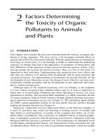
4.1 INTRODUCTION
In Chapter 3, the distribution of environmental chemicals through compartments of
the gross environment was related to the chemical factors and processes involved, and
models for describing or predicting environmental fate were considered. In the early
sections of the present chapter, the discussion moves on to the more complex question
of movement and distribution in the living environment—within individuals, com-
munities, and ecosystems—where biological as well as physical and chemical factors
come into play. The movement of chemicals along food chains and the fate of chemi-
cals in the complex communities of sediments and soils are basic issues here.
Ecotoxicology deals with the study of the harmful effects of chemicals in ecosys-
tems. This includes harmful effects upon individuals, although the ultimate concern
is about how these are translated into changes at the levels of population, community,
and ecosystem. Thus, in the concluding sections of the chapter, emphasis will move
from the distribution and environmental concentrations of pollutants to consequent
effects at the levels of the individual, population, community, and ecosystem. The
relationship between environmental exposure (dose) and harmful effect (response) is
fundamentally important here, and full consideration will be given to the concept of
biomarkers, which is based on this relationship and which can provide the means of
relating environmental levels of chemicals to consequent effects upon individuals,
populations, communities, and ecosystems.
4.2 MOVEMENT OF POLLUTANTS ALONG FOOD CHAINS
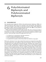
The pollutants of particular interest here are persistent organic chemicals—com-
pounds that have sufciently long half-lives in living organisms for them to pass
along food chains and to undergo biomagnication at higher trophic levels (see Box
4.1). Some compounds of lesser persistence, such as polycyclic aromatic hydrocar-

bons (PAHs) (Chapter 9), can be bioconcentrated/bioaccumulated at lower trophic
levels but are rapidly metabolized by vertebrates at higher levels. These will not be
discussed further here, where the issue is biomagnication with movement along the
© 2009 by Taylor & Francis Group, LLC
76 Organic Pollutants: An Ecotoxicological Perspective, Second Edition
entire food chain. The best studied examples of this are the organochlorines (OCs)
dieldrin and p,pb-DDE (see Chapter 5), and the PCBs (see Chapter 6), where concen-
trations in the tissues of predators of the highest trophic levels can be 10
4
–10
5
-fold
higher than in organisms at the lowest trophic levels. Other examples include poly-
chlorinated dibenzodioxin (PCDDs), polychlorinated dibenzofurans (PCDFs), and
some organometallic compounds (e.g., methyl mercury).
Biomagnication along terrestrial food chains is principally due to bioaccumu-
lation from food, the principal source of most pollutants (Walker 1990b). In a few
instances, the major route of uptake may be from air, from contact with contaminated
surfaces, or from drinking water. The bioaccumulation factor (BAF) of a chemical is
given by the following equation:
Concentration in organism/concentration in food = BAF
Biomagnication along aquatic food chains may be the consequence of biocon-
centration as well as bioaccumulation. Aquatic vertebrates and invertebrates can
absorb pollutants from ambient water; bottom feeders can take up pollutants from
sediments. The bioconcentration factor (BCF) of a chemical absorbed directly from
water is dened as
Concentration in organism/concentration in ambient water = BCF
One of the challenges when studying biomagnication along aquatic food chains
is establishing the relative importance of bioaccumulation versus bioconcentration.
The processes that lead to biomagnication have been investigated with a view to

developing predictive toxicokinetic models (Walker 1990b). When organisms are
continuously exposed to pollutants maintained at a fairly constant level in food and/
or in ambient water/air, tissue concentrations will increase with time until either (1) a
lethal concentration is reached and the organism dies or (2) a steady state is reached
when the rate of uptake of the pollutant is balanced by the rate of loss. The BCF or
BAF at the steady state is of particular interest and importance because (A) it rep-
resents the highest value that can be reached and therefore indicates the maximum
risk, (B) it is not time dependent, and (C) the rates of uptake and loss are equal,
thereby facilitating the calculation of the rate constants involved.
BCFs and BAFs measured before the steady state is reached have little value
because they are dependent on the period of exposure of the organism to the chemi-
cal, and thus may greatly underestimate the degree of biomagnication that is
possible. This statement should be qualied by the reservation that there may be
situations in which the duration of exposure cannot be long enough for the steady
state to be reached, for example, where the life span of an insect is very short. The
principal processes of uptake and loss by different types of organisms are indicated
in Table 4.1 (see also Box 4.2).
A rough indication of the relative importance of different mechanisms of uptake and
loss is given by a scoring system on the scale +−> ++++. Within each category of organ-
ism there will be differences between compounds in the relative importance of differ-
ent mechanisms, for example, due to differences in polarity and biodegradability.
© 2009 by Taylor & Francis Group, LLC
Distribution and Effects of Chemicals in Communities and Ecosystems 77
BOX 4.1 PERSISTENT ORGANIC POLLUTANTS (POPS)
A list of hazardous environmental chemicals, sometimes referred to as
the “dirty dozen,” has been drawn up by the United Nations Environment
Programme (UNEP). These are:
POP Year of Introduction Classification
Aldrin 1949 Insecticide
Chlordane 1945 Insecticide

DDT 1942 Insecticide
Dieldrin 1948 Insecticide
Endrin 1951 Insecticide and rodenticide
Heptachlor 1948 Insecticide
Hexachlorobenzene 1945 Fungicide
Mirex 1959 Insecticide
Toxaphene 1948 Insecticide and acaricide
PCBs 1929 Various industrial uses
Dioxins 1920s By-products of combustion, for example,
of plastics, PCBs
Furans 1920s By-products of PCB manufacture
The selection of these compounds was made on the grounds of their tox-
icity, environmental stability, and tendency to undergo biomagnication; the
intention was to move toward their removal from the natural environment. In
the REACH proposals of the European Commission (EC; published in 2003),
a similar list of 12 POPs was drawn up, the only differences being the inclusion
of hexachlorobiphenyl and chlordecone, and the exclusion of the by-products,
dioxins, and furans. The objective of the EC directive is to ban the manufac-
ture or marketing of these substances. It is interesting that no fewer than eight
of these compounds, which are featured on both lists, are insecticides.
TABLE 4.1
Principal Mechanisms of Uptake and Loss for Lipophilic Compounds
Mechanisms of Uptake Mechanisms of Loss
Habitat/Type of
Organism Diffusion From Food
From
Ingested Water Diffusion Metabolism
Aquatic
Mollusks ++++ + ++++
Fish ++++

+n +++
++++
+n +++
Terrestrial
Vertebrates ++++ < ++ ++++
© 2009 by Taylor & Francis Group, LLC
78 Organic Pollutants: An Ecotoxicological Perspective, Second Edition
BOX 4.2 MODELS FOR BIOCONCENTRATION
AND BIOACCUMULATION
As indicated in Table 4.1, aquatic mollusks present a relatively simple picture
because they have little capacity for biotransformation of organic pollutants,
the principal mechanism of both uptake loss being diffusion. It is not sur-
prising, therefore, that bioconcentration factors (BCFs) for diverse lipophilic
compounds, measured at the steady state, are related linearly to log K
ow
val-
ues (Figure 4.1). Thus, the more hydrophobic a compound is, the greater the
tendency to partition from water into the lipids of the mollusk. The relation-
ship shown in Figure 4.1 has been demonstrated in several species of aquatic
mollusks, including the edible mussel (Mytilus edulis), the oyster (Crassostrea
virginica), and soft clams (Mya arenaria) (Ernst 1977). A similar relationship
has also been found with rainbow trout and other sh for some pollutants. On
the other hand, some organic pollutants do not t the model well (Connor 1983).
It seems probable that some compounds that are metabolized relatively rapidly
by sh will be eliminated faster than would be expected if diffusion were the
only process involved (Walker 1987). Such compounds would not be expected
to follow closely a model for BCF based on K
ow
alone. This point aside, K
ow

values can give a useful prediction of BCF values at the steady state for lipo-
philic pollutants in aquatic invertebrates. A great virtue of the approach is that
K
ow
values are easy and inexpensive to measure or predict (Connell 1994).
Other more complex and sophisticated models have been developed for sh
(see, for example, Norstrom et al. 1976) but are too time-consuming/expensive
to be used widely in environmental risk assessment where cost-effectiveness
is critically important. Modeling for bioaccumulation by terrestrial animals
presents greater problems, and BAFs cannot be reliably predicted from K
ow
values (Walker 1987). For example, benzo[a]pyrene and dieldrin have log K
ow
values of 6.50 and 5.48, respectively, but their biological half-lives range from
a few hours in the case of the former to 10 –369 days for the latter. Endrin
is a stereoisomer of dieldrin with a similar K
ow
, but has a half-life of only 1
day in humans, compared with 369 days in the case of dieldrin. These large
differences in persistence have been attributed to differences in the rate of
metabolism by P450-based monooxygenases (Walker 1981). Effective predic-
tive models for bioaccumulation of strongly lipophilic compounds by terrestrial
animals need to take account of rates of metabolic degradation. This is not a
straightforward task and would require the sophisticated use of enzyme kinet-
ics to be successful. In one model, it has been suggested that Lineweaver–Burke
plots for microsomal metabolism might be used to predict BAF values in the
steady state (Walker 1987) (Figure 4.2). In principle, when an animal ingests a
lipophilic compound at a constant rate in its food, a steady state will eventually
be reached where the rate of intake of the compound is balanced by the rate of
its metabolism. It is assumed that the rate of loss of the unchanged compound

by direct excretion is negligible. Primary metabolic attack upon many highly
© 2009 by Taylor & Francis Group, LLC
Distribution and Effects of Chemicals in Communities and Ecosystems 79
The main points to bring out are as follows:
1. The uptake and loss by exchange diffusion is important for aquatic organ-
isms but not for terrestrial ones.
2. Metabolism is the main mechanism of loss in terrestrial vertebrates, but is
less important in sh, which can achieve excretion by diffusion into ambi-
ent water.
3. Most aquatic invertebrates have very little capacity for metabolism; this is
particularly true of mollusks. Crustaceans (e.g., crabs and lobsters) appear
to have greater metabolic capability than mollusks (see Livingstone and
Stegeman 1998; Walker and Livingstone 1992).
The balance between competing mechanisms of loss in the same organism depends
on the compound and the species in question. In sh, for example, some compounds
lipophilic compounds (e.g., polyhalogenated aromatic compounds and PAHs)
takes place predominantly in the endoplasmic reticulum, particularly that of the
liver in vertebrates. Thus, microsomes (especially hepatic microsomes of verte-
brates) can serve as model systems for measuring rates of enzymic detoxication.
Lineweaver–Burke and similar metabolic plots can relate concentrations of pol-
lutants in microsomal membranes to rates of metabolism. In the steady state,
rate of intake of chemical should equal rate of metabolism in the membranes
of the endoplasmic reticulum. The concentration of the chemical required in
the membranes to give this balancing metabolic rate can be estimated from the
Lineweaver–Burke plot. The necessary balancing metabolic rate can be calcu-
lated from the dened rate of intake in food, and then the microsomal concen-
tration that will give this rate can be read from the plot. Thus, the concentration
in endoplasmic reticulum can be compared to the dietary concentration to give
an estimate of BAF. Estimates can also be made of BAF for the liver or the
whole body if approximate ratios of concentrations of chemical in different

compartments of the body when at the steady state are known.
Log K
ow
Log BCF
FIGURE 4.1 Relationship of BCF to log K
ow
values.
© 2009 by Taylor & Francis Group, LLC
80 Organic Pollutants: An Ecotoxicological Perspective, Second Edition
that are good substrates for monooxygenases, hydrolases, etc., can be metabolized
relatively rapidly even though they, as a group, have relatively low metabolic capac-
ity (Chapter 2). So, in this case metabolism as well as diffusion is an important fac-
tor determining rate of loss. By contrast, many polyhalogenated compounds are only
metabolized very slowly by sh, so metabolism does not make a signicant contribu-
tion to detoxication, and loss by diffusion is the dominant mechanism of elimination.
Some further aspects of detoxication by sh need to be briey mentioned. When
sh inhabit polluted waters, exchange diffusion occurs until a steady state is reached,
and no net loss will occur by this mechanism unless the concentration in water falls.
When a recalcitrant pollutant is acquired from prey, digestion can lead to the tissue
levels of that pollutant temporally exceeding those originally existing while in the
steady state. Here, diffusion into the ambient water may provide an effective excre-
tion mechanism in the absence of effective metabolic detoxication. Seen from an
evolutionary point of view, the requirements of sh for metabolic detoxication would
appear to have been limited on the grounds that loss by diffusion would often have
prevented tissue levels becoming too high. The poor metabolic detoxication sys-
tems of sh relative to those of terrestrial omnivores and herbivores are explicable
on these grounds (Chapter 2). However, the advent of refractory organic pollutants,
which combine high toxicity with high lipophilicity, has exposed the limitations of
existing detoxication systems of sh. The very high toxicity of compounds such as
dieldrin and other cyclodiene insecticides to sh was soon apparent, with sh kills

occurring at very low concentrations in water (see Chapter 5) and metabolically
resistant strains of sh being reported in polluted rivers such as the Mississippi.
Gut
Liver
Peripheral
tissues
Redistribution
Metabolism and
excretion
(a) (b)
R
U
C
L
R
M
1
K
m
1
V
max
1
v
1
s
FIGURE 4.2 (a) A bioaccumulation model for terrestrial organisms. A kinetic model for
liver. R
U
, rate of uptake from the gut; R

M
, rate of metabolism in liver; C
L
, concentration of
pollutant in liver. The arrows indicate the routes of transfer of pollutant within the animal.
The rates of uptake and metabolism are expressed in terms of kilograms of body weight. The
nal elimination of water-soluble products (metabolites and conjugates) is in the urine. (b)
Lineweaver–Burke plot to estimate the bioaccumulation factor; V
max
and v are expressed as
milligrams of pollutant metabolized per kilogram of body weight per day; S is expressed as
the concentration of pollutant, ppm by weight (either in terms of grams of liver or milligrams
of hepatic microsomal protein) (from Walker 1987).
© 2009 by Taylor & Francis Group, LLC
Distribution and Effects of Chemicals in Communities and Ecosystems 81
More rapid elimination was needed than could be provided by passive diffusion in
order to prevent tissue concentrations reaching toxic levels.
Some models for predicting bioconcentration and biomagnication are presented
in Box 4.1.
4.3 FATE OF POLLUTANTS IN SOILS AND SEDIMENTS
Regarding soils, a central issue is the persistence and movement of pesticides that are
widely used in agriculture. Many different insecticides, fungicides, herbicides, and
molluscicides are applied to agricultural soils, and there is concern not only about
effects that they may have on nontarget species residing in soil, but also on the pos-
sibility of the chemicals nding their way into adjacent water courses.
Soils are complex associations between living organisms and mineral particles.
Decomposition of organic residues by soil microorganisms generates complex
organic polymers (“humic substances” or simply “soil organic matter”) that bind
together mineral particles to form aggregates that give the soil its structure. Soil
organic matter and clay minerals constitute the colloidal fraction of soil; because

of their small size, they present a large surface area in relation to their volume.
Consequently, they have a large capacity to adsorb the organic pollutants that con-
taminate soil. Within a freely draining soil there are air channels and soil water,
the latter being closely associated with solid surfaces. Depending on their physical
properties, organic compounds become differentially distributed between the three
phases of the soil, soil water, and soil air.
Hydrophobic compounds of high K
ow
become very strongly adsorbed to soil col-
loids (Chapter 3, Section 3.1), and consequently tend to be immobile and persistent.
OC insecticides such as DDT and dieldrin are good examples of hydrophobic com-
pounds of rather low vapor pressure that have long half-lives, sometimes running
into years, in temperate soils (Chapter 5). Because of their low water solubility and
their refractory nature, the main mechanism of loss from most soils is by volatiliza-
tion. Metabolism is limited by two factors: (1) being tightly bound, they are not freely
available to enzymes of soil organisms, which can degrade them, and (2) they are, at
best, only slowly metabolized by enzyme systems. Because of strong adsorption and
low water solubility, there is little tendency for them to be leached down the soil pro-
le by percolating water. The degree of adsorption, and consequently the persistence
and mobility, is also dependent on soil type. Heavy soils, high in organic matter and/
or clay, adsorb hydrophobic compounds more strongly than light sandy soils, which
are low in organic matter. Strongly lipophilic compounds are most persistent in heavy
soils. When OC insecticides are rst incorporated into soil, they are lost relatively
rapidly, mainly due to volatilization, before they become extensively adsorbed to soil
colloids (Figure 4.3). With time, however, most residual OC insecticide becomes
adsorbed, and subsequently there is a period of very slow exponential loss.
In marked contrast to hydrophobic compounds, more polar ones tend to be less
adsorbed and to reach relatively high concentrations in soil water. Phenoxyalkanoic
acids such as 2,4-D and MCPA are good examples (Figure 4.3). Their half-lives in soil
are measured in weeks rather than years, and they are more mobile than OC insec-

ticides in soils. When rst applied they are lost only slowly. After a lag period of a
© 2009 by Taylor & Francis Group, LLC
82 Organic Pollutants: An Ecotoxicological Perspective, Second Edition
few days, however, they disappear very rapidly as a consequence of metabolism by
soil microorganisms. This has been explained on the grounds that it takes time for
a buildup in numbers of strains of microorganisms that can metabolize them; these
microorganisms use the herbicides as an energy source. It has also been suggested that
the lag period relates to the time it takes for enzyme induction to occur. Whatever the
explanation, soils treated with these compounds stay enriched for a period, and further
additions of the original compounds will be followed by rapid metabolism without
a lag phase. If, however, the soils are untreated for a long period, they will revert to
their original state and not show any enhanced capacity for degrading the herbicides.
An important difference from the OC insecticides and related hydrophobic pollutants
is that, because of their polarity and water solubility, they are freely available to the
microorganisms that can degrade them. Interestingly, the phenoxyalkanoic acid 2,4,5-T
is more persistent than either 2,4-D or MCPA. With three substituted chlorines in its
phenyl ring, it is metabolized less rapidly than the other two compounds, and it would
appear that metabolism is a rate-limiting factor determining rate of loss from soil.
It was long assumed that there is little tendency for most pesticides or other organic
pollutants to move through soil into drainage water. Indeed, this is to be expected
with intact soil proles. Hydrophobic compounds will be held back by adsorption,
whereas water soluble ones will be degraded by soil organisms. Some soils, how-
ever, depart from this simple model. Soils high in clay can crack and develop deep
ssures during dry weather. If rain then follows, pesticides, in solution or adsorbed
to mobile colloids, can be washed down through the ssures, to appear in neighbor-
ing drainage ditches and streams. This was found to happen with pesticides such as
carbofuran, isoproturon, and chlorpyrifos in the Rosemaund experiment conducted
in England during the period 1987–1993 (Williams et al. 1996).
0
0 10203040 506070 8090100

Days after Application
Time Following Application
(b)
(a)
20
Herbicide Concentration (ppm)
Log Concentration in Soil
40
60
80
100
120
Lag period
Lag period
2,4-D
MCPA
Period of rapid loss during
application and cultivation
and for a time afterwards
Concentration that would
have been found if all applied
material were retained by soil
Period of slo
w
exponential
loss
FIGURE 4.3 Loss of pesticides from soil. (a) Breakdown of herbicides in soil. (b) Dis-
appearance of persistent organochlorine insecticides from soils (from Walker et al. 2000).
© 2009 by Taylor & Francis Group, LLC
Distribution and Effects of Chemicals in Communities and Ecosystems 83

The inuence of polarity on movement of chemicals down through the soil prole
has been exploited in the selective control of weeds using soil herbicides (Hassall
1990). In general, the more polar and water soluble the herbicide, the further it will
be taken down into the soil by percolating water. Insoluble herbicides such as the
triazine compound simazine (water solubility, 3.5 ppm), remain in the rst few cen-
timeters of soil when applied to the surface. More water-soluble compounds such
as the urea herbicides diuron and monuron (water solubilities 42 ppm and 230 ppm,
respectively) are more mobile, and can move farther down the soil prole. Selective
weed control can be achieved in some deep-rooting crops by judicious selection from
this range of herbicides, so that the herbicide will only percolate far enough down
the soil prole to control surface rooting weeds without reaching the main part of
the root system of the crop (depth selection). Thus, when applied to the soil surface,
simazine should only be toxic to shallow rooting weeds and should not affect crops
that root farther down. Other more water-soluble herbicides can give weed control
to greater depths in situations where the rooting systems of the crops are sufciently
deep. When attempting depth selection in weed control, account needs to be taken
of soil type. Herbicides will move farther down the prole in the case of light sandy
soils than they will in heavy clays or organic soils.
Although the major concern about the fate of organic pollutants in soil has been
about pesticides in agricultural soils, other scenarios are also important. The dis-
posal of wastes on land (e.g., at landll sites) has raised questions about movement
of pollutants contained in them into the air or neighboring rivers or water courses.
The presence of polychlorinated biphenyls (PCBs) or PAHs in such wastes can be a
signicant source of pollution. Likewise, the disposal of some industrial wastes in
landll sites (e.g., by the chemical industry) raises questions about movement into air
or water and needs to be carefully controlled and monitored.
In certain respects, sediments resemble soils. Sediments also represent an asso-
ciation between mineral particles, organic matter, and resident organisms. The
main difference is that they are situated underwater and are, in varying degrees,
anaerobic. The oxygen level inuences the type of organisms and the nature of

biotransformations that occur in sediments. A feature with sediments, as with
soils, is the limited availability of chemicals that are strongly adsorbed. Again,
compounds with high K
ow
tend to be strongly adsorbed, relatively unavailable, and
highly persistent. There is much interest in the question of sediment toxicity and
the availability to bottom-dwelling organisms of compounds adsorbed by sedi-
ments (Hill et al. 1993). One case in point is pyrethroid insecticides (see Chapter
12), which are strongly retained in sediments on account of their high K
ow
values.
Because of their ready biodegradability, they are not usually biomagnied in the
higher trophic levels of aquatic food chains.
However, they are available to bottom-dwelling organisms low in the food chain.
Questions are asked about the possible long-term buildup of pyrethroids in sedi-
ments and their effects on organisms in lower trophic levels.
© 2009 by Taylor & Francis Group, LLC
84 Organic Pollutants: An Ecotoxicological Perspective, Second Edition
4.4 EFFECTS OF CHEMICALS UPON INDIVIDUALS—
THE BIOMARKER APPROACH
Until now this narrative has been concerned with questions about the movement and
distribution of chemicals in the living environment, a topic that relates to the eld of
toxicokinetics in classical toxicology, although on a much larger scale. It is now time
to move to a consideration of the effects that chemicals may have upon living organ-
isms, which relates to the area of toxicodynamics in classical toxicology. Effects
upon individuals will be discussed before dealing with consequent changes at the
higher levels of biological organization—population, community, and ecosystem.
Measuring effects of chemicals upon free-living individuals in the natural envi-
ronment is not an easy matter. Mobile animals need to be captured so that samples
of tissues can be taken for analysis, but this is often difcult to do in a properly

controlled way in the eld. It is easier to obtain samples from sedentary species (e.g.,
mollusks or plants) or of eggs in the case of birds, reptiles, and some invertebrates.
All too often sampling is destructive, which raises problems of experimental design
and statistical evaluation of results. In principle, measuring behavioral effects of
chemicals is an attractive option, but this can be hard to achieve in practice because
of the difculty of making reliable measurements in the eld. The problems of sam-
pling can, to some extent, be circumvented by deploying indicator species that have
been maintained in a “clean” environment into the eld. Thus, control sh from the
laboratory can be held in cages in contaminated waters and samples taken from them
after periods of exposure to pollutants. Uncontaminated birds’ eggs can be intro-
duced into the nests of birds of the same species that are breeding in a polluted area.
In this way, changes caused by pollutants can be measured and evaluated.
Problems of sampling aside, the success of any strategy of this kind depends on
the availability of reliable tests that can measure harmful effects of chemicals under
eld conditions. Reference has already been made to biomarkers (Chapter 2, Box
2.2). In the following account they are dened as “biological responses to environ-
mental chemicals at the individual level or below, which demonstrate a departure
from normal status.” This denition includes biochemical, physiological, histologi-
cal, morphological, and behavioral changes, but does not extend to changes at higher
levels of organization. Changes at population, community, or ecosystem level are
regarded instead as bioindicators.
The concept of biomarkers is illustrated in Figure 4.4. As the dose of a chemical
increases, the organism moves from a state of homeostasis to a state of stress. With fur-
ther increases in dose, the organism enters rst the state of reversible disease, and even-
tually the state of irreversible disease, which will lead to death. In concept, all of these
stages can be monitored by biomarker assays (lower part of conceptual diagram).
Some biomarker responses provide evidence only of exposure and do not give
any reliable measure of toxic effect. Other biomarkers, however, provide a measure
of toxic effects, and these will be referred to as mechanistic biomarkers. Ideally, bio-
marker assays of this latter type monitor the primary interaction between a chemical

and its site of action. However, other biomarkers operating “down stream” from the
original toxic lesion also provide a measure of toxic action (see Figure 14.3 in Chapter
14), as, for instance, in the case of changes in the transmission of action potential
© 2009 by Taylor & Francis Group, LLC
Distribution and Effects of Chemicals in Communities and Ecosystems 85
following the interaction of DDT or pyrethroids with Na
+
channels, although these
are changes that may also be caused by the operation of other toxic mechanisms.
These will also be treated as mechanistic biomarkers in order to distinguish them
from other responses that are only biomarkers of exposure (e.g., the induction of
certain enzymes that can occur at low levels of exposure before any toxic effects are
manifest). Mechanistic biomarkers (see Table 4.2 for examples) have potential for
measuring adverse effects of chemicals in the eld—effects that may be translated
into changes at the population level and above.
Healthy
Disease
Incurable
Curable
Health status
Reversible
Irreversible
Stressed
Intensity of Biomarker Response
Physiological Condition
Pollutant Concentration
Homeostasis Compensation Death
c
r
h

B1
B2
B3
B4
B5
Noncompensation
FIGURE 4.4 Relationship between exposure to pollutant, health status, and biomarker
responses. Upper curve shows the progression of the health status of an individual as expo-
sure to pollutant increases; h, the point at which departure from the normal homeostatic
response range is initiated; c, the limit at which compensatory responses can prevent develop-
ment of overt disease; r, the limit beyond which pathological damage is irreversible by repair
mechanisms. The lower graph shows the response of ve different hypothetical biomarkers
used to assess the health of the individual. (Reproduced from Depledge et al. 1993. With
permission from Springer-Verlag.)
© 2009 by Taylor & Francis Group, LLC
86 Organic Pollutants: An Ecotoxicological Perspective, Second Edition
Of the examples given, brain cholinesterase inhibition has been frequently mea-
sured in eld studies involving OP insecticides and when investigating cases of poi-
soning on agricultural land (see Chapter 10). A number of studies on sh, rodents,
and birds in the eld and/or in the laboratory give evidence for a range of sublethal
neurotoxic and behavioral effects of OP insecticides when brain acetylcholinesterase
inhibition is in the range 40–50%—before the appearance of severe toxic manifesta-
tions and death (see Chapters 10 and 16). A few OP compounds cause delayed neu-
ropathy in mammals and birds, and this has been related to inhibition of neuropathy
target esterase (NTE). Symptoms of this type of poisoning appear after aging of the
inhibited enzyme occurs (Chapter 10). Warfarin and related anticoagulant rodenti-
cides act as competitive antagonists of vitamin K at binding sites for this cofactor in
the liver and consequently inhibit the carboxylation of precursors of blood-clotting
proteins (Chapter 11). Thus, undercarboxylated Gla proteins are released into the
blood. After a period of time (usually 5 days or more) the blood becomes depleted

of normal clotting proteins and loses its capacity to coagulate. A valuable biomarker
assay involves the measurement of levels of undercarboxylated clotting protein in the
blood by immunochemical determination. An increase of this nonfunctional protein
in the blood provides a measure of the toxic process that leads to hemorrhaging and
death—although it does not measure the primary interaction between rodenticide
and the vitamin K binding site in the liver. Certain metabolites of coplanar PCBs
such as 4-OH, 3,3b,4,4b-TCB can compete with thyroxine (T4) for binding sites on
the protein transthyretin in blood. This interaction leads to the breaking apart of
TABLE 4.2
Some Mechanistic Biomarker Assays
Assay Chemicals Secondary Effects
Chapter
in This Text
Brain acetylcholinesterase
inhibition
OP and carbamate
insecticides
Acetylcholine buildup in
synapse and synaptic
block
10, 16
Inhibition of neuropathy
target esterase (NTE) in
mammals
Mipafox, DFP, leptophos,
TOCP, acetamidophos
Nerve degeneration 10, 16
Undercarboxylated Gla
proteins in blood of
vertebrates

Warfarins and
superwarfarins
Hemorrhaging 11
Occupancy of retinol
binding site of
transthyretin in vertebrate
blood
4-OH, 3,3b,4,4b
tetrachlobiphenyl and
related PCB metabolites
Reduced levels of retinol
and thyroxine (T4) in
blood
6
Eggshell thinning in birds
p,pb-DDE
Egg breakage 5
Imposex in dog whelk Tributyl tin Infertility of females 8
© 2009 by Taylor & Francis Group, LLC
Distribution and Effects of Chemicals in Communities and Ecosystems 87
the protein and the loss of thyroxine and retinol from the blood. Here, measure-
ment of the reduction of binding of thyroxine to transthyretin provides the basis for
a mechanistic biomarker assay that reports changes at the site of action caused by
these metabolites of PCBs (Brouwer et al. 1990, 1998). p,pb-DDE causes eggshell
thinning in birds by retarding the uptake of Ca
++
across the wall of the shell gland
(Chapter 5). There is still some uncertainty about the exact mechanism by which
p,pb-DDE retards the movement of Ca
++

into the shell gland, although both inhibi-
tion of calcium ATPase and changes in prostaglandin levels have been implicated
(Lundholm 1997). Again, the secondary effect—thinning of the eggshell—provides
a good monitor of the toxic process. Finally, imposex is a condition that can be
caused by tributyl tin (Chapter 8). It seems probable that the primary effect is to
inhibit the production of testosterone. This point aside, a convenient biomarker assay
measures the development of a penis by the female dog whelk that, when sufciently
large, blocks the oviduct and causes infertility. Once again, a biomarker assay pro-
vides a convenient measure of the toxic process.
In all of these examples it should be noted that the toxic process occurs through
different stages over a period of time. In some instances (e.g., delayed neuropathy
caused by some OPs, and hemorrhaging caused by warfarin) there may be a delay
of several weeks between initial exposure and the appearance of overt symptoms of
poisoning, which raises two issues. First, it emphasizes the importance of having
sensitive biomarkers that can provide early measures of intoxication before severe
toxicity occurs. Second, if we are to understand toxicity at a deeper level, the dif-
ferent stages in the process need to be understood and be readily measurable. These
issues will be returned to later in the text, especially in Chapters 15 and 16, when
consideration will be given to the development of new biomarker strategies, incorpo-
rating the omics, which have the potential to address both questions (Box 4.3).
A number of attributes are sought when developing biomarker assays. At a practi-
cal level, assays should be robust, inexpensive, and relatively easy for nonspecialists
to use. Unfortunately, some promising assays are really at the stage of being research
tools, only usable by experts with specialized apparatus. There is a need for user-
friendly kits (such as the diagnostic kits that are widely available to medical laborato-
ries) for use in nonspecialist laboratories with relatively simple apparatus. Specicity
is another desirable characteristic, in the sense of identifying a particular mechanism
of toxicity and, therefore, a particular class of organic pollutant. When dealing with
complex cases of pollution, it is extremely valuable to have biomarker assays that can
provide evidence of causal links between levels of particular pollutants (or classes

of pollutant) detected in the environment and associated harmful biological effects.
Examples of such biomarkers include imposex in dog whelks related to tributyl tin,
brain cholinestease inhibition in vertebrates caused by organophosphorous insecti-
cides, and eggshell thinning of some predatory birds caused by p,pb-DDE (Table 4.2).
Sensitivity is another desirable characteristic that can facilitate the early detection
of sublethal effects. The detection of later effects seen during the terminal stages of
poisoning is of less value.
© 2009 by Taylor & Francis Group, LLC
88 Organic Pollutants: An Ecotoxicological Perspective, Second Edition
In practice, all of these attributes are unlikely ever to be found in a single bio-
marker assay. However, the ultimate aim is to produce combinations of biomarker
assays that collectively can give an in-depth picture of the toxic process (Peakall and
Shugart 1993; Walker et al. 2006). In this way, the time-dependent changes follow-
ing the interaction of a pollutant with its site of action can be traced through different
levels of organization, progressing from the site of action itself through local cel-
lular disturbances to effects expressed at the level of the whole organism, including
behavioral effects—in other words, through the entire pathway of the toxic process.
Examples of biomarker assays operating at different levels are given in Table 4.2.
The recent development of “omics” technology should provide strong support to
this approach (Box 4.3). Microarray analysis, for instance, can give a time-related
sequence of gene responses that relate to the cellular changes of toxicity.
BOX 4.3 THE OMICS
Recent rapid technological advances have spawned a host of new terms that
have caused confusion not only to interested laypeople but even to members
of the scientic community. Many recently dened omics represent a case in
point. The term genome was proposed by Hans Winkler in 1920 to describe the
complete set of genes for a particular species (Snape et al. 2004; van Straalen
and Roelofs 2006). Much later the term genomics appeared in the title of a jour-
nal (see, for example, McKusick 1997). Genomics has been dened as the study
of how the genome translates into biological functions (Snape et al. 2004).

This denition of the term genomics is a broad one and includes both
structural and functional aspects. Other terms relating to gene function are
transcriptomics (study of the transcripts of DNA, principally mRNA), pro-
teomics (study of all the proteins of the cell), and metabolomics (the study of
metabolites) (van Straalen and Roelofs 2006). Other terms that have arisen are
toxicogenomics, which applies genomics to mammalian toxicology (Nuwaysir
et al. 1999), and ecotoxicogenomics, which applies genomics to ecotoxicology
(Snape et al. 2004). New techniques in these elds are necessarily underpinned
by sophisticated information technology.
In the present context, the techniques of genomics have great potential in
ecotoxicology, particularly as the basis of biomarker assays. DNA microarray
assays allow the measurement of changes in gene expression when organisms
are exposed to chemicals and other stressors (Burczynski 2003). In essence,
the products of gene expression (mRNA converted into cDNA) are measured
by hybridizing them to complementary sequences of DNA printed onto a glass
slide (microarray). After processing, genes that have increased their expres-
sion will be colored green, those that have decreased their expression will be
red, and the level of expression will be indicated by the intensity of the color.
In principle, the time-dependent response to a chemical of certain genes of
an entire genome can be measured. Such a sequence of gene responses can
be compared with the corresponding sequence of cellular responses to a toxic
© 2009 by Taylor & Francis Group, LLC
Distribution and Effects of Chemicals in Communities and Ecosystems 89
4.5 BIOMARKERS IN A WIDER ECOLOGICAL CONTEXT
From an ecological point of view, chemicals can be seen as constituting one class of
agents that stress biological systems (“stressors”) (Van Straalen 2003). As we have
seen, organic chemicals that have harmful effects upon living organisms may be
naturally occurring as well as human made, and both may contribute to “chemical
stress” (Chapter 1). Other stressors include extremes of temperature, acidity, humid-
ity, and levels of inorganic ions not usually regarded as toxic (e.g., nitrate, phosphate,

etc.). In an ideal world, the stress caused by all of these factors should be taken into
account when considering the state—healthy or otherwise—of individuals, popu-
lations, communities, and ecosystems. It may even be argued that, in the ultimate
analysis, ecotoxicology is part of stress ecology (Van Straalen 2003).
However, there are a number of issues here. In the rst place, stress itself is a
somewhat nebulous concept, and there is continuing debate about how it should be
dened. Second, even with the benet of multivariate statistics and the techniques of
bioinformatics, measuring stress from all sources in a meaningful way is dauntingly
complex and may not be realizable in practice.
So far as the discipline of ecotoxicology goes, there have been a number of cases
where organic pollutants were shown to be the principal or sole cause of population
declines in the natural environment, and these are described in the chapters that
chemical measured by mechanistic biomarker assays, as described in this sec-
tion and in later parts of this text (note especially Chapters 15 and 16).
Unfortunately, as with many exciting new areas of science, ideas are much
easier to conceive than to deliver. There are many difculties both in the
execution and—not least—the interpretation of results from toxicogenomic
assays. There has been a serious problem with regard to controlling data qual-
ity. Indeed, some journals, for example, Nature, have adopted strict guidelines
on data quality when assessing papers submitted to them for publication on
this subject. Also, the value of genomic data in ecotoxicology needs to be seen
in context. Genotoxic compounds represent a rather small proportion of the
pollutants that are known to have had serious ecotoxicological effects, as will
be apparent from the pages that follow. Most primary toxic interactions—or
their immediate knock-on effects—are not at the level of the gene. Changes in
gene expression bear testimony to toxic disturbances in the organism—to the
disturbance of cellular processes, to the disruption of neurotransmission, to
the ability of blood to clot, etc. They do not provide direct measures of the ini-
tial toxic interactions or the consequent cellular disturbances. Thus, genomic
techniques have great potential when used in combination with mechanistic

biomarker assays that measure the toxic process itself. They also have poten-
tial for screening where toxic effects are suspected in the environment. The
pattern of genomic response may give critical evidence about the mode of
toxic action that operates when pollution occurs.
© 2009 by Taylor & Francis Group, LLC
90 Organic Pollutants: An Ecotoxicological Perspective, Second Edition
follow. These have included cases where the recovery of populations followed the
reduction of pollutant levels in the environment. Examples include the declines of
predatory birds caused by cyclodiene insecticides and p,pb-DDE, and the decline
of dog whelks caused by tributyl tin. Here, other stress factors were evidently not
implicated in either the declines or the recoveries. However, now that action has
been taken to rectify problems such as these in most parts of the world, the effects of
pollutants are less easy to detect and may increasingly need to be seen in relation to
stress factors more generally.
From a toxicological point of view, stress needs to be seen in relation to the toxic
process as a whole (Figure 4.4). As the dose of a toxicant increases, organisms move
from a homeostatic state through a stressed state to a reversible disease state, before
nally reaching an irreversible disease state. Thus, although the impact of stress
needs to be taken into consideration in the early stages of intoxication, the more
serious effects in terms of health tend to come later when moving beyond stress to
fundamental disturbances of function that may lead to starvation, infertility, and
death. Indeed, it was effects of the latter kind that led to the population declines
referred to previously.
4.6 EFFECTS OF CHEMICALS AT THE POPULATION LEVEL
4.6.1 P
OPULATION DYNAMICS
In environmental risk assessment, the objective is to establish the likelihood of a
chemical (or chemicals) expressing toxicity in the natural environment. Assessment
is based on a comparison of ecotoxicity data from laboratory tests with estimated
or measured exposure in the eld. The question of effects at the level of population

that may be the consequence of such toxicity is not addressed. This issue will now
be discussed.
Toxic effects upon individuals in the eld may be established and quantied in a
number of assays. Lethal effects can be assessed by collecting and counting corpses
found in the eld following the application of a chemical, as in eld trials with new
pesticides. This is an imprecise technique because many individual casualties will
escape detection, especially with mobile species such as birds. With very stable pol-
lutants such as dieldrin, heptachlor epoxide, p,pb-DDT, and p,pb-DDE, the determina-
tion of residues in carcasses found in the eld can provide evidence of lethal toxicity
in the eld. Such data may also be used to obtain estimates of the effects of chemi-
cals upon mortality rates of eld populations, which can then be incorporated into
population models (see Chapter 5, Section 5.3.5.1). Mechanistic biomarker assays
can also be used to quantify toxic effects in the eld. Even when investigating cases
of lethal poisoning, relatively stable biomarker assays such as cholinesterase inhibi-
tion may be used to establish the cause of death so long as carcasses are relatively
fresh. Of particular interest is the use of biomarker assays to monitor the effects
of chemicals on living organisms in the eld. Here, biomarker assays can provide
measures of sublethal toxic effects. Ideally, these should be nondestructive, to allow
serial sampling of individuals.
© 2009 by Taylor & Francis Group, LLC
Distribution and Effects of Chemicals in Communities and Ecosystems 91
The present section will be limited to the question of effects on populations that
are a direct consequence of toxicity to individuals, whether lethal or sublethal. The
problem of indirect effects have been touched upon when discussing effects at the
level of a community or ecosystem (Section 4.5). The important point to emphasize
at this early stage, though, is that a reduction in numbers of one species caused by
a toxic chemical can have knock-on effects on populations of other species in a
community or an ecosystem. The state of a population can be expressed in terms of
numbers (population dynamics) or genetic composition (population genetics). This
section will deal with questions relating to population dynamics; the next will deal

with population genetics.
The population density of animals in the natural environment is far from con-
stant. Seasonal uctuations are normal, with an increase in numbers during and
immediately after breeding, but a decline between this time and the next breed-
ing occasion. In temperate climates, most breeding occurs during the warm season,
when food is most readily available. Numbers fall during the cold season, when there
is a shortage of food. Given these complications, it is understandable that ecologists
and ecotoxicologists are particularly interested in the growth rate of populations (r).
Population growth rate is dened as the population increase per unit time divided by
the number of individuals in the population (see Chapter 12, Walker et al. 2000 and
Gotelli 1998). Population growth rate may be positive, negative, or zero. When r =
0, the rates of recruitment and loss are equal, and the population density in the eld
represents the carrying capacity. In the eld, population numbers are determined
by, among other things, density-dependent factors such as availability of food, water,
or breeding sites. Population density in the eld cannot exceed, for any appreciable
period, the carrying capacity. When investigating the effects of factors such as pol-
lutants on population numbers, an important question is whether they bring popula-
tion numbers below the carrying capacity. A pollutant may reduce survivorship or
reproductive success, but this does not necessarily reduce population numbers below
that which would normally be maintained by density-dependent factors.
In general, it can be stated that the population density of an animal depends on
the balance between the rate of recruitment and the rate of mortality. In the context
of ecotoxicology, the inuence of pollutants upon either of these factors is of funda-
mental interest and importance. When a population is at or near its carrying capacity,
these two factors are in balance, and the critical question about the effects of pollut-
ants is whether they can adversely affect this balance and bring a population decline.
The population growth rate of an organism can be calculated from the Euler–
Lotka equation
1 = 1/2n
1

l
1
e
−rt
1
+1/2n
2
l
2
e
−rt
2
+1/2 n
3
l
3
e
−rt
3
, etc.
where t
1
equals age of rst breeding, t
2
equals age of second breeding, t
3
equals
age of third breeding, etc.
l
1

is the probability of female surviving to the age of rst breeding, l
2
, the
probability of reaching age of second breeding, etc.
n
1
is the number of offspring produced at the rst breeding, n
2
, the number
of offspring produced at the second breeding, etc.
© 2009 by Taylor & Francis Group, LLC
92 Organic Pollutants: An Ecotoxicological Perspective, Second Edition
In predicting the effects of a pollutant on population growth rate, the effects of the
chemical on the values of t, l, and n are of central interest. Chemical residue data and
biomarker assays that provide measures of toxic effects are relevant here because
they can, in concept, be used to relate the effects of a chemical upon the individual
organism to a population parameter such as survivorship or fecundity (Figures 4.5
and 4.6). Examples of this are discussed in the second part of the text, including
the reduction of survivorship of sparrow hawks caused by dieldrin (Chapter 5), the






FIGURE 4.5 Schematic diagram of the relationship between biomarker response and change
in population parameter.
Conc. to
which
Organism

Exposed
Responses
Tissue
Conc.
Receptor
Occupancy
Local
Response
Response
Whole
Organism
Response
Population
FIGURE 4.6 Schematic diagram illustrating response to pollutants at different levels of
biological organization. The threshold tissue concentrations, for which no response is mea-
surable, are indicated by arrows for each of the biological responses. These thresholds tend to
increase with movement toward higher levels of biological organization.
© 2009 by Taylor & Francis Group, LLC
Distribution and Effects of Chemicals in Communities and Ecosystems 93
reduction in breeding success of raptors caused by p,pb-DDE (Chapter 5), and the
reduction in fecundity of dog whelks caused by TBT (Chapter 8). The measurement
of responses of free-living organisms to pollutants in the eld using appropriate bio-
marker assays can be a prelude to estimating the consequent effects upon t, l, or n
from graphs of the type shown in Figure 4.5. The estimated values can then be incor-
porated into equations such as the one shown previously to predict the effects of the
chemical on r. Such models can be tested in eld studies or in mesocosm studies to
establish their validity. It is also possible, in concept, to utilize biomarker responses
determined in the laboratory to predict the effects at the population level of known or
predicted exposures to particular chemicals in the eld. In the simplest case, such an
approach would assume that the relationship between the biomarker responses and

the consequent change in the population parameter would be similar in the eld to
that in the laboratory. However, this approach would need to be rigorously tested in
the eld because the relationship might be substantially different between laboratory
and eld.
The development of models incorporating biomarker assays to predict the effects
of chemicals upon parameters related to r has obvious attractions from a scientic
point of view and is preferable, in theory, to the crude use of ecotoxicity data cur-
rently employed in procedures for environmental risk assessment. However, the
development of this approach would involve considerable investment in research,
and might prove too complex and costly to be widely employed in environmental
risk assessment.
4.6.2 POPULATION GENETICS
As explained in Chapter 1, the toxicity of “natural” xenobiotics has exerted a selec-
tion pressure upon living organisms since very early in evolutionary history. There
is abundant evidence of compounds produced by plants and animals that are toxic to
species other than their own and which are used as chemical warfare agents (Chapter
1). Also, as we have seen, wild animals can develop resistance mechanisms to the
toxic compounds produced by plants. In Australia, for example, some marsupials
have developed resistance to naturally occurring toxins produced by the plants upon
which they feed (see Chapter 1, Section 1.2.2).
It is only very recently that organic compounds synthesized by humans have
begun to exert a selection pressure upon natural populations, with the consequent
emergence of resistant strains. Pesticides are a prime example and will be the princi-
pal subject of the present section. It should be mentioned, however, that other types
of biocides (e.g., antibiotics and disinfectants) can produce a similar response in
microbial populations that are exposed to them.
The large-scale use of pesticides commenced in developed countries after the
Second World War. In due course, they came to be more widely used in develop-
ing countries, notably for the large-scale control of important vectors of disease
such as malarial mosquitoes and tsetse ies. With the continuing use of pesticides,

problems of resistance began to emerge. The emergence of strains of pest spe-
cies possessing genes that confer resistance was an inevitable consequence of the
© 2009 by Taylor & Francis Group, LLC
94 Organic Pollutants: An Ecotoxicological Perspective, Second Edition
continuing selection pressure of the pesticides. Indeed, this can be seen to mirror
the development of defense systems toward natural toxins much earlier in evolution-
ary history. It is highly probable that many of the defense systems now emerging in
resistant strains were originally developed to combat natural toxins (e.g., P450 forms
of some resistant strains of insects).
The development of resistant strains of pest species of insects has been intensively
studied for sound economic reasons, and there are many good examples. For further
information, see Brown (1971), Georghiou and Saito (1983), McCaffery (1998), and
Oppenoorth and Welling (1976). Some examples of mechanisms of insect resistance
are given in Table 4.3.
The levels of resistance (SR values) developed by insects toward insecticides in
the eld can be as high as several hundredfold relative to susceptible strains of the
same species. Such high levels of resistance usually lead to loss of effective control
of the pest. Broadly speaking, resistance mechanisms are of two kinds: (1) those
depending on toxicokinetic factors such as reduced uptake, increased metabolism,
or increased storage, and (2) those depending on toxicodynamic factors, principally
making alterations in the site of action, which lead to decreased sensitivity to the
insecticide. These two kinds of mechanism are considered in the following text.
Resistance mechanisms associated with changes in toxicokinetics are pre-
dominately cases of enhanced metabolic detoxication. With readily biodegrad-
able insecticides such as pyrethroids and carbamates, enhanced detoxication by
P450-based monooxygenase is a common resistance mechanism (see Table 4.3).
TABLE 4.3
Examples of Resistance of Insects to Insecticides
Insecticide Species Strain (RF) Mechanism Comment
Cypermethrin

(cis-isomers)
Heliothis
virescens
PEG 87
(70,000+)
P450 (major)
Altered NaCh
(minor)
Resistance
sensitive to PBO
Cypermethrin
(cis-isomers)
H. virescens Field strains
(85–315)
Altered NaCh
(principal)
Little metabolic
resistance
Parathion
Methyl parathion
H. virescens Field strains Altered Ch-ase
OPs Myzus persicae Resistant clones
(85–315)
Enhanced
B esterase
Multiple copies of
gene
Cyclodienes H. virescens Field strains Altered GABA
DDT Musca
domestica

Many strains Enhanced
DDT-ase
DDTase inhibitors
reduce resistance
Carbamates Several Various (< 200) P450 PBO reduces
resistance
Note: NaCh = sodium channel; RF = resistance factor, which is LD
50
resistant strain/LD
50
susceptible
strain; GABA = gamma amino butyric acid receptor; PBO = piperonyl butoxide.
Sources: McCaffery (1998), Oppenoorth and Welling (1976), Devonshire (1991), Devonshire and
Field (1991).
© 2009 by Taylor & Francis Group, LLC
Distribution and Effects of Chemicals in Communities and Ecosystems 95
The existence of this type of resistance can often be established by toxicity stud-
ies with synergists. Inhibitors of P450 forms such as piperonyl butoxide (PBO)
can substantially reduce the level of resistance shown by the resistant strains.
OP resistance is sometimes due to enhanced esterase activity, as in the case of a
series of clones of the peach potato aphid, which possess multiple copies of a gene
encoding for a carboxyl esterase (see Devonshire 1991 and Section 10.2.2 of this
text). A specialized example of metabolic resistance is that shown by houseies
(Musca domestica) and other insects to DDT. Resistant strains have elevated lev-
els of DDT-dehydrochlorinase, a form of glutathione transferase, which is able to
dehydrochlorinate some OCs. Metabolic resistance has been attributed to elevated
levels of glutathione-S-transferases in the case of diazinon and some other OPs
(Brooks 1972; Oppenoorth and Welling 1976).
Metabolic resistance may be the consequence of the appearance of a novel gene
on the resistant strain, which is not present in the general population; it may also be

due to the presence of multiple copies of a gene in different strains or clones as in the
example of OP resistance in the peach potato aphid mentioned earlier.
Many cases of resistance are due to the existence of insensitive forms of the target
site in the resistant strain (Table 4.3). The change of a single amino acid residue due
to mutation can be enough to radically alter the afnity of an insecticide for its active
site. For example, the replacement of a single leucine residue by phenylalanine in
the sodium channel of the housey can radically reduce the effectiveness of DDT or
pyrethroids (Salgado 1999). The same substitution on the Na channel protein is also
found in resistant strains of the diamondback moth (Plutella xylostella), the German
cockroach (Blatella germanica), and peach potato aphid. Resistance to OPs and car-
bamates is sometimes due to the presence of altered forms of acetylcholinesterase in
the resistant strains. Again, the substitution of a single amino acid residue by another
can bring resistance. This type of resistance has been reported in several species of
insects as well as in some red spider mites and cattle ticks (Oppenoorth and Welling
1976). The forms of acetylcholinesterase in resistant insects are discussed in Chapter
10, Section 10.2.5. Resistance to cyclodiene insecticides such as dieldrin and endo-
sulfan has been related to the presence of an altered form of the GABA receptor in
resistant strains of insects. Dieldrin, heptachlor epoxide, and other active forms of
cyclodiene insecticides are refractory, and it may well be that metabolic resistance
is unlikely to arise, leaving alteration of the target site as the main, if not the only,
viable type of resistance mechanism.
In some resistant strains, both types of resistance mechanism have been shown
to operate against the same insecticide. Thus, the PEG87 strain of the tobacco bud
worm (Heliothis virescens) is resistant to pyrethroids on account of both a highly
active form of cytochrome P450 and an insensitive form of the sodium channel
(Table 4.3 and McCaffery 1998).
Apart from the resistance of insects to insecticides, resistance has been developed
by plants to herbicides, fungi to fungicides, and rodents to rodenticides. Rodenticide
resistance is discussed in Chapter 11, Section 11.2.5.
© 2009 by Taylor & Francis Group, LLC

96 Organic Pollutants: An Ecotoxicological Perspective, Second Edition
4.7 EFFECTS OF POLLUTANTS UPON COMMUNITIES AND
ECOSYSTEMS—THE NATURAL WORLD AND MODEL SYSTEMS
The state of communities and ecosystems can be described according to both struc-
tural and functional parameters (see Chapter 14 in Walker et al. 2000). Functional
analyses include the measurement of nutrient cycling, turnover of organic residues,
energy ow, and niche metrics. Structural analyses include the assessment of species
present, their population densities, and their genetic composition.
Changes in the composition of some communities and ecosystems are rela-
tively easy to measure and to monitor using biotic indices (ecological proling).
One well-established system is the River Invertebrate Prediction and Classication
System (RIVPACS) used in Britain to assess the quality of rivers (Wright 1995).
Macroinvertebrate proles have been established for normal unpolluted rivers of
diverse kinds, which are used as standards. Pollution can cause departures from
these proles, for example, due to the removal of sensitive species by direct toxicity.
Another system of this kind is the Invertebrate Community Index, now receiving
much attention in the United States, which gives a quantitative index of the structure
and function of aquatic invertebrate communities. A further system, used in some
states as part of a regulatory mechanism, is the Index of Biotic Integrity (IBI) for
aquatic communities (Karr 1981).
Biotic indices that are relatively simple and inexpensive to apply can be very use-
ful for identifying environmental problems caused by pollutants. Serious effects of
pollutants can cause departures from normal proles. The problem is, however, iden-
tifying which pollutants—or which other environmental factors—are responsible for
signicant departures from normality. This dilemma illustrates well the importance of
having both a top–down and a bottom–up approach to pollution problems in the eld.
Chemical analysis and biomarker assays can be used to identify chemicals respon-
sible for adverse changes in communities detected by the use of biotic indices.
When new pesticides are developed, their effects upon soil communities are
tested. Typically these tests use functional parameters (e.g., generation of CO

2
or
nitrication) (Somerville and Greaves 1987). Many effects shown on soil communi-
ties are of short duration and are thought to lie within the range of normal uctua-
tions in soil processes.
In the quest for better methods of establishing the environmental safety (or
otherwise) of chemicals, interest has grown in the use of microcosms and meso-
cosms—articial systems in which the effects of chemicals on populations and
communities can be tested in a controlled way, with replication of treatments.
Mesocosms have been dened as “bounded and partially enclosed outdoor units
that closely resemble the natural environment, especially the aquatic environment”
(Crossland 1994). Microcosms are smaller and less complex multispecies systems.
They are less comparable with the real world than are mesocosms. Experimental
ponds and model streams are examples of mesocosms (for examples, see Caquet et
al. 2000, Giddings et al. 2001, and Solomon et al. 2001). The effects of chemicals
at the levels of population and community can be tested in mesocosms, although
the extent to which such effects can be related to events in the natural environment
is questionable. Although mesocosms have been developed by both industrial
© 2009 by Taylor & Francis Group, LLC
Distribution and Effects of Chemicals in Communities and Ecosystems 97
and government laboratories, there is uncertainty about the interpretation of the
results obtained using them. Results coming from mesocosm tests are not yet of
much use in environmental risk assessment. However, renement of techniques
used in mesocosm testing could make them more valuable for risk assessment in
the future (see Section 4.8).
4.8 NEW APPROACHES TO PREDICTING ECOLOGICAL
RISKS PRESENTED BY CHEMICALS
As discussed previously, current risk assessment practices do not deal with the fun-
damental question about possible effects at the level of population and above. In the
foregoing sections, consideration was given to ways in which effects at these higher

levels might be identied—and even predicted—by using data from eld studies,
laboratory studies, and mesocosms. At the fundamental level, the use of popula-
tion models that can predict population growth rate (r) has obvious attractions. The
incorporation of data from eld and laboratory studies into such models should, in
principal, allow reasonable predictions to be made of the effects of dened environ-
mental levels of chemicals upon populations. The critical role of biomarker assays
and/or residue data in establishing (1) the relationship between dose and toxic effect,
and (2) the relationship between toxic effect and population change has already been
emphasized here and in the wider literature (Peakall 1992; Peakall and Shugart 1993;
Huggett et al. 1992; Fossi and Leonzio 1994; Walker et al. 1998). In the forthcoming
chapters, examples will be given where this approach has already been successful
in the retrospective investigation of pollution problems. The effects of TBT on dog
whelks (Chapter 8, Section 8.3.4), dieldrin on sparrow hawks (Chapter 5, Section
5.3.5.1), and p,pb-DDE on peregrines and bald eagles (Chapter 5, Section 5.2.5.1) are
all cases in point.
The more difcult thing is to develop models that can, with reasonable con-
dence, be used to predict ecological effects. A detailed discussion of ecological
approaches to risk assessment lies outside the scope of the present text. For fur-
ther information, readers are referred to Suter (1993); Landis, Moore, and Norton
(1998); and Peakall and Fairbrother (1998). One important question, already
touched upon in this account, is to what extent biomarker assays can contribute to
the risk assessment of environmental chemicals. The possible use of biomarkers
for the assessment of chronic pollution and in regulatory toxicology is discussed
by Handy, Galloway, and Depledge (2003).
Another issue is the development and renement of the testing protocols used in
mesocosms. Mesocosms could have a more important role in environmental risk
assessment if the data coming from them could be better interpreted. The use of bio-
marker assays to establish toxic effects and, where necessary, relate them to effects
produced by chemicals in the eld, might be a way forward. The issues raised in
this section will be returned to in Chapter 17, after consideration of the individual

examples given in Part 2.
© 2009 by Taylor & Francis Group, LLC
98 Organic Pollutants: An Ecotoxicological Perspective, Second Edition
4.9 SUMMARY
The movement of organic pollutants along food chains, and their fate in soils and
sediments, is dependent upon biological as well as chemical factors. The chemical
and biochemical properties of pollutants determine the rates at which they move
between compartments of the environment, cross membranous barriers, or undergo
chemical or biochemical degradation. Highly lipophilic compounds with high K
ow
values are of particular concern because they tend to be immobile and persistent in
soils and sediments. Where they are chemically stable and resist metabolic degrada-
tion, they tend to be biomagnied in food chains, reaching relatively high concen-
trations in top predators. Examples include persistent OC insecticides and PCBs,
PCDDs, PCDFs, and methyl mercury.
In the eld, effects of chemicals upon individuals may be measured by the use
of mechanistic biomarkers. This approach has recently been strengthened by new
technologies arising in the eld of genomics. Free-living or deployed organisms may
be sampled in order to measure responses to environmental chemicals.
In ecotoxicology, the largest concern is about effects of organic pollutants at the
levels of population, community, and ecosystem. Population effects may be on num-
bers (population dynamics) or on gene frequencies (population genetics). Data on
effects upon individuals obtained by using biomarker assays can provide vital evi-
dence of causality at the population level and above when conducting eld studies.
In communities and in ecosystems there may be effects on either or both structure
and function. The potential use of population models incorporating biomarker data
for studying pollutant effects is discussed.
FURTHER READING
Burczynski, M. (Ed.) (2003). An Introduction to Toxicogenomics—Describes, with examples,
the use of genomic techniques in toxicology.

Newman, M.C and Unger, M.A. (2003). Fundamentals of Ecotoxicology, 2nd edition—A
valuable account of ecological effects of pollutants.
Peakall, D.B. (1992). Animal Biomarkers as Pollution Indicators—A wide-ranging account of
biomarker assays in higher animals.
Peakall, D.B. and Shugart, L.R. (Eds.) (1993). Biomarkers: Research and Application in the
Assessment of Environmental Health—Conclusions and statements of principle from a
NATO Symposium.
Schuurmann, G. and Markert, B. (Eds.) (1998). Ecotoxicology—A multiauthor work giving a
very detailed account of the environmental fate of certain chemicals.
© 2009 by Taylor & Francis Group, LLC