Heat Conduction Basic Research Part 2 doc

Heat Conduction – Basic Research

14
The fundamental solution of (20)
1
in R
d
is given by




2
/2
1
,exp
4
4
d
Ft Ht
t
t






x
x

(29)
where
H(t) is the Heaviside function. Assuming that *
f
tt is a constant, the function
  
,,*tFtt

xx is a general solution of (20)
1
in the solution domain (0, )
f
t

 .
We denote the measurement points to be



1
,
m
jj
j
t

x ,
1
M
i

i
mJ



, so that a point at the same
location but with different time is treated as two distinct points. In order to solve the
problem one has to choose collocation points. They are chosen as




1
,
mn
jj
jm
t



x
on the initial region


0 ,





1
,
mn
p
jj
jmn
t



x on the surface (0, ]
D
f
St

, and




1
,
mn
pq
jj
jmnp
t




x on the surface
(0, ]
N
f
St

.
Here,
n, p and q denote the total number of collocation points for initial condition (20)
6
,
Dirichlet boundary condition (20)
2
and Neumann boundary condition (20)
3
, respectively.
The only requirement on the collocation points are pairwisely distinct in the (
d +1)-
dimensional space


,tx , (Hon & Wei, 2005, Chen et al., 2008).
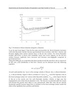
To illustrate the procedure of choosing collocation points let us consider an
inverse problem in a square (Hon & Wei, 2005):




12 1 2
,:0 1, 0 1xx x x



,




12 1 2
,: 1, 0 1
D
Sxxx x,




12 1 2
,:0 1, 1
N
Sxx x x

 ,


\
RDN
SSS  .
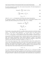
Distribution of the measurement points and collocation points is shown in Figure 1.
An approximation
T


to the solution of the inverse problem under the conditions (20)
2
, (20)
3

and (20)
6
and the noisy measurements
()k
i
Y

can be expressed by the following linear
combination:



1
, ,
nmpq
jjj
j
Tt tt





xxx


, (30)
where



,,*tFtt

xx, F is given by (29) and
j


are unknown coefficients to be
determined.
For this choice of basis functions

, the approximated solution T

automatically satisfies the
original heat equation (20)
1
. Using the conditions (20)
2
, (20)
3
and (20)
6 ,
we then obtain the
following system of linear equations for the unknown coefficients
j



:

Ab




(31)

Inverse Heat Conduction Problems

15

Fig. 1. Distribution of measurement points and collocation points. Stars represent collocation
points matching Dirichlet data, squares represent collocation points matching Neumann
data, dots represent collocation points matching initial data and circles denotes points with
sensors for internal measurement.
where




,
,
ijij
kjkj
tt
A
tt

n












xx
xx
(32)
and




1
2
,
,
,
i
ii
ii
kk

Y
ht
b
g
t
g
t








x
x
x


(33)
where


1,2, ,inm
p
,


1 , ,( )knm

p
mn
pq

   ,


1,2, ,
j
nm
pq

 ,
respectively. The first m rows of the matrix A leads to values of measurements, the next n
rows – to values of the right-hand side of the initial condition and, of course, time variable is
then equal to zero, the next p rows leads to values of the right-hand side of the Dirichlet
condition and the last q rows - to values of the right-hand side of Neumann condition.

Heat Conduction – Basic Research

16
The solvability of the system (31) depends on the non-singularity of the matrix A, which is
still an open research problem.
Fundamental solution method belongs to the family of Trefftz method. Both methods,
described in part 4.4 and 4.6, frequently lead to ill-conditioned system of algebraic equation.
To solve the system of equations, different techniques are used. Two of them, namely single
value decomposition and Tikhonov regularization technique, are briefly presented in the
further parts of the chapter.
4.7 Singular value decomposition
The ill-conditioning of the coefficient matrix A (formula (32) in the previous part of the

chapter) indicates that the numerical result is sensitive to the noise of the right hand side
b

(formula (33)) and the number of collocation points. In fact, the condition number of the
matrix A increases dramatically with respect to the total number of collocation points.
The singular value decomposition usually works well for the direct problems but usually
fails to provide a stable and accurate solution to the system (31). However, a number of
regularization methods have been developed for solving this kind of ill-conditioning
problem, (Hansen, 1992; Hansen & O’Leary, 1993). Therefore, it seems useful to present the
singular value decomposition method here.
Denote N = n + m + p + q. The singular value decomposition of the NN

matrix A is a
decomposition of the form

1

N
TT
iii
i
AWV


 

wv (34)
with



12
, , ,
N
W  ww w and


12
, , ,
N
V  vv v satisfying
TT
N
WW VV I. Here, the
superscript T denotes transposition of a matrix. It is known that


12
, , ,
N
diag
 
 has
non-negative diagonal elements satisfying inequality

12
0
N
 
 
(35)

The values
i

are called the singular values of A and the vectors
i
w and
i
v are called left
and right singular vectors of A, respectively, (Golub & Van Loan, 1998). The more rapid is
the decrease of singular values in (35), the less we can reconstruct reliably for a given noise
level. Equivalently, in order to get good reconstruction when the singular values decrease
rapidly, an extremely high signal-to-noise ratio in the data is required.
For the matrix A the singular values decay rapidly to zero and the ratio between the largest
and the smallest nonzero singular values is often huge. Based on the singular value
decomposition, it is easy to know that the solution for the system (31) is given by

1
T
N
i
i
i
i
b





w

v


(36)
When there are small singular values, such approach leads to a very bad reconstruction of
the vector


. It is better to consider small singular values as being effectively zero, and to
regard the components along such directions as being free parameters which are not
determined by the data.

Inverse Heat Conduction Problems

17
However, as it was stated above, the singular value decomposition usually fails for the
inverse problems. Therefore it is better to use here Tikhonov regularization method.
4.8 Tikhonov regularization method
This is perhaps the most common and well known of regularization schemes, (Tikhonov &
Arsenin, 1977). Instead of looking directly for a solution for an ill-posed problem (31) we
consider a minimum of a functional

2
2
2
0
JAb




 


 
(37)
with
0


being a known vector,
. denotes the Euclidean norm, and
2

is called the
regularization parameter. The necessary condition of minimum of the functional (37) leads
to the following system of equation:




2
0
0
T
AA b






.
Hence




1
22
0
TT
AA I Ab



 



Taking into account (34) after transformation one obtains the following form of the
functional
J:





2
2
2
0

2
2
2
2
22
00
TT T
JWVWWb VV
WV J
 


   

    yc yy yc yy y

 
(38)
where
T
V

y

,
0
T
V

y


,
T
Wbc

and the use has been made from the properties
TT
N
WW VV I. Minimization of the functional


J y leads to the following vector
equation:




2
0
0
T


   yc yy or


22
0
TT


   yy cy
.
Hence

2
0
22 22
i
ii i
ii
y
c
y


 


, 1, ,iN

or
2
0
22 22
1
N
T
i
ii
i

ii
b




 








wv


(39)
If
0

 0

the Tikhonov regularized solution for equation (31) based on singular value
decomposition of the
NN

matrix A can be expressed as

22
1
N
T
i
ii
i
i
b








wv


(40)

Heat Conduction – Basic Research

18
The determination of a suitable value of the regularization parameter
2

is crucial and is
still under intensive research. Recently the L-curve criterion is frequently used to choose a

good regularization parameter, (Hansen, 1992; Hansen & O’Leary, 1993). Define a curve L
by



2
2
log ,logLAb
















(41)
A suitable regularization parameter
2

is the one near the “corner” of the L-curve, (Hansen
& O’Leary, 1993; Hansen, 2000).

4.9 The conjugate gradient method
The conjugate gradient method is a straightforward and powerful iterative technique for
solving linear and nonlinear inverse problems of parameter estimation. In the iterative
procedure, at each iteration a suitable step size is taken along a direction of descent in order
to minimize the objective function. The direction of descent is obtained as a linear
combination of the negative gradient direction at the current iteration with the direction of
descent of the previous iteration. The linear combination is such that the resulting angle
between the direction of descent and the negative gradient direction is less than 90
o
and the
minimization of the objective function is assured, (Özisik & Orlande, 2000).
As an example consider the following problem in a flat slab with the unknown heat source


p
gt in the middle plane:




22
/0.5/
p
Txgtx Tt


    in 0 1x

 , for 0t 

/0
Tx


at 0x

and at 1x

, for 0t  (42)


,0 0Tx

for 0t

, in 0 1x


where



 is the Dirac delta function. Application of the conjugate gradient method can be
organized in the following steps (Özisik & Orlande, 2000):
 The direct problem,
 The inverse problem,
 The iterative procedure,
 The stopping criterion,
 The computational algorithm.
The direct problem. In the direct problem associated with the problem (42) the source

strength,


p
gt
, is known. Solving the direct problem one determines the transient
temperature field


,Txt in the slab.
The inverse problem. For solution of the inverse problem we consider the unknown energy
generation function


p
gt
to be parameterized in the following form of linear combination
of trial functions


j
Ct
(e.g. polynomials, B-splines, etc.):

Inverse Heat Conduction Problems

19

 
1

N
pjj
j
gt PCt



(43)
j
P
are unknown parameters, 1,2, ,jN

. The total number of parameters, N, is specified.
The solution of the inverse problem is based on minimization of the ordinary least square
norm,


S P :

   
2
1
I
T
ii
i
SYT


   


  

PPYTPYTP (44)
where


12
, , ,
T
N
PP PP
,




,
ii
TTtPP states for estimated temperature at time
i
t ,


ii
YYt
denotes measured temperature at time
i
t , I is a total number of measurements,
IN . The parameters estimation problem is solved by minimization of the norm (44).

The iterative procedure. The iterative procedure for the minimization of the norm S(P) is
given by

1kkkk


PP d (45)
where
k

is the search step size,
12
, , ,
kkkk
N
dd d





d
is the direction of descent and k is the
number of iteration.
k
d is a conjugation of the gradient direction,


k
S P , and the direction

of descent of the previous iteration,
1k

d :



1kkkk
S


 dPd. (46)
Different expressions are available for the conjugation coefficient
k

. For instance the
Fletcher-Reeves expression is given as



2
1
2
1
1
N
k
j
j
k

N
k
j
j
S
S

















P
P
for 1,2, k

with
0
0



. (47)
Here

 
1
2
k
I
kk
i
ii
j
j
i
T
SYT
P




 




PP for 1,2, ,jN . (48)
Note that if 0

k

 for all iterations k, the direction of descent becomes the gradient direction
in (46) and the steepest-descent method is obtained.
The search step
k

is obtained by minimizing the function


1k
S

P
with respect to
k

. It
yields the following expression for
k

:

Heat Conduction – Basic Research

20


1
2

1
T
I
kk
i
ii
k
i
k
T
I
k
i
k
i
T
TY
T






























dP
P
d
P
, where
12
, , ,
T
iiii
kkkk
N
TTTT
PP P















P
. (49)
The stopping criterion. The iterative procedure does not provide the conjugate gradient
method with the stabilization necessary for the minimization of


S P
to be classified as
well-posed. Such is the case because of the random errors inherent to the measured
temperatures. However, the method may become well-posed if the Discrepancy Principle is
used to stop the iterative procedure, (Alifanov, 1994):



1k
S




P (50)
where the value of the tolerance ε is chosen so that sufficiently stable solutions are obtained,
i.e. when the residuals between measured and estimated temperatures are of the same order
of magnitude of measurement errors, that is




,
imeasii
Yt Tx t



, where
i

is the
standard deviation of the measurement error at time t
i
. For
i
const



 we obtain I



 .
Such a procedure gives the conjugate gradient method an iterative regularization character. If
the measurements are regarded as errorless, the tolerance ε can be chosen as a sufficiently
small number, since the expected minimum value for the


S P
is zero.
The computation algorithm. Suppose that temperature measurements


12
, , ,
I
YY YY are
given at times t
i
, 1,2, ,iI

, and an initial guess
0
P is available for the vector of unknown
parameters
P. Set k = 0 and then
Step 1. Solve the direct heat transfer problem (42) by using the available estimate
k
P and
obtain the vector of estimated temperatures




12
, , ,
k
I
TT TTP .
Step 2. Check the stopping criterion given by equation (50). Continue if not satisfied.
Step 3. Compute the gradient direction


k
S P from equation (48) and then the conjugation
coefficient
k

from (47).
Step 4. Compute the direction of descent
k
d by using equation (46).
Step 5. Compute the search step size
k

from formula (49).
Step 6. Compute the new estimate
1k

P using (45).
Step 7. Replace k

by k+l and return to step 1.
4.10 The Levenberg-Marquardt method
The Levenberg-Marquardt method, originally devised for application to nonlinear
parameter estimation problems, has also been successfully applied to the solution of linear
ill-conditioned problems. Application of the method can be organized as for conjugate
gradient. As an example we will again consider the problem (42).
The first two steps,
the direct problem and the inverse problem, are the same as for
the conjugate gradient method.

Inverse Heat Conduction Problems

21
The iterative procedure. To minimize the least squares norm, (44), we need to equate to
zero the derivatives of S(P) with respect to each of the unknown parameters


12
, , ,
N
PP P ,that is,







12
0

N
SS S
PP P
 

 
 
PP P
(51)
Let us introduce the Sensitivity or Jacobian matrix, as follows:



11 1
12
22 2
12
12
N
T
T
N
II I
N
TT T
PP P
TT T
PP P
TT T
PP P

 




 




 




 











 





 


TP
JP
P
or
i
ij
j
T
J
P



(52)
where N = total number of unknown parameters, I= total number of measurements. The
elements of the sensitivity matrix are called the sensitivity coefficients
, (Özisik & Orlande,
2000). The results of differentiation (51) can be written down as follows:

 
20
T

 


JPYTP
(53)
For linear inverse problem the sensitivity matrix is not a function of the unknown
parameters. The equation (53) can be solved then in explicit form (Beck & Arnold, 1977):



1
TT

PJJJY (54)
In the case of a nonlinear inverse problem, the matrix
J has some functional dependence on the
vector
P. The solution of equation (53) requires then an iterative procedure, which is
obtained by linearizing the vector
T(P) with a Taylor series expansion around the current
solution at iteration k. Such a linearization is given by






kk k
TP TP J P P
(55)
where



k
TP and
k
J
are the estimated temperatures and the sensitivity matrix evaluated at
iteration k, respectively. Equation (55) is substituted into (54) and the resulting expression is
rearranged to yield the following iterative procedure to obtain the vector of unknown
parameters
P (Beck & Arnold, 1977):

11
[( ) ] ( ) [ ( )]
kkkTkkT k
 PPJJJYTP
(56)
The iterative procedure given by equation (56) is called the Gauss method. Such method is
actually an approximation for the Newton (or Newton-Raphson) method. We note that

Heat Conduction – Basic Research

22
equation (54), as well as the implementation of the iterative procedure given by equation
(56), require the matrix
T
J
J to be nonsingular, or

0
T


JJ (57)
where
. is the determinant.
Formula (57) gives the so called Identifiability Condition, that is, if the determinant of
T
J
J is
zero, or even very small, the parameters P
j
, for 1,2, ,jN

, cannot be determined by
using the iterative procedure of equation (56).
Problems satisfying
T

J
J 0 are denoted ill-conditioned. Inverse heat transfer problems are
generally very ill-conditioned, especially near the initial guess used for the unknown
parameters, creating difficulties in the application of equations (54) or (56). The Levenberg-
Marquardt method alleviates such difficulties by utilizing an iterative procedure in the
form, (Özisik & Orlande, 2000):

11
[( ) ] ( ) [ ( )]
kkkTkkkkT k


  PPJJ JYTP (58)
where

k

is a positive scalar named damping parameter and
k

is a diagonal matrix.
The purpose of the matrix term
kk


is to damp oscillations and instabilities due to the ill-
conditioned character of the problem, by making its components large as compared to those
of
T
J
J if necessary.
k

is made large in the beginning of the iterations, since the problem is
generally ill-conditioned in the region around the initial guess used for iterative procedure,
which can be quite far from the exact parameters. With such an approach, the matrix
T
J
J is
not required to be non-singular in the beginning of iterations and the Levenberg-Marquardt
method tends to the steepest descent method, that is , a very small step is taken in the negative
gradient direction. The parameter
k

is then gradually reduced as the iteration procedure

advances to the solution of the parameter estimation problem, and then the Levenberg-
Marquardt method tends to the Gauss method given by (56).
The stopping criteria. The following criteria were suggested in (Dennis & Schnabel, 1983) to
stop the iterative procedure of the Levenberg-Marquardt Method given by equation (58):


1
1
k
S



P




2
[()]
kk


JYTP (59)
1
3
kk


PP

where
1

,
2

and
3

are user prescribed tolerances and . denotes the Euclidean norm.

The computational algorithm. Different versions of the Levenberg-Marquardt method can be
found in the literature, depending on the choice of the diagonal matrix d and on the form
chosen for the variation of the damping parameter

k
(Özisik & Orlande, 2000). [l-91. Here

Inverse Heat Conduction Problems

23

[( ) ]
kkTk
diag JJ
. (60)
Suppose that temperature measurements


12

, , ,
I
YY YY
are given at times t
i
, 1,2, ,iI ,
and an initial guess

0
P
is available for the vector of unknown parameters P. Choose a value
for
0

, say,
0

= 0.001 and set k=0. Then,
Step 1. Solve the direct heat transfer problem (42) with the available estimate
k
P in order to
obtain the vector



12
, , ,
k
I
TT TTP .

Step 2. Compute ( )
k
S P from the equation (44).
Step 3. Compute the sensitivity matrix
k
J
from (52) and then the matrix
k

from (60), by
using the current value of
k
P .
Step 4. Solve the following linear system of algebraic equations, obtained from (58):

[( ) ] ( ) [ ( )]
kT k k k k kT k

 JJ P J YTP
(61)
in order to compute
1kk k

PP P.
Step 5. Compute the new estimate
1k

P as

1kkk


PPP (62)
Step 6. Solve the
exact problem (42) with the new estimate
1k

P in order to find

1k
TP .
Then compute
1
()
k
S

P .
Step 7. If
1
()()
kk
SS

PP
, replace
k

by 10
k


and return to step 4.
Step 8. If
1
()()
kk
SS

PP, accept the new estimate
1k

P and eplace
k

by 0,1
k

.
Step 9. Check the stopping criteria given by (59). Stop the iterative procedure if any of them
is satisfied; otherwise, replace k by k+1 and return to step 3.
4.11 Kalman filter method
Inverse problems can be regarded as a case of system identification problems. System
identification has enjoyed outstanding attention as a research subject. Among a variety of
methods successfully applied to them, the Kalman filter, (Kalman, 1960; Norton,
1986;Kurpisz. & Nowak, 1995), is particularly suitable for inverse problems.
The Kalman filter is a set of mathematical equations that provides an efficient computational
(recursive) solution of the least-squares method. The Kalman filtering technique has been
chosen extensively as a tool to solve the parameter estimation problem. The technique is
simple and efficient, takes explicit measurement uncertainty incrementally (recursively),
and can also take into account a priori information, if any.
The Kalman filter estimates a process by using a form of feedback control. To be precise, it

estimates the process state at some time and then obtains feedback in the form of noisy
measurements. As such, the equations for the Kalman filter fall into two categories: time
update and measurement update equations. The time update equations project forward (in
time) the current state and error covariance estimates to obtain the a priori estimates for the
next time step. The measurement update equations are responsible for the feedback by

Heat Conduction – Basic Research

24
incorporating a new measurement into the a priori estimate to obtain an improved a posteriori
estimate. The time update equations are thus predictor equations while the measurement
update equations are corrector equations.
The standard Kalman filter addresses the general problem of trying to estimate x
∈ℜ of a
dynamic system governed by a linear stochastic difference equation, (Neaupane &
Sugimoto, 2003)
4.12 Finite element method
The finite element method (FEM) or finite element analysis (FEA) is based on the idea of
dividing the complicated object into small and manageable pieces. For example a two-
dimensional domain can be divided and approximated by a set of triangles or rectangles (the
elements or cells). On each element the function is approximated by a characteristic form.
The theory of FEM is well know and described in many monographs, e.g. (Zienkiewicz,
1977; Reddy & Gartling, 2001). The classic FEM ensures continuity of an approximate
solution on the neighbouring elements. The solution in an element is built in the form of
linear combination of shape function. The shape functions in general do not satisfy the
differential equation which describes the considered problem. Therefore, when used to solve
approximately an inverse heat transfer problem, usually leads to not satisfactory results.
The FEM leads to promising results when T-functions (see part 4.4) are used as shape
functions. Application of the T-functions as base functions of FEM to solving the inverse
heat conduction problem was reported in (Ciałkowski, 2001). A functional leading to the

Finite Element Method with Trefftz functions may have other interpretation than usually
accepted. Usually the functional describes mean-square fitting of the approximated
temperature field to the initial and boundary conditions. For heat conduction equation the
functional is interpreted as mean-square sum of defects in heat flux flowing from element to
element, with condition of continuity of temperature in the common nodes of elements. Full
continuity between elements is not ensured because of finite number of base functions in
each element.
However, even the condition of temperature continuity in nodes may be weakened. Three
different versions of the FEM with T-functions (FEMT) are considered in solving inverse
heat conduction problems: (a) FEMT with the condition of continuity of temperature in the
common nodes of elements, (b) no temperature continuity at any point between elements
and (c) nodeless FEMT.
Let us discuss the three approaches on an example of a dimensionless 2D transient
boundary inverse problem in a square


(,):0 1, 0 1xy x y

, for t > 0. Assume that
for
0y 
the boundary condition is not known; instead measured values of temperature,
ik
Y
, are known at points


1,,
bik
y

t

 . Furthermore,




0
0
,, ,
t
Txyt T xy

 ,
1
0
(,,) (,)
x
Txyt h yt


,
2
1
(,,) (,)
y
T
xyt h xt
y





,

3
0
(,,) (,)
y
T
xyt h xt
y




(63)

Inverse Heat Conduction Problems

25
(a) FEMT with the condition of continuity of temperature in the common nodes of elements
(Figure 2). We consider time-space finite elements. The approximate temperature in a j-th
element,

,,
j
Txyt

, is a linear combination of the T-functions, (,,)

m
Vxyt:




1
(,,) ,, (,,) (,,)
N
T
jj j
mm
m
T xyt T xyt cV xyt C Vxyt

 


(64)
where N is the number of nodes in the j-th element and [V(x, y, t)] is the column matrix
consisting of the T-functions. The continuity of the solution in the nodes leads to the
following matrix equation in the element:



[][]VC T (65)
In (65) elements of matrix
[]V stand for values of the T-functions, (,,)
m
Vxyt, in the

nodal points, i.e.


,,
rs
srrr
VVxyt , r,s = 1,2,…,N. The column matrix
12
[] [ , , , ]
jj
N
j
T
TTT T consists of temperatures (mostly unknown) of the nodal points with
i
j
T standing for value of temperature in the i-th node, i = 1,2,…,N. The unknown
coefficients of the linear combination (63) are the elements of the column matrix [C]. Hence
we obtain





1
[]CVT

 and finally



1
( , , ) ([ ] [ ]) [ , , ]
j
T
T xyt V T V xyt



(66)
It is clear, that in each element the temperature
(,,)
j
Txyt

satisfies the heat conduction
equation. The elements of matrix
1
([ ] [ ])
T
VT

can be calculated from minimization of the
objective functional, describing the mean-square fitting of the approximated temperature
field to the initial and boundary conditions.


Fig. 2. Time-space elements in the case of temperature continuous in the nodes.
(b) No temperature continuity at any point between elements (Figure 3). The approximate
temperature in a j-th element,



,,
j
Txyt

, is a linear combination of the T-functions (63),
too. In this case in order to ensure the physical sense of the solution we minimize
inaccuracy of the temperature on the borders between elements. It means that the
functional describing the mean-square fitting of the approximated temperature field to

Heat Conduction – Basic Research

26
the initial and boundary conditions includes the temperature jump on the borders
between elements. For the case





 



,
22
01
0
22
23

00
2
2
,1
0
1
,,0 (,) 0,, ,
,1, , ,0, ,
,,
e
ii
ee
ii
e
ITR
ij
b
t
ii
ii
tt
ii
ii
t
I
ij ikkk ik
ij i k
x
JTxyTxyddtTythytd
TT

dt x t h x t d dt x t h x t d
yy
dt T T d T x y t Y






 


 



 



 




 
(67)


Fig. 3. Time-space elements in the case of temperature discontinuous in the nodes.

(c) Nodeless FEMT. Again,


,,
j
Txyt

, is a linear combination of the T-functions. The time
interval is divided into subintervals. In each subinterval the domain  is divided into J
subdomains (finite elements) and in each subdomain 
j
, j=1, 2,…, J (with
ii
) the
temperature is approximated with the linear combination of the Trefftz functions according
to the formula (64). The dimensionless time belongs to the considered subinterval. In the
case of the first subinterval an initial condition is known. For the next subintervals initial
condition is understood as the temperature distribution in the subdomain 
j
at the final
moment of time in the previous subinterval. The mean-square method is used to minimize
the inaccuracy of the approximate solution on the boundary, at the initial moment of time
and on the borders between elements. This way the unknown coefficients of the
combination,
j
m
c , can be calculated. Generally, the coefficients
j
m
c depend on the time

subinterval number, (Grysa & Lesniewska, 2009).
In (Ciałkowski et al., 2007) the FEM with Trefftz base functions (FEMT) has been compared
with the classic FEM approach. The FEM solution of the inverse problem for the square
considered was analysed. For the FEM the elements with four nodes and, consequently, the
simplest set of base functions:
(1, , , )xyxyhave been applied.
Consider an inverse problem in a square (compare the paragraph before the equation (63)).
Using FEM to solve the inverse problem gives acceptable solution only for the first row of
elements. Even for exact values of the given temperature the results are encumbered with

Inverse Heat Conduction Problems

27
relatively high error. For the next row of the elements, the FEM solution is entirely not
acceptable. When the distance
b

greater than the size of the element, an instability of the
numerical solution appears independently of the number of finite elements. Paradoxically,
the greater number of elements, the sooner the instability appears even though the accuracy
of solution in the first row of elements becomes better. The classic FEM leads to much worse
results than the FEMT because the latter makes use of the Trefftz functions which satisfy the
energy equation. This way the physical meaning of the results is ensured.
4.13 Energetic regularization in FEM
Three kinds of physical aspects of heat conduction can be applied to regularize an
approximate solution obtained with the use of finite element method, (Ciałkowski et al.,
2007). The first is minimization of heat flux jump between the elements, the second is
minimization of the defect of energy dissipation on the border between elements and the
third is the minimization of the intensity of entropy production between elements. Three
kinds of regularizing terms for the objective functional are proposed:

-
minimizing the heat flux inaccuracy between elements:

,
2
,
0
e
ij
t
j
i
ij
ij
T
T
dt d
nn















(68)
-
minimizing numerical entropy production between elements:

,
2
,
0
11
e
ij
t
j
i
ij
ij
ij
T
T
dt d
nn
TT
















, and (69)
-
minimizing the defect of energy of dissipation between elements:

,
2
,
0
ln ln
e
ij
t
j
i
ij
ij
ij
T
T
dt T T d
nn
















(70)
with t
f
being the final moment of the considered time interval, (Ciałkowski et al., 2007; Grysa
& Leśniewska, 2009), and
,i
j

standing for the border between i-th and j-th element.
Notice that entropy production functional and energy dissipation functional are not
quadratic functions of the coefficients of the base functions in elements. Hence, minimizing
the objective functional leads to a non-linear system of algebraic equations. It seems to be
the only disadvantage when compared with minimizing mean-square defects of heat flux
(formula (68)); the latter leads to a system of linear equations.
4.14 Other methods

Many other methods are used to solve the inverse heat conduction problems. Many iterative
methods for approximate solution of inverse problems are presented in monograph
(Bakushinsky & Kokurin, 2004). Numerical methods for solving inverse problems of
mathematical physics are presented in monograph (Samarski & Vabishchevich, 2007). Among
other methods it is worth to mention boundary element method (Białecki et al., 2006; Onyango

Heat Conduction – Basic Research

28
et al., 2008), the finite difference method (Luo & Shih, 2005; Soti et al., 2007), the theory of
potentials method (Grysa, 1989), the radial basis functions method (Kołodziej et al., 2010), the
artificial bee colony method (Hetmaniok et al., 2010), the Alifanov iterative regularization
(Alifanov, 1994), the optimal dynamic filtration, (Guzik & Styrylska, 2002), the control volume
approach (Taler & Zima, 1999), the meshless methods ((Sladek et al., 2006) and many other.
5. Examples of the inverse heat conduction problems
5.1 Inverse problems for the cooled gas turbine blade
Let us consider the following stationary problem concerning the gas turbine blade (Figure
4): find temperature distribution on the
inner boundary
i

of the blade cross-section,
i
T

,
and heat transfer coefficient variation along
i

, with the condition



00TT
TTsT



 (71)
where
T

stands for temperature measurement tolerance and s is a normalized coordinate
of a perimeter length (black dots in Figure 4 denote the beginning and the end of the inner
and outer perimeter, coordinate is counted counterclockwise). Heat transfer coefficient
distribution at the outer surface,
o
c
h

, is known, T
fo
= 1350
o
C, T
fi
=780oC, T
0
= 1100
o

C ,
T

,
standing for temperature measurement tolerance, does not exceed 1
o
C. Moreover, the inner
and outer fluid temperature T
fo
and T
fi
are known, (Ciałkowski et al., 2007a). The
unknowns
: ?
i
T

 , ?
i
c
h


The solution has to be found in the class of functions fulfilling
the energy equation



0kT



(72)


Fig. 4. An outline of a turbine blade.
with k assumed to be a constant. To solve the problem we use FEM with the shape functions
belonging to the class of harmonic functions. It means that we can express an approximate

Inverse Heat Conduction Problems

29
solution of a stationary heat conduction problem in each element as a linear combination of
the T-functions suitable for the equation (72). The functional with a term minimizing the
heat flux inaccuracy between elements reads



,,
2
2
()
ij ij
ij
IT q q d w T T d

 







 






with
T
qk
n



(73)
In order to simplify the problem, temperature on the outer and inner surfaces was then
approximated with 5 and 30 Bernstein polynomials, respectively, in order to simplify the
problem. The area of the blade cross-section was divided into 99 rectangular finite elements
with 16 nodes (12 on the boundary of each element and 4 inside). 16 harmonic (Trefftz)
functions were used as base functions. All together 4x297 unknowns were introduced.
Calculations were carried out with the use of PC with
1.6 GHz processor. Time of
calculation was 1,5 hours using authors’ own computer program in Fortran F90. The results
are presented at Figures 5 and 6.



Fig. 5. Temperature [

o
C] (upper) and heat flux (lower) distribution on the outer (red squares)
and inner (dark blue dots) surfaces of the blade.

Heat Conduction – Basic Research

30
Oscillations of temperature of the inner blade surface (Figure 5 left) is due to the number
of Bernstein polynomials: it was too small. However, thanks to a small number of the
polynomials a small number of unknown values of temperature could be taken for
calculation. The same phenomenon appears in Figure 5 right for heat flux on the inner
blade surface as well as in Figure 6 for the heat transfer coefficients values. The distance
between peaks of the curves for the inner and outer surfaces in Figure 6 is a result of
coordinate normalization of the inner and outer surfaces perimeter length. The
normalization was done in such a way that only for s = 0 (s =1) points on both surfaces
correspond to each other. The other points with the same value of the coordinate s for the
outer and inner surface generally do not correspond to each other (in the case of peaks the
difference is about 0,02).


Fig. 6
. Heat transfer coefficient over inner (dark blue squares) and outer (red dots — given;
brown dots — calculated) surfaces of the blade.
5.2 Direct solution of a heat transfer coefficient identification problem
Consider a 1D dimensionless problem of heat conduction in a thermally isotropic flat slab
(Grysa, 1982):

22
//Tx Tt


  for (0,1)x

and t(0, t
f
],

Inverse Heat Conduction Problems

31
/0Tx

 for x = 0 and t(0, t
f
], (74)

 
/1,
f
kT x BiT t T t


 


for x = 1 and t(0, t
f
],
0T

for (0,1)x


and t = 0 .
If the upper surface temperature (for x = 1) cannot be measured directly then in order to find
the Biot number, temperature responses at some inner points of the slab or even
temperature of the lower surface (x = 0) have to be known. Hence, the problem is ill-posed.
Employing the Laplace transformation to the problem (74) we obtain
 
cosh
,
sinh cosh
f
Bi x s
Txs T s
ssBis


or

  
cosh 1 1 sinh
,,
cosh cosh
f
xs s
Ts Txs Txs
sBi
ss ss

(75)
The equation (75) is then used to find the formula describing the Biot number, Bi. Then, the

inverse Laplace transformation yields:







  
2
1
2
1
2, exp
1
12 cos exp ,
n
n
n
fnn
n
n
Tx t
Bi
Tt x t Ht xt

 











   




(76)
Here asterisk denotes convolution,


H

is the Heaviside function and

21/2
n
n

,
n = 1,2,… .
If the temperature is known on the boundary x = 0 (e.g. from measurements), values of Bi
(because of noisy input data having form of a function of time) can be calculated from
formula (76). Of course, formula (76) is obtained with the assumption that Bi = const.
Therefore, the results have to be averaged in the considered time interval.

6. Final remarks
It is not possible to present such a broad topic like inverse heat conduction problems in one
short chapter. Many interesting achievements were discussed very briefly, some were
omitted. Little attention was paid to stochastic methods. Also, the non-linear issues were
only mentioned when discussing some methods of solving inverse problems. For lack of
space only few examples could be presented.
The inverse heat conduction problems have been presented in many monographs and
tutorials. Some of them are mentioned in references, e.g. (Alifanov, 1994; Bakushinsky &
Kokurin, 2004; Beck & Arnold, 1977; Grysa, 2010; Kurpisz & Nowak, 1995; Özisik &
Orlande, 2000; Samarski & Vabishchevich, 2007; Duda & Taler, 2006; Hohage, 2002; Bal,
2004; Tan & Fox, 2009).

Heat Conduction – Basic Research

32
7. References
Alifanov, O. M. (1994), Inverse heat transfer problems, Springer-Verlag, ISBN 0-387-53679-5,
New York
Anderssen, R. S. (2005), Inverse problems: A pragmatist’s approach to the recovery of
information from indirect measurements, Australian and New Zealand Industrial and
Applied Mathematics Journal Vol.46, pp. C588 C622, ISSN 1445-8735
Bakushinsky, A. B. & Kokurin M. Yu. (2004), Iterative Methods for Approximate Solution of
Inverse Problems, Springer, ISBN 1-4020-3121-1, Dordrecht, The Netherlands
Bal. G, (2004), Lecture Notes, Introduction to Inverse Problems, Columbia University, New York,
Date of acces: June 30, 2011, Available from:

Beck, J. V. & Arnold, K. J. (1977) Parameter Estimation in Engineering and Science, Wiley, ISBN
0471061182, New York
Beck, J. V. (1962), Calculation of surface heat flux from an internal temperature history,
ASME Paper 62-HT-46

Beck, J. V., Blackwell B. & St. Clair, Jr, R. St. (1985), Inverse heat conduction, A Wiley-
Interscience Publication, ISBN 0-471-08319-4, New York – Chichester – Brisbane –
Toronto – Singapure
Bialecki, R., Divo E. & Kassab, A. (2006), Reconstruction of time-dependent boundary heat
flux by a BEM-based inverse algorithm, Engineering Analysis with Boundary
Elements, Vol.30, No.9, September 2006, pp. 767-773, ISSN 0955-7997
Burggraf, O. R. (1964), An Exact Solution of the Inverse Problem in Heat Conduction Theory
and Application, Journal of Heat Transfer, Vol.86, August 1964, pp.373-382,
ISSN 0022-1481
Chen, C. S., Karageorghis, A. & Smyrlis Y.S. (2008), The Method of Fundamental Solutions – A
Meshless Method, Dynamic Publishers, Inc., ISBN 1890888-04-4, Atlanta, USA
Cheng, C.H. & Chang, M.H. (2003), Shape design for a cylinder with uniform temperature
distribution on the outer surface by inverse heat transfer method, International
Journal of Heat and Mass Transfer, Vol.46, No.1, (January 2003), pp. 101-111,
ISSN 0017-9310
Ciałkowski, M. J. (2001), New type of basic functions of FEM in application to solution of
inverse heat conduction problem, Journal of Thermal Science, Vol.11, No.2, pp. 163–
171, ISSN 1003-2169
Ciałkowski, M. J., Frąckowiak, A. & Grysa, K. (2007), Solution of a stationary inverse
heat conduction problem by means of Trefftz non-continuous method,
International Journal of Heat and Mass Transfer Vol.50, No.11-12, pp.2170–2181,
ISSN 0017-9310
Cialkowski, M. J., Frąckowiak, A. & Grysa, K. (2007a), Physical regularization for inverse
problems of stationary heat conduction, Journal of Inverse and Ill-Posed Problems,
Vol.15, No.4, pp. 347–364. ISSN 0928-0219
Ciałkowski, M. J. & Grysa, K. (2010), A sequential and global method of solving an inverse
problem of heat conduction equation, Journal of Theoretical and Applied Mechanics,
Vol.48, No.1, pp. 111-134, ISSN 1429-2955

Inverse Heat Conduction Problems

33
Ciałkowski, M. J. & Grysa, K. (2010a), Trefftz method in solving the inverse problems,
Journal of Inverse and Ill-posed Problems, Vol.18, No.6, pp. 595
–616, ISSN 0928-
0219
Dennis, B. H., Dulikravich, G. S. Egorov, I. N., Yoshimura, S. & Herceg, D. (2009), Three-
Dimensional Parametric Shape Optimization Using Parallel Computers,
Computational Fluid Dynamics Journal, Vol.17, No.4, pp.256–266, ISSN 0918-6654
Dennis, J. & Schnabel, R. (1983), Numerical Methods for Unconstrained Optimization and
Nonlinear Equations, Prentice Hall, ISBN 0-89871-364-1
Duda, P. & Taler, J. (2006), Solving Direct and Inverse Heat Conduction Problems, Springer,
ISBN 354033470X
Fan, Y. & Li, D G. (2009), Identifying the Heat Source for the Heat Equation with
Convection Term, International Journal of Mathematical Analysis, Vol.3, No.27, pp.
1317–1323, ISSN 1312-8876
Golub, G. & Van Loan, C.(1998), Matrix Computations.: The Johns Hopkins University Press,
ISBN 0-8018-5413-X, Baltimore, USA
Guzik, A. & Styrylska, T (2002), An application of the generalized optimal dynamic filtration
method for solving inverse heat transfer problems, Numerical Heat Transfer, Vol.42,
No.5, October 2002, pp.531-548, ISSN 1040-7782
Grysa, K. (1982), Methods of determination of the Biot number and the heat transfer
coefficient, Journal of Theoretical and Applied Mechanics, 20, 1/2, 71-86, ISSN 1429-
2955
Grysa, K. (1989), On the exact and approximate methods of solving inverse problems of temperature
fields, Rozprawy 204, Politechnika Poznańska, ISBN 0551-6528, Poznań, Poland
Grysa, K. & Lesniewska, R. (2009), Different Finite Element Approaches For The Inverse
Heat Conduction Problems, Inverse Problems in Science and Engineering, Vol.18, No.1
pp. 3-17, ISSN 1741-5977
Grysa, K. & Maciejewska, B. (2005), Application of the modified finite elements method to

identify a moving heat source, In: Numerical Heat Transfer 2005, Vol.2, pp. 493-502,
ISBN 83-922381-2-5, EUTOTERM 82, Gliwice-Cracow, Poland, September 13-16,
2005
Grysa, K. (2010), Trefftz functions and their Applications in Solving Inverse Problems,
Politechnika Świętokrzyska, PL ISSN 1897-2691, (in Polish)
Hadamard, J. (1923), Lectures on the Cauchy's Problem in Linear Partial Differential Equations,
Yale University Press, New Haven, recent edition: Nabu Press, 2010,
ISBN 9781177646918
Hansen, P. C. (1992), Analysis of discrete ill-posed problems by means of the L-curve, SIAM
Review, Vol.34, No.4, pp. 561–580, ISSN 0036-1445
Hansen, P. C. (2000), The L-curve and its use in the numerical treatment of inverse
problems, In: Computational Inverse Problems in Electrocardiology, P. Johnston (Ed.),
119-142, Advances in Computational Bioengineering. Available, WIT Press, from

Hansen, P.C. & O’Leary, D.P. (1993), The use of the L-curve in the regularization of discrete
ill-posed problems, SIAM Journal of Scientific Computing, Vol.14, No.6, pp. 1487–
1503, ISSN
1064-8275

Heat Conduction – Basic Research

34
Hetmaniok, E., Słota, D. & Zielonka A. (2010), Solution of the inverse heat conduction
problem by using the ABC algorithm, Proceedings of the 7th international conference on
Rough sets and current trends in computing RSCTC'10, pp.659-668, ISBN:3-642-13528-
5, Springer-Verlag, Berlin, Heidelberg
Hohage, T. (2002), Lecture Notes on Inverse Problems, University of Goettingen. Date of acces :
June 30, 2011, Available from
/>Kaltenbacher-WS0607/ip.pdf
Hon, Y.C. & Wei, T. (2005), The method of fundamental solutions for solving

multidimensional inverse heat conduction problems, Computer Modeling in
Engineering & Sciences, Vol.7, No.2, pp. 119-132, ISSN 1526-1492
Hożejowski, L., Grysa, K., Marczewski, W. & Sendek-Matysiak, E. (2009), Thermal
diffusivity estimation from temperature measurements with a use of a thermal
probe, Proceedings of the International Conference Experimental Fluid Mechanics 2009,
pp. 63-72, ISBN 978-80-7372-538-9, Liberec, Czech Republic, November 25 27,
2009
Ikehata, M. (2007), An inverse source problem for the heat equation and the enclosure
method, Inverse Problems, Vol. 23, No 1, pp. 183–202, ISSN 0266-5611
Jin, B. & Marin, L. (2007), The method of fundamental solutions for inverse source problems
associated with the steady-state heat conduction, International Journal for Numerical
Methods in Engineering, Vol.69, No.8, pp. 1570–1589, ISSN 0029-5981
Kalman, R. E. (1960), A New Approach to Linear Filtering and Prediction Problems,
Transactions of the ASME – Journal of Basic Engineering, Vol.82, pp. 35-45, ISSN 0021-
9223
Kołodziej, J. A., Mierzwiczak, M. & Ciałkowski M. J. (2010), Application of the method of
fundamental solutions and radial basis functions for inverse heat source problem in
case of steady-state, International Communications in Heat and Mass Transfer, Vol.37,
No.2, February 2010, pp.121-124, ISSN 0735-1933
Kover'yanov, A. V. (1967), Inverse problem of nonsteady state thermal conductivity,
Teplofizika vysokikh temperatur, Vol.5 No.1, pp.141-148, ISSN 0040-3644
Kurpisz, K. & Nowak, A. J. (1995), Inverse Thermal Problems, Computational Mechanics
Publications, ISBN 1 85312 276 9, Southampton, UK
Lorentz, G. G. (1953), Bernstein Polynomials. University of Toronto Press, ISBN 0-8284-0323-
6, Toronto,
Luo, J. & Shih, A. J. (2005), Inverse Heat Transfer Solution of the Heat Flux Due to Induction
Heating, Journal of Manufacturing Science and Engineering, Vol.127, No.3, pp.555-563,
ISSN 1087-1357
Masood, K., Messaoudi, S. & Zaman, F.D. (2002), Initial inverse problem in heat equation
with Bessel operator, International Journal of Heat and Mass Transfer, Vol.45, No.14,

pp. 2959–2965, ISSN 0017-9310
Monde, M., Arima, H., Liu, W., Mitutake, Y. & Hammad, J.A. (2003), An analytical solution
for two-dimensional inverse heat conduction problems using Laplace transform,
International Journal of Heat and Mass Transfer, Vol.46, No.12, pp. 2135–2148, ISSN
0017-9310

Inverse Heat Conduction Problems

35
Neaupane, K. M. & Sugimoto, M. (2003), An inverse Boundary Value problem using the
Extended Kalman Filter, ScienceAsia, Vol.29, pp.121-126, ISSN 1513-1874
Norton, J. P. (1986), An Introduction to identification, Academic Press, ISBN 0125217307,
London
Onyango, T.T.M., Ingham, D.B. &. Lesnic, D. (2008), Reconstruction of heat transfer
coefficients using the boundary element metod. Computers and Mathematics with
Applications, Vol.56 No.1, pp. 114–126, ISSN: 0898-1221
Özisik, M. N. & Orlande, H. R. B. (2000), Inverse Heat Transfer: Fundamentals and Applications,
Taylor $ Francis, ISBN 1-56032-838-X, New York, USA
Pereverzyev, S.S., Pinnau R. & Siedow N., (2005), Initial temperature reconstruction for
nonlinear heat equation: application to a coupled radiative-conductive heat transfer
problem, Inverse Problems in Science and Engineering, Vol.16, No.1, pp. 55-67, ISSN
1741-5977
Reddy, J. N. & Gartling, D. K. (2001) The finite element method in heat transfer and fluid
dynamics, CRC Press, ISBN 084932355X, London, UK
Reinhardt, H J., Hao, D. N., Frohne, J. & Suttmeier, F T. (2007), Numerical solution of
inverse heat conduction problems in two spatial dimensions, Journal of Inverse and
Ill-posed Problems, Vol.15, No. 5, pp. 181-198, ISSN: 0928-0219
Ren, H S. (2007), Application of the heat-balance integral to an inverse Stefan problem,
International Journal of Thermal Sciences, Vol.46, No.2, (February 2007), pp. 118–127,
ISSN 1290-0729

Samarski, A. A. & Vabishchevich, P. N. (2007), Numerical methods for solving inverse problems
of mathematical physics, de Gruyter, ISBN 978-3-11-019666-5, Berlin, Germany
Sladek, J., Sladek, V. & Hon, Y. C. (2006) Inverse heat conduction problems by meshless
local Petrov–Galerkin method, Engineering Analysis with Boundary Elements, Vol.30,
No.8, August 2006, pp. 650–661, ISSN 0955-7997
Soti, V., Ahmadizadeh, Y., Pourgholi, Y. R. & Ebrahimi M. (2007), Estimation of heat flux in
one-dimensional inverse heat conduction problem, International Mathematical
Forum, Vol.2, No. 10, pp. 455 – 464, ISSN 1312-7594
Taler, J. & Zima, W. (1999), Solution of inverse heat conduction problems using control
volume approach, International Journal Of Heat and Mass Transfer, Vol.42, No. 6,
pp.1123-1140, ISSN 0017-9310
Tan, S. M. & Fox, C. (2009), Physics 707 Inverse Problems. The University of Auckland. Date of
acces : June 30, 2011, Available from

Tikhonov, A. N. & Arsenin, V. Y. (1977), On the solution of ill-posed problems, John Wiley and
Sons, ISBN 0-470-99124-0, New York, USA
Trefftz, E. (1926), Ein Gegenstuek zum Ritz’schen Verfahren. Proceedings of the 2nd
International Congress of Applied Mechanics, pp.131–137, Orell Fussli Verlag,
Zurich,
Woo, K. C. & Chow, L. C. (1981), Inverse Heat Conduction by Direct Inverse Laplace
Transform, Numerical Heat Transfer, Vol.4, pp.499-504, ISSN 1040-7782

Heat Conduction – Basic Research

36
Yamamoto, M. & Zou, J. (2001), Simultaneous reconstruction of the initial temperature and
heat radiative coefficient, Inverse Problems Vol.17, No.4, pp. 1181–1202, ISSN 0266-
5611
Yang C. 1998, A linear inverse model for the temperature-dependent thermal conductivity
determination in one-dimensional problems, Applied Mathematical Modelling, Vol.22

No.1-2, pp. 1-9, ISSN: 0307-904X
Zienkiewicz, O. (1977), The Finite Element Method, McGraw-Hill, ISBN 0-07-084072-5,
London
2
Assessment of Various Methods in Solving
Inverse Heat Conduction Problems
M. S. Gadala and S. Vakili
Department of Mechanical Engineering, The University of British Columbia,
Vancouver, BC,
Canada
1. Introduction
In an inverse heat conduction problem (IHCP), the boundary conditions, initial conditions,
or thermo-physical properties of material are not fully specified, and they are determined
from measured internal temperature profiles. The challenge is that the effect of changes in
boundary conditions are normally damped or lagged, i.e. the varying magnitude of the
interior temperature profile lags behind the changes in boundary conditions and is generally
of lesser magnitude. Therefore, such a problem would be a typically ill-posed and would
normally be sensitive to the measurement errors. Also, in the uniqueness and stability of the
solution are not generally guaranteed (Beck et al., 1985; Alifanov, 1995; Ozisik, 2000).
Inverse heat conduction problems, like most of the inverse problems encountered in science
and engineering may be reformulated as an optimization problem. Therefore, many
available techniques of solving the optimization problems are available as methods of
solving the IHCPs. However, the corresponding objective function of the inverse problems
can be highly nonlinear or non-monotonic, may have a very complex form, or in many
practical applications, its analytical expression may be unknown. The objective function
usually involves the squared difference between measured and estimated unknown
variables. If Y and T are the vectors of the measured and estimated temperatures, then the
objective function will be in the form of
U = [Y – T]
T

[Y – T] (1)
However, normally there is need for another term, called “regularization” in order to
eliminate the oscillations in the results and make the solution more stable. The effect of this
term and the strategy of choosing it will be discussed in details in the subsequent chapters.
The above equation is only valid, if the measured temperatures and the associated errors
have the following statistical characteristics (Beck & Arnold, 1977):
 The errors are additive, i.e.
Y
i
= T
i
+ ε
i
(2)
where ε
i
is the random error associated with the i
th
measurement.
 The temperature errors have zero mean.
 The errors have constant variance.

Heat Conduction – Basic Research

38
 The errors associated with different measurements are uncorrelated.
 The measurement errors have a normal (Gaussian) distribution.
 The statistical parameters describing the errors, such as their variance, are known.
 Measured temperatures are the only variables that contain measurement errors.
Measured time, positions, dimensions, and all other quantities are all accurately known.

 There is no more prior information regarding the quantities to be estimated. If such
information is available, it should be utilized to improve the estimates.
While classical methods, such as the least square regularization method (Beck et al., 1985;
Beck et al., 1996), the sequential function specification method (Alifanov, 1995; Beck et al.,
1996; Blanc et al., 1998), the space marching method (Al-Khalidy, 1998), conjugate gradient
method (Abou khachfe & Jarny, 2001; Huang & Wang, 1999), steepest descent method
(Huang et al., 2003), and the model reduction algorithm (Battaglia, 2002; Girault et al., 2003)
are vastly studied in the literature, and applied to the problems in thermal engineering
(Bass, 1980; Osman, 1190; Kumagai et al., 1995; Louahia-Gualous et al., 2003; Kim & Oh,
2001; Pietrzyk & Lenard, 1990; Alifanov et al., 2004; Gadala & Xu, 2006), there are still some
unsolved problems:
 The solution often shows some kinds of overshoot and undershoot, which may result in
non-physical answers.
 Very high heat flux peak values such as those experienced in jet impingement cooling
are normally damped and considerably underestimated.
 Results are very sensitive to the quality of input. Measurement errors are intrinsic in
laboratory experiments, so we need a more robust approach in solving the inverse
problem.
 The time step size that can be used with these methods is bounded from below, and
cannot be less than a specific limit (Beck et al., 1985). This causes temporal resolutions that
are not sufficient for some real world applications, where changes happen very fast.
More recent optimization techniques may be used in the solution of the IHCPs to aid in
stability, solution time, and to help in achieving global minimum solutions. Some of these
techniques are briefly reviewed in the following section:
Genetic algorithm
This technique has been widely adopted to solve inverse problems (Raudensky et al., 1995;
Silieti et al., 2005; Karr et al., 2000). Genetic algorithms (GAs) belong to the family of
computational techniques originally inspired by the living nature. They perform random
search optimization algorithms to find the global optimum to a given problem. The main
advantage of GAs may not necessarily be their computational efficiency, but their

robustness, i.e. the search process may take much longer than the conventional gradient-
based algorithms, but the resulting solution is usually the global optimum. Also, they can
converge to the solution when other classical methods become unstable or diverge.
However, this process can be time consuming since it needs to search through a large tree of
possible solutions. Luckily, they are inherently parallel algorithms, and can be easily
implemented on parallel structures.
Neural networks
Artificial neural networks can be successfully applied in the solution of inverse heat
conduction problems (Krejsa et al., 1999; Shiguemori et al., 2004; Lecoeuche et al., 2006).