Heat Conduction Basic Research Part 7 docx

Heat Conduction Problems of Thermosensitive Solids under Complex Heat Exchange

139
the surface temperature of the body with constant characteristics. The latter temperature is
to be found from the problem:

div
g
rad Po ( , , ,Fo)
Fo
H
H
T
TqXYZ



, (38)


Bi ( 0
H
Hc
s
T
TT
n








, (39)

Fo 0
H
p
TT


, (40)
where
,
HHoH
Tttt is temperature of the body with constant characteristics.
By subtraction equations of the problem (26)–(28) from corresponding equation of the
problem (38)–(40) and taking into account that
()
H
ss
TT


, we obtain:

()
divgrad( )
Fo

H
H
T
T






, (41)

()
0
H
s
T
n




, (42)

Fo 0
()
H
p
TT




. (43)
The boundary value problem (41)-(43) is a problem of heat conductivity in the body with the
surface
S and uniform initial temperature
p
T
. The heat sources are absent and the
boundary of the body is thermoinsulated. The evident solution of this problem is
H
p
TT

 . Consequently, if in the problem (26)–(28) for the Kirchhoff’s variable the surface
temperature for the thermosensitive body is replaced with the surface temperature for the
body with constant characteristics (whose thermal diffusivity is equal to the thermal
diffusivity of thermosensitive body and the heat conductivity coefficient is equal to the
reference value of the heat conductivity coefficient
0t

), then
H
p
TT



.
Thus, if the surface temperature

()
s
T

of the thermosensitive body in the condition (27) is
equal to the corresponding temperature of the body with constant characteristics, then the
boundary value problem for the Kirchhoff’s variable

should be solved with the condition
(33). Then the solution of this problem presents the difference of the temperature in the
same-shape body with constant characteristics and the initial temperature:

H
p
TT



. (44)
As it was mentioned above, the substitution of
()T

for
p
T


in the case of linear
dependence of the heat conductivity coefficient on the temperature is equivalent to keeping
only two terms in the series, into which the square root in expression for the temperature

through the Kirhoff’s variable has been decomposed. This linearization does not guarantee a

Heat Conduction – Basic Research

140
sufficient solution approximation. To overcome this difficulty, we consider the boundary
value problem for the variable

with the linear condition (37) instead of the nonlinear
condition (27), which involves an additional parameter

. Having solved the obtained
linear problem, the Kirhoff’s variable

is found as a function of the coordinates and
parameter

. The parameter

should be chosen in the way to satisfy the nonlinear
condition (27) with any given accuracy. Thus for determination of the temperature field in
the body with simple nonlinearity for arbitrary temperature dependence of heat
conductivity coefficient under convective heat exchange between the surface and
environment, the corresponding solution of the nonlinear heat conductivity problem can be
determined by following the proposed algorithm of the method of linearized parameters:
-
to present the problem in dimensionless form;
-
to linearize the problem in part by using integral Kihhoff transformation;
-

to linearize the problem completely by linearizing the nonlinear condition on
Kirchhoff’s variable

obtained from condition of convective heat exchange due to
replacement of nonlinear expression
()T

by (1 )
p
T



 with unknown parameter

;
-
to solve the obtained linear boundary value problem for variable

by means of an
appropriate classical method;
-
to satisfy with given accuracy the nonlinear condition for variable

by using the
parameter

;
-
to determine the temperature using the obtained Kirchhoff’s variable.

The main feature of the method of linearizing parameters consists in a possibility to obtain
the solution of linearized boundary value problem for the Kirchhoff’s variable in a
thermosensitive body by solving the heat conductivity problem in the body with constant
characteristics under convective heat exchange. This solution is obtained from (44) by
setting Bi Bi(1 )


 and


()1
ccp
TTT



 instead of Bi
H
T and
c
T , respectively.
4. The method of linearizing parameters for the steady-state heat conduction
problems in piecewise-homogeneous thermosensitive bodies
Determination of the temperature fields in piecewise-homogeneous bodies subjected to
intensive thermal loadings is an initial stage that precedes the determination of steady-state
or transient thermal stresses in the mentioned bodies. Let us assume that the elements of
piecewise-homogeneous body are in the ideal thermal contact and the limiting surface is
under the condition of complex heat exchange with environment. Mathematical model for
determination of the temperature fields in such structures leads to the coupled problem for
a set of nonlinear heat conduction equations with temperature-dependent material

characteristics in the coupled elements. By making use of the Kirhoff’s integral
transformation for each element by assuming the thermal conductivity to be constants, the
problem can be partially linearized. The nonlinearities remain due to the thermal contact
conditions on the interfaces and the conditions of complex heat exchange on the surfaces. To
obtain an analytical solution to the coupled problem for the Kirchhoff’s variable, it is
necessary to linearize this problem. The possible ways of such a linearization and, thus,
determination of the general solution to the heat conduction problems in piecewise-
homogeneous bodies are considered below in this section.

Heat Conduction Problems of Thermosensitive Solids under Complex Heat Exchange

141
Let us adopt the method of linearizing parameters to solution of the steady-state heat
conduction problems for coupled bodies of simple shape, for instance,
n -layer
thermosensitive cylindrical pipe. The pipe is of inner and outer radii
0
rr

and
n
rr ,
respectively, with constant temperatures
b
t and
H
t on the inner and outer surfaces. The
layers of different temperature-dependent heat conduction coefficients are in the ideal
thermal contact. The cylindrical coordinate system
,,rz


is chosen with z -axis coinciding
with the axis of pipe. The temperature field in this pipe can be determined from the set of
heat conduction equations

()
1
() 0, 1,
i
i
ti
dt
d
rt i n
rdr dr





, (45)
with the boundary conditions

0
1
,
n
bn H
rr
rr

tttt



 , (46)

() ( 1)
1
11
,() ()
ii
ii
ii ti t i
dt dt
tt t t
dr dr





, =, 1, 1
i
rri n

 , (47)
where
()
()
i

ti
t

denotes the heat conduction coefficient of the layers. We introduce the
dimensionless values
00ii
Ttt, rr


 and
()
()
i
ti
t


()
()
0
()
i
i
ti
t
T


, where the constituents
with the indices “0” are dimensional constants and the asterisked terms are dimensionless

functions,
0
t is the reference temperature. In the dimensionless form, the problem (45)–(47)
appears as

()
1
() 0, 1,
i
i
ti
dT
d
Tin
dd

 





, (48)

1
1
,
n
bn H
TTT T





 , (49)

() ( 1)
() ( 1)
1
11
00
,() ()
ii
ii
ii
ii t i t i
tt
dT dT
TT T T
dd
  






 , ,1, 1
i
in



. (50)
Consider the heat conduction coefficients in the form of linear dependence on the
temperature
()
()
0
() (1 )
i
i
ti ii
t
tkT

, where
i
k are constants. By introducing the Kirchhoff’s
variable

()
0
()
i
T
i
it
TdT





(51)
in each layer, the following problem on Kirchhoff’s variable

1
0, 1,
i
d
d
in
dd


 




, (52)

Heat Conduction – Basic Research

142

н1
1
,
n
bn




 



 , (53)





11 1
() ( 1)
1
00
12 1/ 12 1/ ,
at , 1, 1
ii i i i i
i
ii
ii
tt
kk k k
in
dd
dd






 



  







, (54)
is obtained from the problem (48)-(50). Here
(1)
0
()
b
T
bt
TdT




;
н

()
0
()
T
n
t
TdT





.
The initially nonlinear heat conduction problem is partially linearized due to application of
the Kirchhoff’s variables. However, the conditions for temperature, that reflects the
temperature equalities of the neighbouring layers, remain nonlinear (the first group of
conditions (54)). By integrating the set of equations (52) with boundary conditions (53) and
contact conditions (54), the set of transcendent equation can be obtained for determination
of constant of integration. This set can be solved numerically. The efficiency of numerical
methods depends on the appropriate initial approximation. Unfortunately, it is very
complicated to determine the definition domain for the solution of this set of equations and
thus to present a constructive algorithm for determination of the initial approximation.
The possible way around this problem is to decompose the square root in the first
conditions (54) into series by holding only two terms. Then, instead of mentioned
conditions, the following approximated conditions are obtained:

1
at , 1, 1
ii i
in

 


. (55)
Application of the conditions (55), instead of exact ones, separates the interfacial conditions.
This fact allows us to consider the boundary problem (52)–(54) replacing the conditions (54)
by the following ones:

11
(1 ) (1 ) at , 1, 1
ii i i i
in
    


   , (56)
where
i

are unknown constants (linearizing parameters). By substitution
(1 )
iii



 , (57)
we obtain

1
0

i
d
d
dd


 






, (58)

1
1
,
n
bn n


 

 


 , (59)

1

11
, at =,1,1
ii
ii i i i
dd
in
dd

   






, (60)
where
нн
(1 ) ; (1 ) ;
bib n

  

 

()
0
1
i
ii

t


, 1, 1in

 .

Heat Conduction Problems of Thermosensitive Solids under Complex Heat Exchange

143
It can be shown (Podsdrihach et al., 1984) that the boundary value problem (58)–(60) is
equivalent to the problem

1
() 0
d
d
dd

 
 






, (61)

1

1
,
n
bn n


 

 


 , (62)
where
1
11
1
() ( ) ) ( )
n
jj j
j
S

   



  

. After integration of the equation (61), we obtain

1
12
1
1
ln 1 1
ln ( )
()
n
jj
jj
j
CSC


  









 






. (63)
Substitution of (63) into (62) yields

н
1
1
1
1
1
1
ln
11
ln ( )
()
ln
11
ln
n
b
jj
b
n
jj
j
n
j
njj
j
S
 


 
  





 

















 





, (64)
or
ln
ii i
AB




 , (65)
where

н
1
1
1
1
ln
11
ln
n
n
ibj j
njj
j
A

  















  









;
1
1
1
11
ln
i

ibii
j
jj
j
BA




 




 



.
For the Kirchhoff’s variables, we have

ln
ii i
A
B



, (66)
where


н
1
1
1
()
1
0
() ( 1) ()
1
0
00
11
1
(1 ) (1 ) ln ln
n
jj
i
n
in b n j
t
njj
j
t
tt
A


    














   












;
1
1
()
1

0
(1) ()
1
00
11
1
(1 ) ln
1
i
jj
i
ibi
j
t
jj
i
j
tt
BA


 











 











.
Besides the initial data, the solution (66) contains n arbitrary constants
i

and satisfies the
equation (52), boundary conditions (53) and the second group of the contact conditions (54).

Heat Conduction – Basic Research

144
The linearized parameters
i

will be selected to satisfy the first group of the conditions (54).
By assuming that one of the linearizing parameters
i


, for instance, is equal to zero, the
following set of 1n

equations can be obtained





11 1
12 1/ 12 1/ , 1, 1
ii
ii i i i i
kkk kin
 

 


   (67)
for determination of the rest 1n

linearizing parameters. The solution should be found in a
neighborhood of zero. From the set (67), we determine the values of linearization
parameters and thus the Kirchhoff’s variables. Then the temperature in layers is

1
(1 2 1)
ii ii

Tk k



. (68)
For example, we consider the two-layer pipe
(2)n

. The Kirchhoff’s variables for this case
are expressed as

н
1
2
1
1
(1 )
ln
(1 )ln ln
b
b
K
K


 









,
н
н2
2
2
1
1
(1 )
ln
(1 )ln ln
b
K

 











, (69)

where
(2) (1)
00tt
K



 ;
1

is equal to zero, and
2

is denoted as

. The value of

shall be
obtained from the equation
н
11
1211
(1 )
1
12 ln 1
(1 )ln / ln
b
b
kK
kK



 

 











 





н
н
1
2
22112
(1 )
1
12 ln 1

(1 )ln / ln
b
k
kK

 


  











 



. (70)
If the heat conduction coefficients of the layers
()
(1,2)
i
t

i

 are constants, then the
temperature in each layer is determined by formula

н12
ln , ln
b
TNK TTN T




, (71)
where



н
(2) (1)
12
(1)lnln,
btt
NTT K K




    .
Let the first layer of thickness

1
1( )ee


 is made of steel C12 and the second layer of
thickness
22
2
()ee e

is made of steel C8 (Sorokin et al., 1989). Let 700 C
b
t 

,
н
0Ct 

,
and
0 b
tt . The heat conduction coefficients in the temperature range 0 700 C

are given
in the form of linear relations:
(1)
47.5(1 0.37 )
t
T


 [( )]WmK

,
(2)
t


64.5(1 0.49 T)
[( )]WmK . Then
1
0.37k

 ,
(1)
0
47.5
t

 ,
2
0.49k

 ,
(2)
0
64.5
t

 , 1.36K



, 1
b
T  ,
н
0T  ,
0.815
b

 ,
н
0

 . At reference values, the linearized parameter

(determined from
equation (70)), is equal to 0.0249 .

Heat Conduction Problems of Thermosensitive Solids under Complex Heat Exchange

145



Thermosensitive layers
Layers with constant
characteristics


0,0249



0
(1) (2)
tc tc



(1) (2)
00tt



T
Ct


T
Ct


T
Ct


T
Ct


1 1 700 1 700 1 700 1 700

1,34 0,7945 556,1 0,7924 554,7 0,8369 585,9 0,8314 582,0
1,69 0,6500 455,0 0,6466 452,6 0,7077 495,4 0,6978 488,5
2,03 0,5395 377,7 0,5352 374,6 0,6055 423,9 0,5922 414,6
2,37 0,4506 315,4 0,4455 311,9 0,5193 363,5 0,5031 352,1
0e 
0,3764 263,5 0,3707 259,5 0,4429 310,0 0,4241 296,9
0e  0,3765 263,6 0,3810 266,7 0,4429 310,0 0,4241 296,9
3,65 0,2570 179,9 0,2600 182,0 0,3124 218,6 0,2991 209,4
4,59 0,1701 119,1 0,1720 120,4 0,2109 147,6 0,2019 141,3
5,52 0,1023 71,6 0,1037 72,4 0,1292 90,4 0,1237 86,6
6,49 0,0468 32,8 0,0473 33,1 0,0602 42,1 0,0576 40,4
2
e
0 0 0 0 0 0 0 0
Table 1. Distribution of temperature in a two layer pipe along its radius
Table 1 presents the temperature values in two-layer pipe versus its radius. In the first four
columns, the values of dimensionless and real temperature
T and t , respectively, are
given; the first and second columns present the temperature values, obtained by method of
linearizing parameters (formulae (68)-(70)); the third and fourth columns present the
approximate values of the temperature, obtained by holding only two terms in the series
into which the square roots in the first group of the conditions (54) were decomposed
(formulae (68), (69) at 0


). The maximum difference between the exact and approximate
values of temperature falls within 1.5%. But the approximate solution has a gap 7.2 C on
the interface. This fact shows that the condition of the ideal thermal contact is not satisfied,
which is physically improper result. In the last four columns, the values of dimensionless
and real temperature in the pipe with constant thermal characteristics are presented. The

values in the fifth and sixth columns describe the case when the heat conduction coefficients
have the mean value in the temperature region 0 700 C i.e.
700
(1) (1)
0
1
( ) 38.7
700
tc t
tdt




[( )]WmK ,
(2)
1
700
tc


700
(2)
0
() 48.7
t
tdt




[( )]WmK

; the seventh and eighth columns
present the maximum values of the heat conduction coefficients in the considered
temperature range
(1) (2)
(1) (2)
00
,
tt
tt

 

. Thus, the maximum difference between the values
of the temperature computed for the mean values of the heat conduction coefficients is
about
15% ( 48 C). If the temperature is computed for the maximum values of the heat
conduction coefficients, this difference is about
10% ( 37 C)

 .
To simplify the explanation of the linearized parameters method for solving the heat
conductivity problem in the coupling thermal sensitive bodies, the constant temperatures on
bounded surfaces of piecewise-homogeneous bodies were considered. If the conditions of

Heat Conduction – Basic Research

146
convective heat exchange are given, then the final linearization of the obtained nonlinear

conditions on Kirchhoff’s variables may be fulfilled using the method of linearizing
parameters.
The method of linearizing parameters can be successfully used for solution of the transient
heat conduction problems.
5. Determination of the temperature fields by means of the step-by-step
linearization method
To illustrate the step-by-step linearization method, consider the solution of the centro-
symmetrical transient heat conduction problem. Let us consider the thermosensitive hollow
sphere of inner radius
1
r and outer radius
2
r . The sphere is subjected to the uniform
temperature distribution
p
t and, from the moment of time 0


, to the convective-radiation
heat exchange trough the surfaces
1
rr

and
2
rr

with environments of constant
temperatures
1c

t and
2c
t , respectively. The transient temperature field in the sphere shall be
determined from nonlinear heat conduction equation

2
2
1
() ()
tv
tt
rt ct
rr
r










, (72)
with boundary and initial conditions


4
4

( ) ( 1) ( )( ) ( )( ) 0
j
j
tjcjjcj
rr
t
ttttttt
r









(1,2)j

, (73)

0
p
tt



. (74)
Let us construct the solution to the problem (72)–(74) for the material with simple nonlinearity
(()()const)

tv
atct

. The temperature-dependent characteristics of the material are given
as
0
() ( )tT


 , where the values with indices zero are dimensional and the asterisked
terms are dimensionless functions of the dimensionless temperature
0
Ttt

(
0
t denotes the
reference temperature). Let the thickness of spherical wall
021
rrr

 be the characteristic
dimension, and
0
rr


,
2
0

Fo ar

 ,
()
00
Bi
j
j
at
r


 (Biot number), and
()
3
00 0
Sk
j
j
at
rt



(Starc number). Then the problem (72)–(74) takes the dimensionless form

2
2
1
() ()

Fo
tv
TT
TcT












, (75)



4
4
( ) ( 1) Bi ( )( ) Sk ( )( ) 0 ( 1,2)
j
j
tjcjjcj
T
TTTTTTTj









     




, (76)

Fo 0
p
TT


, (77)

Heat Conduction Problems of Thermosensitive Solids under Complex Heat Exchange

147
where
0cj cj
Ttt
. By application of the Kirchhoff transformation (9) to the nonlinear
problem (75)–(77), the following problem for


2
2
() ()
Fo







, (78)


()
(1) () 0 ( 1,2)
j
jj
QT j







  




, (79)

Fo 0
0


 (80)
is obtained, where

  


4
()
4
() Bi ()(() ) Sk () ()
j
jj
c
jjj
c
j
QT T T T T T T
 

 . (81)
The heat conduction equation for the Kirchhoff’s variable

is linear, meanwhile the

conditions of convective-radiation heat exchange are partially linearized with the
nonlinearities in the expressions


()
()
j
QT

. These expressions depend on the temperature
which is to be determined on the surfaces
j



. The temperature of the sphere
(,Fo)T


on each surface
j



is continuous and monotonic function of time. Because every
continuous and monotonic function is an uniform limit of a linear combination of unit
functions, these functions can be interpolated by means of the splines of order 0 as

1
() () () () (

j
)
1
1
(Fo) ( ) (Fo Fo )
j
m
jj jj
iii i
i
QQ QQS




  

, (82)


() () () () ()
44
( ) Bi ( )( ) Sk ( )(( ) )
jjjjj
j j cj j j cj
iiiii
QT T T T T T T
 

 , (83)

where
() ()
1
,(2,)
jj
pj
i
TTTim are unknown parameters of spline interpolation for the
temperature which is to be determined on the surfaces
j



at
1
Fo Fo Fo
(
j
)(
j
)
ii
 and
Fo
j
(j)
m

,
0, 0,

()
1, 0
S










is asymmetric unit function (H. Korn & T. Korn, 1977;
Podstrihach et al., 1984),
Fo
(
j
)
i
are the points of segmentation of the time axis
(0;Fo)
. After
substitution of the expression (82) into the boundary conditions (79), the boundary value
problem (78)–(80) becomes linear. For its solving, the Laplace integral transformation can be
used (Ditkin & Prudnikov, 1975). As a result, the Laplace transforms of the Kirhoff’s
variables are determined as
1
(1)
1

Fo
(1) (1) (1)
2
2
1
1
1
1
1()
()
()
i
m
s
ii
i
s
QQQe
s










 









Heat Conduction – Basic Research

148

2
(2)
1
Fo
(2) (2) (2)
2
1
2
1
1
1
()
()
()
i
m
s
ii

i
s
QQQe
s









 







, (84)
where
()
() ( )
j
jj j
sh s
sch s
s




   ;
12
() ( 1)
sh s
ss s chs
s










; s is the
parameter of Laplace transformation;
Fo
0
Fo
s
ed







.
The inverse Laplace transformation can be found by means of the Vashchenko-
Zakharchenko expansion theorem of and shift theorem (Lykov, 1967). As a result, the
following expression for Kirchhoff’s variable
1
1
(1) (1) (1)
2
12 2
1
1
1
1
(,Fo) ( ) (,Fo
m
ii
i
QQQ
  






     







11
Fo ) (Fo Fo )
() ()
ii
S





2
1
(2) (2) (2) (2) (2)
2
21 1
1
1
1
(,Fo) ( ) (,FoFo)(FoFo)
m
ii i i
i
QQQ S
 






  




(85)
is obtained, where

2
()
Fo
2
12
12 12
1
11 3(15)
(,Fo) 3Fo ( )( 2 )
13 2 10(13 )
n
j
jjjn
n
Ae



 






 




;

2
()
12
2222
12 12
sin( )
2(1 )
cos( )
(1 3 )cos
j
n
j
n
njjn
n
nnn
A















; (86)
n

are roots of characteristic equation

2
12
(1 )tg

  

 . (87)
For example, let the heat conduction coefficient be a linear function of the temperature
() 1
t
TkT



 . Then on the basis of formula (9),



12
1(1 )2
p
Tk kT k


. (88)
The determined temperature is a function of coordinate

and time Fo ; it contains
12
2( )mm
approximation parameters:
1
m
values of the temperature
(1)
i
T
on the surface
1


 (due to the expressions of
(1)

i
Q ) and
(1)
Fo
i
and
2
m values of the temperature
(2)
i
T
on the surface
2



(due to the expressions of
(2)
i
Q
) and
(2)
Fo
i
. The collocation method
has been used to determine the approximation parameters. If
j




in (88), the expression
of the temperature on the surface
j



are determined as

Heat Conduction Problems of Thermosensitive Solids under Complex Heat Exchange

149

12
1(1 )2 (1,2)
jj
p
Tk kTk j
 




 


. (89)
If the values
(1)
Fo
i

and
(2)
Fo
i
are given (
()
1
Fo Fo
j
 ,
()
2
Fo Fo
j
 , etc.) and
Fo Fo
()
j
(j)
i
j
i
TT



 , then
the set of
12
mm algebraic equations will be obtained to determine

1
m values of
(1)
i
T and
2
m values of
(2)
i
T :

1
(1)
Fo Fo
2
(2)
Fo Fo
(1)
12
1
1
(2)
12
2
1
1(1 )2 (1, 1),
1(1 )2 (1, 1).
i
i
p

i
p
i
Tk kT k im
Tk kT k im
















 












 






(90)
After solving this set of equations and substituting the values
()
(1,2)
j
i
Tj into (88), the
expression for the temperature can be obtained.
For approximation of the nonlinear expressions

()
()
j
QT

, we use the same segmentation
of the time axis
12
(mmm


 ,
(1) (2)
Fo Fo
ii

 Fo )
i
on the sphere surfaces
j



. In this case,
the set of equations for determination of unknown values
(1) (2)
,(1,)
ii
TT i m takes the
following form: the first and second equations (obtained from (90) at
1
Fo Fo

) contain only
(1)
2
T and
(2)
2
T ; the third and fourth equations (obtained from (90) at
2

Fo Fo ) contain four
values
(1)
i
T and
(2)
(2,3)
i
Ti , etc.; in the last two equations (obtained from (90) at
1
Fo Fo
m
 ) , all 2( 1)m

unknown values
(1)
i
T and
(2)
(2,)
i
Ti m are presented. After
solving the first and second equations, the values
(1)
2
T and
(2)
2
T are determined. After
substitution of these values into the third and fourth equations, the following two unknown

values can be determined. The same procedure shall be repeated until all
()
(1,2)
j
i
Tj
are
determined.
Consider the transient temperature field in a solid thermosensitive sphere with simple
nonlinearity under convective-radiation heat exchange between surface and environment
of constant temperature
c
t . The solution of such heat conduction problem can be obtained
from solution of the problem for a hollow sphere. Putting
1
0


and
2
1


in (85) and
denoting
2
Bi Bi ,
(2)
i
i

QQ

,
2cc
TT

, the following expression for the Kirchhoff’s
variable

1
111
1
(,Fo) ( )( ,FoFo)(FoFo)
m
ii i i
i
QQQ S
 



     

(91)

Heat Conduction – Basic Research

150
can be obtained for the solid sphere, where
2

2
Fo
3
1
sin
32
( ,Fo) 3Fo
10 2
cos
n
n
n
nn
e











,
44
Bi *( )( )+Sk *( )( ),
iiiciic
QTTTTTT


 
1
p
TT

, and
n

are roots of the equation

t
g



. (92)
The unknown parameters
1
Fo Fo
(,Fo)
i
i
TT





are determined from the equations

1
Fo Fo
12
1
1(1 )2 (1, 1)
i
ip
Tk kT k im









   



. (93)
If the Kirchhoff’s variable is obtained, then the temperature in the sphere can be calculated
by means of the formula (88).
For the case when Sk 0

and the heat exchange coefficient is independent of the
temperature ( ( ) 1)T




, then formula (91) yields



1
1
1
Bi( )(,Fo) (,FoFo)(FoFo)
m
pc i i i i
i
TT T T S
 





  




. (94)
The unknown parameters of spline approximation
(2,)
i
Ti m are determined from the set

of equations (93) in the following manner. From the first equation of this set,
2
T can be
found as



2
20 1
1
2 Bi ( ) (1,Fo ) (1,0)
pc p
TLLk TT T
k





   






, (95)
where
2
0

1Bi(1,0); 2
pp
LTkT

    . Then the solutions of second, third, and all the
following equations can be written as
2
2
011
1
1
[{ 2 Bi( )(1,Fo) (
i
ipcij
j
TLLk TT T
k








    











1
2
11
) (1,Fo Fo ) (1,0) ] ( 3, )
jiji
TTim


    

. (96)
To linearize the nonlinear boundary condition


1
Bi ( ) 0
c
TT













, (97)
the substitution of the nonlinear expression
()T

by

(Nedoseka, 1988; Podstrihach &
Kolyano, 1972) can be employed. Then the Kirchhoff’s variable can be given as

Heat Conduction Problems of Thermosensitive Solids under Complex Heat Exchange

151

2
Fo
1
sin cos
2
1sin
(sincos)
n
nn n
cn
nn n n

n
Te

 

  










, (98)
where
n

are roots of the characteristic equation



1Bitg



 . (99)
Let us provide the numerical implementation of the proposed solution method to determine

the time-variation of the temperature on the surface 1


of solid sphere exposed to the
condition of convective heat exchange. We assume
c
t = 300ºС (573 K) and this value is also
chosen to be the reference temperature; the initial temperature is
p
t

20ºC (293 K); the Biot
number is Bi 10
 . In the expression () (1 )
tto
tkT



 we set
to


50,2 W/(mºK) and
0,018
k  . The results of computation are shown in Figure 1.


Fig. 1. Dependence of
()T


on Fo


Fig. 2. Dependence of
()T

on


In Figure 2, the dependence of the temperature on the radial coordinate at the moment of
time Fo 0,1
 is shown for some values of the Biot number. The solid lines correspond to
the solution of the heat conduction problem, obtained by using the step-by-step method, i.e.,
when the Kirchhoff’s variable is computed by the formula (94). The dash-dot line

Heat Conduction – Basic Research

152
corresponds to the solution of the problem when the boundary condition is linearized by
changing
()T

for

. In this case, the Kirchhoff’s variable is calculated by formula (98). The
dashed line presents the solution of corresponding linear problem when thermal
characteristics are constant. In the considered case, neglecting the temperature dependence
in thermal properties leads to the increasing of the temperature values. In the same time, the
unsubstantiated linearization of boundary condition increases the temperature and leads to

physically improper results. As it follows from the figures, at some moments of time, the
temperature on surface of sphere is greater than the temperature of heating environment.
The authors (Nedoseka, 1988; Podstrihach & Kolyano, 1972) did not give much attention to
this matter because mainly they considered the temperature fields in thermosensitive bodies
due to the internal heat sources. In this case increasing of the temperature is unbounded.
6. Conclusion
In this chapter, the formulations of non-linear heat conduction problems for the bodies with
temperature-dependent characteristics (thermosensitive bodies) are given. The efficient
analytico-numerical methods for solution of the formulated problems are developed.
Particularly, the step-by-step linearization method is proposed for solution of one-
dimensional transient problems of heat conduction, which describe the temperature fields in
thermosensitive structure members of simple nonlinearity under complex (convective,
radiation or convective-radiation) heat exchange boundary conditions. The coefficient of
heat exchange and emissivity of the surface, that is under heat exchange with environment,
are also dependent on the temperature. The method provides:
-
reduction of the heat conduction problem to the corresponding dimensionless
problem;
-
partial linearization of the obtained problem by means of the Kirchhoff’s transform;
-
complete linearization of the nonlinear condition on the Kirchhoff’s variable

, that
has been obtained from the condition of complex heat exchange due to approximation
of the nonlinear term by specially constructed spline of zero or first order;
-
construction of the solution to the linearized boundary value problem for

by means

of the appropriate analytical method;
-
determination of the temperature in question by means of the inverse Kirchhoff’s
transform;
-
determination of the unknown parameters of spline-approximation, those remain in the
expression for the temperature, by means of the collocation method.
The method is verified by the solutions of transient heat conduction problems for
thermosensitive solid and hollow spheres subjected to heating (cooling) due to the heat
exchange over the limiting surface. This method can be efficiently used fro solution of two-
dimensional steady-state heat conduction problems.
The efficient method of linearizing parameters is proposed for determination of the
temperature fields in structure members with simple nonlinearity due to convective heat
exchange through the limiting surfaces for an arbitrary dependence of the heat conduction
coefficient on the temperature. The main feature of this method consists in the fact that the
complete linearization of the nonlinear condition for the Kirchhoff’s variable

(obtained
form the condition of convective heat exchange) is achieved by substitution of the nonlinear

Heat Conduction Problems of Thermosensitive Solids under Complex Heat Exchange

153
term ()T

by
(1 )
p
T





with unknown parameter

. This parameter can be found by
satisfaction of the nonlinear condition for

with required accuracy.
The method of linearizing parameters is adopted to solution of the nonlinear steady-state
and transient heat conduction problems for contacting thermosensitive bodies of simple
geometrical shape under conditions of the ideal thermal contact at the interfaces and
complex heat exchange on the limiting surfaces. Its approbation is provided for the
n-layer
cylindrical pipe under given temperatures on its inner and outer surfaces. It these surfaces
are subjected to the convective heat exchange, then the complete linearization of the
obtained nonlinear conditions for the Kirchhoff’s variable

can be done by means of the
method of linearizing parameters.
7. Acknowledgment
This research is provided under particular support of the project within the joint program of
scientific research between the Ukrainian National Academy of Sciences and Russian
Foundation of Basic Research (2010-1011).

8. References
Carslaw, H.S. & Jaeger, J.C. (1959). Conduction of Heat in Solids, Clarendon, ISBN: 978-0-19-
853368-9, Oxford, UK
Ditkin, V.A. & Prudnikov, A.P. (1975).
Operational Calculus, Vysshaja shkola, Moscow, Rusia

(in Russian)
Galitsyn, A.S. & Zhukovskii, A.N. (1976).
Integral Transforms and Special Functions in Problems
of Heat Conduction,
Naukova Dumka, Kyiv, Ukraine (in Russian)
Korn, H. & Korn, T. (1977).
Handbook on Mathematics for Scientifik Researchers, Nauka,
Moscow, Rusia (in Russian)
Kushnir, R.M. & Popovych, V.S. (2006). Stressed State of Thermosensitive Plate in a Central-
Symmetric Temperature Field,
Materials Science, Vol.42, No.2, pp. 145–154, ISSN
1068-820X
Kushnir, R.M. & Popovych, V.S. (2007). Thermostressed State of Thermal Sensitive Sphere
Under Complex Heat Exchange with the Surroundings,
Proceedings of 7th
International Congress on Thermal Stresses
, Vol.1, pp. 369-372, ISBN: 978-986-00-9556-
2, Taipei, Taiwan, June 4-7, 2007
Kushnir, R.M. & Popovych, V.S. (2009).
Thermoelasticity of Thermosensitive Solids, SPOLOM,
ISBN 978-966-665-529-8, L’viv, Ukraine (in Ukrainian)
Kushnir, R.M.; Popovych, V.S. & Harmatiy, H.Yu. (2001). Analytic-Numerical Solution of
Contact Problems of Thermoelasticity for Thermal Sensitive Bodies,
Materials
Science
, Vol.37, No.6, pp. 893–901, ISSN 1068-820X
Kushnir, R.M.; Popovych, V.S. & Vovk, O.M. (2008). The Thermoelastic State of a
Thermosensitive Sphere and Space with a Spherical Cavity Subject to Complex
Heat Exchange.
Journal of Engineering Mathematics, Vol.61, No.2-4, (August 2008),

pp. 357-369, ISSN 0022-0833
Kushnir, R. & Protsiuk, B. (2009). A Method of the Green’s Functions for Quasistatic
Thermoelasticity Problems in Layered Thermosensitive Bodies under Complex
Heat Exchang. In:
Operator Theory: Advances and Applications, Vol.191, V.Adamyan,

Heat Conduction – Basic Research

154
Yu.Berezansky, I.Gohberg & G.Popov, (Eds.), 143-154, Birkhauser Verlag, ISBN 978-
3-7643-9920-7, Basel, Switzerland
Lykov, A.V. (1967).
Heat Conduction Theory, Vysshaja shkola, Moscow, Rusia (in Russian)
Nedoseka, A.Ya. (1988).
Fundamentals of Design Computation for Welded Structures, Vyscha
shkola, Kyiv, Ukraine (in Russian)
Noda, N. (1986). Thermal Stresses in Materials with Temperature-Dependent Properties, In:
Thermal Stresses I, R.B. Hetnarski, (Ed.), 391-483, North-Holland, Elsevier, ISBN
0444877282 , Amsterdam, Netherland
Nowinski, J. (1962). Transient Thermoelastic Problem for an Infinite Medium with a
Spherical Cavity Exhibiting Temperature-Dependent Properties.
Journal of Applied
Mechanics,
Vol.29, pp. 399-407, ISSN: 0021-8936
Podstrihach, Ya.S. & Kolyano, Yu.M. (1972).
Nonstationary Temperature Fields and Stresses in
Thin Plates
, Naukova Dumka, Kyiv, Ukraine (in Russian)
Podstrihach, Ya.S.; Lomakin, V.A. & Kolyano, Yu.M. (1984).
Thermoelasticity of Bodies of

Inhomogeneous Structure
, Nauka, Moscow, Rusia (in Russian)
Popovych, V.S. (1993a). On the Solution of Heat Conduction for Thermo-Sensitive Bodies,
Heated by Convective Heat Exchange,
Journal of Soviet Mathematics, Vol.63, No.1,
pp. 94–97, ISSN 1072-3374
Popovych, V.S. (1993b). On the Solution of Stationary Problem for the Thermal Conductivity
of Heat-Sensitive Bodies in Contact,
Journal of Soviet Mathematics, Vol.65, No.4, pp.
1762–1766, ISSN 1072-3374
Popovych, V.S. & Harmatiy, H.Yu. (1996). The Nonstationary Heat-Conduction Problem for
Heat-Sensitive Space with a Spherical Cavity,
Journal of Mathematical Sciences,
Vol.79, No.6, pp. 1478–1482, ISSN 1072-3374
Popovych, V.S. & Harmatiy, H.Yu. (1998). Solution of Nonstationary Heat-Conduction
Problems for Thermosensitive Bodies Under Convective Heat Exchange,
Journal of
Mathematical Sciences
, Vol.90, No.2, pp. 2037–2040, ISSN 1072-3374
Popovych, V.S.; Harmatiy, H.Yu. & Vovk, O.M. (2006). Thermoelastic State of a
Thermosensitive Hollow Sphere Under Convective-Radiant Heat Exchange with
the Environment.
Materials Science, Vol.42, No.6, pp. 756–770, ISSN 1068-820X
Popovych, V.S. & Sulym, G.T. (2004). Centrally-Symmetric Quasi-Static Thermoelasticity
Problem for Thermosensitive Body.
Materials Science, Vol.40, No.3, pp. 365-375,
ISSN 1068-820X
Sneddon, I.N. (1951).
Fourier Transforms, McGraw-Hill Book Company, ISBN 0-486-68522-5,
New York, USA

Sorokin, V.G.; Volosnikova A.V. & Vjatkin S.A. (1989).
Grades of Steels and Alloys,
Mashinostroenije, Moscow, Rusia (in Russian)
0
Can a Lorentz Invariant Equation Describe
Thermal Energy Propagation Problems?
Ferenc Márkus
Department of Physics, Budapest University
of Technology and Economics
Hungary
1. Introduction
In the new technologies the development towards the small scales initiates and encourages the
reformulation of those well-known transport equations, like heat and electric conduction, that
were applied for bulk materials. The reason of it is that there are several physical evidences
for the changes of the behavior of the signal propagation as the sample size is decreasing
(Anderson & Tamma, 2006; Cahill et al., 2003; Chen, 2001; Liu & Asheghi, 2004; Schwab et al.,
2000; Vázquez et al., 2009). The constructed different mathematical models clearly belong to
the phenomena of the considered systems. However, presently, there is no a well-trodden way
how to establish the required formulations in general. A great challenge is to establish and
exploit the Lagrangian and Lorentz invariant formulation of the thermal energy propagation,
since, on the one hand, the connection with other field theories including the interactions of
fields can be done on this level, on the other hand, these provide the finite physical action
and signal propagation. The results of the presented theory ensures a deeper insight into the
phenomena, thus hopefully it will contribute to the technical progress in the near future.
It is an old and toughish question how to introduce the finite speed propagation of action in
such physical processes like the thermal energy propagation (Eckart, 1940; Joseph & Preziosi,
1989; Jou et al., 2010; Márkus & Gambár, 2005; Sandoval-Villalbazo & García-Colín, 2000;
Sieniutycz, 1994; Sieniutycz & Berry, 2002). There is no doubt that the solution must exist
somehow and the suitable description should be Lorentz invariant. Moreover, this Lorentz
invariant formulation needs to involve anyway the Fourier heat conduction as the classical

limit. The elaborated theory ensures that in the case of Lorentz invariant formulation both
the speed of the signal and the action propagation is finite. Furthermore, for the Fourier heat
conduction the temperature propagation is finite, however, the speed of action is infinite.
This chapter treats the consequent mathematical formulation of a suitable relativistic invariant
description of the above problem and its consequences, connections with other topics are also
treated. As the author hopes it will be noticeable step-by-step that this synthesis theory may
have a prominent role in the phenomena of nature. The construction of the Lorentz invariant
thermal energy propagation, the Klein-Gordon equation with negative "mass term" providing
the expected propagation modes, the limit to the classical heat conduction and the related
dynamic phase transition between the dissipative – non-dissipative dynamic phase transitions
are discussed in a coherent frame within Sec. 2. Two mechanical analogies are shown in
Sec. 3 for the two kinds of Klein-Gordon type equations to see the distinct behavior due to
7
2 Will-be-set-by-IN-TECH
the opposite sign of the mass term. On the one hand, it will be convincing to see how the
negative "mass term" can govern the above mentioned change in the dynamics, and, on the
other hand, it clarifies the physical role of the similar term in the Lorentz invariant propagation
studied in Sec. 2. It is assumable that the efficiency of the relativistic invariant theory can be
demonstrated via other physical phenomena. The spectacular description of the inflationary
cosmology with the inflaton-thermal field coupling, the resulted time evolution of the inflaton
field and the dynamic temperature show this fact clearly in Sec. 4. Finally, to achieve a deeper
insight into the soul of this new theory and to be sure that the causality principle is completed,
for this reason the Wheeler propagator is calculated in Sec. 5 as well. The main ideas, results
of the chapter and some concluding remarks are summarized in Sec. 6. Finally, Sec. 7 is for
the acknowledgment.
2. Lorentz invariant thermal energy propagation
The mathematical description is based on the least action principle (Hamilton’s principle)
S
=


Ld
3
xdt = extremum,(1)
i.e., there exists a Lagrange density function L by which the calculated action S is extremal
for the real physical processes. The Hamiltonian formulation can be also achieved for certain
differential equations involving non-selfadjoint operators like the first time derivative in the
classical Fourier heat conduction. Then such potential functions are required to introduce
by which the Lagrange functions can be expressed and the whole Hamiltionian theory can
be constructed (Gambár & Márkus, 1994; Gambár, 2005; Márkus, 2005). The long scientific
experience on this topic showed that the theories are comparable and connectable on this —
Lagrangian-Hamiltonian — level, thus in the further development of the theory it is useful
to apply this idea and scheme. In order to generate a dynamic temperature and the related
covariant Klein-Gordon type field equation, to describe the heat propagation with finite speed
— less than the speedof light — of action an abstract scalar potential field has been introduced
(Gambár & Márkus, 2007). In this case the thermal energy propagation has wave-like modes.
It is important to emphasize that, on the other hand, this scalar field can be connected to the
usual (local equilibrium) temperature and the Fourier’s heat conduction in the classical limit.
This treating is an attempt to point out that the dynamic phase transition (Ma, 1982) between
the two kinds of propagation, between a wave and a non-wave, or with another context it is
better to say — between a non-dissipative and a dissipative thermal process — has a more
general role and manifestation in the processes.
As a starting point the Lagrange functions are given for both the Lorentz invariant heat
propagation (Márkus & Gambár, 2005) and for the classical heat conduction (Fourier’s heat
conduction) (Gambár & Márkus, 1994). The first description is based on a Klein-Gordon
type equation formulated by a negative "mass term". It will be shown that this pertains
to a repulsive potential, which repulsive interaction produces a tachyon solution leading
to the so-called spinodal instability which effect is often applied in modern field theories
(Borsányi et al., 2000; 2002; 2003). Now, the Hamiltonian descriptions are written side by
side — to prepare the later comparison — showing how the Lorentz invariant solution
provides the classical solution in the limit of speed of light. The relevant Lagrangians, L

w
for the wave-like solution (Márkus & Gambár, 2005) and L
c
for the classical heat conduction
(Gambár & Márkus, 1994) restricting our examination for the one dimensional case, are
156
Heat Conduction – Basic Research
Can a Lorentz Invariant Equation Describe Thermal Energy Propagation Problems? 3
L
w
=
1
2

∂
2
ϕ
∂x
2

2
+
1
2c
4

∂
2
ϕ
∂t

2

2
−
1
c
2
∂
2
ϕ
∂x
2
∂
2
ϕ
∂t
2
−
1
2
c
4
c
4
v
16λ
4
ϕ
2
, (2a)

L
c
=
1
2

∂ϕ
∂t

2
+
1
2
λ
2
c
2
v

∂
2
ϕ
∂x
2

2
,(2b)
where ϕ is a four times differentiable and Lorentz invariant scalar field that generates the
measurable thermal field, and c denotes the speed of light, λ is the heat conductivity, c
v

is the
specific heat. Applying the calculus of variation the corresponding Euler-Lagrange equations
as equations of motion for the field ϕ can be obtained
0
=
1
c
4
∂
4
ϕ
∂t
4
+
∂
4
ϕ
∂x
4
−
2
c
2
∂
4
ϕ
∂t
2
∂x
2

−
c
4
c
4
v
16λ
4
ϕ, (3a)
0
= −
∂
2
ϕ
∂t
2
+
λ
2
c
2
v
∂
4
ϕ
∂x
4
.(3b)
It is expected that the above scalar field is able to define the measurable physical quantities,
namely, in the present case, the temperature. Let the temperature T be a Lorentz invariant

temperature, which is defined from a dynamical point of view, thus it can be considered as
the dynamic temperature. Furthermore, temperature
T denotes the usual local equilibrium
temperature
T
=
1
c
2
∂
2
ϕ
∂t
2
−
∂
2
ϕ
∂x
2
+
c
2
c
2
v
4λ
2
ϕ, (4a)
T = −

∂ϕ
∂t
−
λ
c
v
∂
2
ϕ
∂x
2
.(4b)
Eliminating the potentials in Equations (3a) and (3b) by the help of the corresponding
Equations (4a) and (4b), for the relevant case, a differential equation for the time evolution
of the temperature can be obtained
1
c
2
∂
2
T
∂t
2
−
∂
2
T
∂x
2
−

c
2
c
2
v
4λ
2
T = 0, (5a)
∂
T
∂t
−
λ
c
v
∂
2
T
∂x
2
= 0. (5b)
Here, Equation (5a) — the hyperbolic one — is a Klein-Gordon type equation with a negative
"mass term"
−(c
2
c
2
v
/4λ
2

)T which means a kind of repulsive interaction. This term is
responsible for the tachyon solution leading to a spinodal instability as it will be also seen
in Sec. 3 in the case of classical Klein-Gordon equation of the mechanical analogy. On the
other hand, Equation (5b) — the parabolic one — pertains to the Fourier’s heat equation. The
signal propagation mechanism can be examined by the calculation of the dispersion relations
for both cases
ω
(k)=

c
2
k
2
−
c
4
c
2
v
4λ
2
= ck

1 −
c
2
4D
2
k
2

, (6a)
ω
(k)=−i
λ
c
v
k
2
= −iDk
2
.(6b)
157
Can a Lorentz Invariant Equation Describe Thermal Energy Propagation Problems?
4 Will-be-set-by-IN-TECH
Here, the diffusivity parameter D = λ/c
v
is introduced to simplify the forms. The dispersion
relation in Equation (6a) pertains to the Klein-Gordon wave equation in Equation (5a) from
which we obtain the phase velocity w
f
w
f
(k)=
ω
k
= c

1 −
c
2

4D
2
k
2
.(7)
The dispersion relation in Equation (6b) belongs to the classical (non-wave) Fourier’s heat
conduction. The models can be compared by the calculation of the group velocities since these
pertain to the signal propagations. Thus, from Equation (6a) the group velocity v
g
= dω/dk
of the wave-like propagation can be directly calculated. Then, tending to the infinity with the
speed of light, the group velocity v
T
of the classical heat conduction can be obtained, as it is
expected
v
g
=
dω
dk
=
c

1 −
c
2
4D
2
k
2

−→
dω
dk




c→∞
= −i2Dk; v
T
= 2Dk  c.(8)
This limit shows clearly that the Lorentz invariant description covers both cases, and the
wave-like and the non-wave heat propagation can be discussed in the same frame.
0 1 2 3 4 5 6
0
1
2
3
4
5
6
7
x = Dk (10
8
m/s); D = 1
Im w
f
and w
f
(10

8
m/s)
↓ x
0
= Dk
0
= c/2
WAVE
non−dissipative
NON−WAVE
dissipative
↓ speed of light c
← Im w
f
↑ w
f
WAVE
non−dissipative
NON−WAVE
dissipative
↓ speed of light c
← Im w
f
↑ w
f
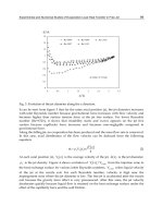
Fig. 1. Phase transition between the non-wave (dissipative) [left] and the wave
(non-dissipative) solution [right]. The critical transition point is at x
0
= Dk
0

= c/2. The
value of diffusity is taken D
= 1. The phase velocity w
f
of the wave-like propagation is
always smaller than the speed of light.
It can be recognized that there is a value of the wave number k when the discriminant changes
its sign in Equation (7) at the value k
0
= c/2D. Now, the solutions can be split into two
parts. On the one hand, we can consider the case k
> k
0
, when the solution is real and
wave-like (non-dissipative), and on the other hand, we take the case k
< k
0
, when the solution
is imaginary and non-wave (dissipative). The real and the imaginary part of the phase velocity
w
f
can be written for both cases
w
f
=
ω
k
= c

1 −

c
2
4D
2
k
2
< ck> k
0
, (9a)
158
Heat Conduction – Basic Research
Can a Lorentz Invariant Equation Describe Thermal Energy Propagation Problems? 5
Im w
f
=
ω
k
= c

c
2
4D
2
k
2
−1 k < k
0
.(9b)
The above physical discussion can be easily followed in Fig. 1.
In order to couple the thermal field given in Equation (2a) with other fields (like the inflaton

field in the cosmology shown in Sec. 4) it is worthy to reformulate it for this later use. It has
been shown in the literature (Márkus & Gambár, 2005) that the quantization of the thermal
field generates quasi particles and these particles may have a mass
M
0
=
¯h
2D
, (10)
where ¯h is the Planck constant. Moreover, the Planck units are applied for the present case
(c
= 1; ¯h = 1). Then the 3D Lagrangian given by Eq. (2a) should be rewritten
L
w
=
1
2
(Δϕ)
2
+
1
2

∂
2
ϕ
∂t
2

2

−
∂
2
ϕ
∂t
2
Δϕ −
1
2
M
4
0
ϕ
2
, (11)
where Δ is the Laplace operator.
3. Mechanical analogies for the two kinds of Klein-Gordon equations
It is instructive to study the set-up of the classical model of the Klein-Gordon equation
(Morse & Feshbach, 1953) to make comparisons and conclusions on the physical meaning
of the relevant terms that may appear similarly in a more general and abstract theory. The
mechanical model is a stretched string with little vertically oriented springs along the string
which pull back the spring to the equilibrium position as it is shown in Fig. 2(a). The equation
of motion of the string can be formulated applying the Lagrangian formalism. To achieve this,
the kinetic and potential energy terms are needed to calculate. The string has a kinetic energy
from its movement
T
=
1
2
A



∂Ψ
∂t

2
dx, (12)
where Ψ is the displacement from the equilibrium position,  is the density, A is the cross
section of the string. The mass element is dm
= Adx. The either of the potential energy
terms comes from the small deformation (elongation) of the stretching which is
V
= F

⎡
⎣

1 +

∂Ψ
∂x

2
−1
⎤
⎦
dx
∼
1
2

F


∂Ψ
∂x

2
dx, (13)
F is the stretching force. The other attractive potential energy term pertains to the little springs
which is
V
s
=
1
2
k
a

Ψ
2
dx. (14)
Here, k
a
is the spring direction coefficient density along the string as is shown in Fig 2(a). The
Lagrangian of the system can be formulated with the usual construction L
= T − V − V
s
,by
which the Euler-Lagrange equation as equation of motion — a Klein-Gordon equation with
positive "mass term" —

159
Can a Lorentz Invariant Equation Describe Thermal Energy Propagation Problems?
6 Will-be-set-by-IN-TECH
∂
2
Ψ
∂t
2
−
F
A
∂
2
Ψ
∂x
2
+
k
a
A
Ψ
= 0. (15)
can be deduced. Now, if a "repulsive" potential is imagined at the places of the springs shown
in Fig. 2(b) then a Klein-Gordon type equation with negative "mass term" (Gambár & Márkus,
2008) is obtained
∂
2
Ψ
∂t
2

−
F
A
∂
2
Ψ
∂x
2
−
k
a
A
Ψ
= 0. (16)
(a) A stretched string (green line) with
an additional attractive interaction by
the springs k
a
(b) A stretched string (green line) with
an additional "repulsive" interaction by
the springs k
a
(c) A stretched string (green line) on a
rotating disc; ω
0
is the angular velocity
Fig. 2. The three physical situations of the stretched string; the acting force is F for each cases.
The equations of motion due to the attractive or "repulsive" interactions pertain to the
different figures: Equation (15) for Fig. (a); Equation (16) for Fig. (b); Equation (18) for Fig.
(c).

The structure of this equation is exactly the same as in the case of Lorentz invariant thermal
energy propagation in Equation (5a). Since, it is clear from this mechanical example that the
negative sign of the third term in Equation (16) pertains to a repulsive interaction, thus, this is
the reson why the negative "mass term" may relate to a repulsive interaction in the relativistic
160
Heat Conduction – Basic Research
Can a Lorentz Invariant Equation Describe Thermal Energy Propagation Problems? 7
case in Equation (5a), in general. Maybe, it is complicated to prepare a device to ensure the
repulsive interaction from little springs. However, if the stretched string is placed on the
diameter of a rotating disk — shown in Fig. 2(c) that moves with the angular velocity ω
0
,then
the centrifugal force can produce the similar repulsive interaction.
The centrifugal potential of a point-like mass m moving on a circle with a radius r
−
1
2
mr
2
ω
2
0
can be generalized to the present case. This gives the potential V
rot
pertaining to the rotational
motion of the string
V
rot
= −
1

2
Aω
2
0

Ψ
2
dx. (17)
The relevant Lagrangian is L
= T −V −V
rot
, by which the calculated equation of motion can
be obtained
∂
2
Ψ
∂t
2
−
F
A
∂
2
Ψ
∂x
2
−ω
2
0
Ψ = 0. (18)

The same mathematical structure can be immediately recognized comparing this equation
with the Equations (5a) and (16). This means that these three equations must involve the
similar physical behavior: the spinodal instability and the dynamic phase transition (Gambár,
2010). All together these examples clearly prove the physical reality of the Klein-Gordon
equation with negative "mass term" in nature.
Finally, for the completeness the dispersion relation for Equation (18) can be also calculated
Ω
(k, ω
0
)=

F
A
k
2
−ω
2
0
. (19)
This formula shows again the same physical behavior clearly as it has been found in Equation
(6a). The phase velocity is
w
ph
=
Ω
k
=

F
A

−

ω
0
k

2
. (20)
It is easy to recognize that for small angular velocity ω
0
while

F
A
>
ω
0
k
(21)
is completed, then wave modes exist. The opposite case is when

F
A
<
ω
0
k
, (22)
there are no wave modes. The physical meaning is that, above a certain value of ω
0

,the
centrifugal force elongates the string to infinity, the string cannot have vibrating modes. The
change in the propagation modes is an angular velocity controlled dynamic phase transition
that divides the dissipative – non-dissipative transition like in Equations (7), (9a) and (9b) for
the thermal case.
161
Can a Lorentz Invariant Equation Describe Thermal Energy Propagation Problems?
8 Will-be-set-by-IN-TECH
4. Inflationary cosmology with the dynamic temperature
It is a great challenge to experience and understand how the Lorentz invariant propagating
thermal energy field ϕ can interact with other physical fields. In this way new physical
relations, considerations and explanations may be expected for the relevant phenomena.
As an advanced example, to point out the strength of the formulation, the thermal and
cosmological inflaton fields are coupled within the Lagrangian framework (Márkus et al.,
2009).
4.1 Linde’s model of the inflaton field
In the present model the cosmological model is based on the Einstein’s equation in the
Friedman-Robertson-Walker metric. Now, the action S can be expressed as
S
=


−
˜
gL
FRW
d
4
x, (23)
where the expression

√
−
˜
g
= a
3
is the Friedman-Robertson-Walker metric. Here, the a(t)=
R(t)/R
0
is taken as the ’radius’ of the universe. The Lagrange density function L
FRW
of the
inflaton field φ
L
FRW
=

1
2

∂φ
∂t

2
−
1
2a
2
(∇φ)
2

−V(φ)

(24)
is the starting point in the description;
∇is the gradient operator. Then, the equation of motion
for the inflaton can be calculated
∂
2
φ
∂t
2
−
1
a
2
Δφ + 3H
∂φ
∂t
= −
δV(φ)
δφ
, (25)
where δV
(φ)/δφ means a functional derivative. The Hubble parameter H(t) is defined by
H
=
˙
a
a
. (26)

The fate of the universe depends on the potential V
(φ). The hybrid inflation model suggested
by Linde (Felder et al., 1999; 2001; Linde, 1982; 1994) introduces an additional scalar field σ (in
fact the Higgs field) into the effective potential
V
(σ, φ)=−
1
2a
2
(
∇
φ
)
2
+
1
2
m
2
φ
2
+
1
2
g
2
φ
2
σ
2

+
1
4λ
(M
2
−λσ
2
)
2
. (27)
Here, the first term on the right hand side pertains to the second term — the space derivate
term — on the left hand side in Equation (25). The second term generates the inflation
process, the third one couples the inflaton field to the introduced additional field σ and the last
one produces mass generation through the spontaneous symmetry breaking. The canonical
momentum of the inflaton field can be calculated
Π
φ
=
∂L
FRW
∂
˙
φ
=
˙
φ. (28)
Then the Hamiltonian
˜
H of the field which is the energy density can be obtained
162

Heat Conduction – Basic Research
Can a Lorentz Invariant Equation Describe Thermal Energy Propagation Problems? 9
˜
H
= Π
φ
˙
φ
− L
FRW
=

1
2

∂φ
∂t

2
+
1
2a
2
(∇φ)
2
+ V(φ)

. (29)
It is often used different notations for
˜

H
˜
H
= 
φ
= T
00
, (30)
where T
00
is called as the time-time component of the energy-momentum tensor. Furthermore,
the Einstein’s equation can be expressed in the FRW metric as

˙
a
a

2
=
8πG
3
, (31)
where G is the gravitational constant and  is the mass density. Substituting the energy density

φ
and the Planck mass
M
pl
=


¯hc
8πG
(32)
into Equation (31) and applying Planck units, the Friedman’s equation can be written in the
following form
H
2
=
1
3M
2
pl

φ
, (33)
which corresponds to a flat universe. If it is assumed that the universe is growing
homogeneously in the space we can neglect those terms where the spatial derivates (
∇ and Δ)
appear in Equation (25), then an ordinary differential equation can be obtained
d
2
φ
0
dt
2
+ 3H
dφ
0
dt
= −

δV(φ
0
)
δφ
0
, (34)
the ’field variable’ φ
0
depends on the time parameter only. In this case the energy density 
φ
has a simplified form

φ
=

1
2

dφ
0
dt

2
+ V(φ)

, (35)
by which the equation H
2
=(1/3M
2

pl
)
φ
naturally also remains valid, i.e.,
H
2
=
1
3M
2
pl

1
2

dφ
0
dt

2
+ V(φ)

. (36)
Soon it will be seen that the above equations, (35) and (36), with the modifying effect of
the thermal field ϕ
0
will become those equations which are going to be considered as the
time-evolution equations of the inflaton field.
4.2 The coupling of the fields
The introduction of the dynamic temperature and the laws of thermodynamics into the theory

of cosmology requires the same mathematical frame of the description. Now, the tool is ready
163
Can a Lorentz Invariant Equation Describe Thermal Energy Propagation Problems?