Heat Conduction Basic Research Part 8 ppt

10 Will-be-set-by-IN-TECH
to make this willing. The interaction of the thermal potential field ϕ [see Equation (11)] and
the inflaton field φ [see Equation (24)] can be constructed by adding the Lagrangians of the
different fields
L
int
=

1
2a
4
(Δϕ)
2
+
1
2

∂
2
ϕ
∂t
2

2
−
1
a
2
∂
2
ϕ

∂t
2
Δϕ −
1
2
M
4
0
ϕ
2

+

1
2

∂φ
∂t

2
−
1
2a
2
(∇φ)
2
−V(φ, ϕ)

. (37)
This Lagrangian L

int
of the coupled inflaton-thermal field by the following interaction
potential can also realize the spontaneous symmetry breaking
V
(φ, ϕ)=
1
2
m
2
φ
2
+
1
2
g
2
0
φ
2
ϕ
2
, (38)
where m denotes the mass of the inflaton, and g
0
is the coupling constant, moreover, this
description can involve the temperature of the inflaton field (Márkus et al., 2009). This fact
is very interesting, since at this stage, there is no need for the Higgs field and the mass
generation.
After all, applying the calculus of variation, two Euler-Lagrange equations as equations of
motion are arisen from the variation with respect to the variables φ and ϕ

∂
2
φ
∂t
2
−
1
a
2
Δφ + 3
˙
a
a
∂φ
∂t
= −
δV(φ, ϕ)
δφ
, (39)
and
1
a
4
ΔΔ ϕ +
∂
4
ϕ
∂t
4
+ 6

˙
a
a
∂
3
ϕ
∂t
3
+
1
a
3
∂
2
(a
3
)
∂t
2
∂
2
ϕ
∂t
2
−
2
a
2
Δ
∂

2
ϕ
∂t
2
−
¨
a
a
3
Δϕ −2
˙
a
a
3
Δ
∂ϕ
∂t
− M
4
0
ϕ
=
δV(φ, ϕ)
δϕ
. (40)
An important remark is needed here. Since, for the cases when the Lagrangian
contains second order time derivatives the Hamiltonian
˜
H must be expressed as follows
(Gambár & Márkus, 1994; Márkus & Gambár, 1991),

˜
H
=
∂ϕ
∂t
∂L
∂
˙
ϕ
−
∂ϕ
∂t
∂
∂t
∂L
∂
¨
ϕ
+
∂
2
ϕ
∂t
2
∂L
∂
¨
ϕ
− L. (41)
By substituting the Lagrangian L

int
from Equation (37), the Hamiltonian — energy density
regarding the whole space with all interactions — can be calculated

φ,ϕ
=
˜
H
= −
∂ϕ
∂t
∂
3
ϕ
∂t
3
+
∂ϕ
∂t
∂
∂t

1
a
2

Δϕ
+
1
a

2
∂ϕ
∂t
∂
∂t
Δϕ
+
1
2

∂
2
ϕ
∂t
2

2
−
1
2a
4
(
Δϕ
)
2
+
1
2
M
4

0
ϕ
2
+
1
2

∂φ
∂t

2
+
1
2a
2
(
∇
φ
)
2
+ V(φ, ϕ). (42)
In the case of a rapidly growing universe in a homogeneous space, the terms containing the
operators
∇ and Δ can be omitted, thus the obtained field equations are simplified to the
following coupled nonlinear ordinary differential equations:
164
Heat Conduction – Basic Research
Can a Lorentz Invariant Equation Describe Thermal Energy Propagation Problems? 11
d
2

φ
0
dt
2
+ 3H
dφ
0
dt
= −

m
2
+ g
2
0
ϕ
2
0

φ
0
, (43)
d
4
ϕ
0
dt
4
+ 6H
d

3
ϕ
0
dt
3
= M
4
0
ϕ
0
+ g
2
0
φ
2
0
ϕ
0
(44)
and
H
2
=
1
3M
2
pl

1
2


d
2
ϕ
0
dt
2

2
−
dϕ
0
dt
d
3
ϕ
0
dt
3
+
1
2

dφ
0
dt

2
+
1

2
M
4
0
ϕ
2
0
+
1
2
m
2
φ
2
0
+
1
2
g
2
0
φ
2
0
ϕ
2
0

. (45)
Here, the field φ

0
and ϕ
0
depend on time only. The three coupled nonlinear ordinary
differential equations, Equations (43), (44) and (45), can be considered as the equations of
motion of the inflationary model. It is easy to recognize that Equation (45) can be considered
as the modified version of Friedman’s equation given in Equation (33). The temperature
generated by the thermal field ϕ
0
can then be expressed as [see Equation (4a) and taking
into account Equation (10) with Planck units]
T
=
d
2
ϕ
0
dt
2
+ M
2
0
ϕ
0
. (46)
4.3 On the time evolution of the fields
The mathematical and numerical examinations show that the solution of these coupled
differential equations describes fairly well the time evolution of the inflationary universe
including its thermodynamical behavior. Due to the complicated nonlinear Equations (43-45)
the solutions can be achieved by numerical calculations for the time-dependence of the scalar

fields and the dynamic temperature T. These equations are needed to solve simultaneously
for the scalar field φ
0
and the thermal potential ϕ
0
first. After then the time evolution equation
for the (thermo)dynamic temperature can be obtained.
In the present model there are two adjustable parameters, namely, the mass M
0
of the thermal
field and the coupling constant g
0
. The time scales of the temperature and the scalar inflaton
field can be synchronized by the change of values for these two parameters. The mass of
the scalar field m is chosen in the same order of magnitude as it is proposed by Linde Linde
(1994), namely, m
= 80GeV. The two fitted parameters are M
0
= 52.2GeV and g
0
= 0.12GeV.
It is important to set relevant initial conditions to find reasonable numerical solutions for
Equations (43) – (45). Thus, a big acceleration is assumed at the beginning of the expansion
and the thermal field has a given initial value. This results an initial value for the temperature
T
0
∼ 2.5 × 10
6
GeV ∼ 10
19

K. (Presently, the exact magnitude of the temperature has not too
much importance, since another value can be obtained by rescaling, i.e., it does not touch the
shape of the temperature function. However, it is sure, that this value is rather far from the
theoretically possible
∼ 1.4 ×10
32
K value (Lima & Trodden, 1996; Márkus & Gambár, 2004).)
In order to ensure the thermal and the inflaton field decay the first time derivatives of them
are needed to be negative.
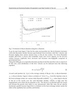
After finding a set of the numerical solutions, two main stages can be distinguished for the
time evolution of the inflaton field φ
0
. The first short period is when it decreases rapidly.
165
Can a Lorentz Invariant Equation Describe Thermal Energy Propagation Problems?
12 Will-be-set-by-IN-TECH
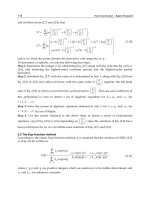
This follows the second rather long time interval in which the inflaton field oscillates with
decreasing amplitude. Both of these processes can be recognized well in Fig. 3.
0.02 0.04 0.06 0.08 0.10
t
50
100
150
Φ
0
t
Fig. 3. The time evolution of the inflaton field φ
0
(t) is shown. The short decreasing
(deacying) period is followed by a rather long damped oscillating process. Time is in

arbitrary units.
0.01 0.02 0.03 0.04 0.05 0.06 0.07 0.08
t
200
400
600
800

0
t
Fig. 4. The time evolution of the thermal field ϕ
0
(t). The field decays in the first period and
reaches its minimal value. It begins to increase monotonically when the inflaton field φ
0
(t)
starts to oscillate. Time is in arbitrary units.
It is noticable that the above described behavior of the inflaton field is in line with Linde’s
cosmology model (Felder et al., 2002; Linde, 1982; 1990; 1994) based on a potential energy
expression given by V
(φ
0
)=(m
2
/2)φ
2
0
+ V
0
with V

0
> 0 which is similar to Equation
(38), here. The physically coupled thermal field ϕ
0
produces a completely different behavior.
During inflation era, the field ϕ
0
decreases. Probably, the reason of this effect is strongly the
radius and the volume increase of the universe. Once it reaches a minimum which happens
about the same time when field φ
0
starts to oscillate. After then, the thermal field increases
166
Heat Conduction – Basic Research
Can a Lorentz Invariant Equation Describe Thermal Energy Propagation Problems? 13
monotonically since the decaying inflaton field φ
0
with a time delay pumps up it as plotted in
Fig. 4.
The temperature field T is coupled to the thermal field ϕ
0
by Equation (46), thus
mathematically this can be obtained directly. The time evolution of the temperature can be
followed in Fig. 5. In the first era of the inflation process the temperature decreases. After
reaching its minimal value, which is at the same instantaneous of the minimum of the thermal
field, it increases quite rapidly. This period of the cosmology is known as the reheating process
of the universe. The present elaboration of the model can describe and reproduce to this stage
of the life of the early universe.
0.01 0.02 0.03 0.04 0.05 0.06 0.07 0.08
t

500 000
1.0 10
6
1.5 10
6
2.0 10
6
2.5 10
6
T t
Fig. 5. The time evolution of the temperature field T(t). The temperature follows the change
of the thermal field ϕ
0
. It decreases in the first period of the expansion while its reaches a
minimal value. The, due to the pumping of the inflaton field φ
0
into the thermal field ϕ
0
,the
temperature starts increasing. This growing temperature period can be identified as the
reheating process in Linde’s cosmology model. Time is in arbitrary units.
0.01 0.02 0.03 0.04 0.05
t
2 10
12
4 10
12
6 10
12
8 10

12
1 10
13
Ρ
Φ
0
,
0
t
Fig. 6. The time evolution of the energy density ρ
φ
0
ϕ
0
(t). As it is expected the energy density
decreases monotonically during the expansion. Time is in arbitrary units.
Since the whole energy of the universe is conserved during the expansion, the energy density
is needed to decrease. This tendency can be seen in Fig. 6. Finally, the radius a
(t) of the
universe is plotted in Fig. 7.
167
Can a Lorentz Invariant Equation Describe Thermal Energy Propagation Problems?
14 Will-be-set-by-IN-TECH
0.01 0.02 0.03 0.04 0.05
t
0.02
0.04
0.06
0.08
0.10

at
Fig. 7. The time evolution of the radius a(t) of the universe. As it is expected the radius
increases monotonically during the expansion. Time is in arbitrary units.
The presented model of the inflationary period is not complete in that sense that e.g., the
Higgs mechanism is dropped by the elimination of the fourth term of the effective potential in
Equation (27) comparing with the applied potential in Equation (38). However, hopefully, the
strength of the theory can be read out from the most spectacular results: the thermal field can
generate not only the spontaneous symmetry breaking involving the correct time evolution
of the inflaton field, but it ensures a really dynamic Lorentz invariant thermodynamic
temperature. The further development of this cosmological model would be to add the
particle generator Higgs mechanism again.
5. Wheeler propagator of the Lorentz invariant thermal energy propagation
As it has been shown previously that the Lorentz invariant description involves different
physically realistic propagation modes. However, the development of the theory is needed
to learn more about propagation, the transition amplitude and the completeness of causality,
i.e., the field equation in Equation (5a) does not violate the causality principle.
5.1 The Green function
A common way to examine these questions is based on the Green function method.
Mathematically, the solution of the equation
1
c
2
∂
2
G
∂t
2
−
∂
2

G
∂x
2
−
c
2
c
2
v
4λ
2
G = −δ
n
(x − x

) (47)
for the Green function G is needed to find. The n-dimensional source function is δ
n
(x − x

)=
δ
n−1
(r − r

)δ(t −t

) which can be expressed by the delta function
δ
n

(x − x

)=
1
(2π)
n

d
n
ke
ik(x−x

)
. (48)
Here, the vector k
=(k, ω
0
) is n-dimensional; the n − 1dimensionalk pertains to the space
and the 1-dimensional ω
0
is to time. Moreover, the d’Alembert operator is
168
Heat Conduction – Basic Research
Can a Lorentz Invariant Equation Describe Thermal Energy Propagation Problems? 15

=
1
c
2
∂

2
∂t
2
−Δ. (49)
To shorten the formulations the following abbreviation is also introduced
m
2
=
c
2
c
2
v
4λ
2
. (50)
Now, Equation (47) has a simpler form
(

−m
2
)G = δ
n
(x − x

). (51)
Since, the equality holds
(

−m

2
)
−1
e
ik(x−x

)
= −
e
ik(x−x

)
k
2
−m
2
, (52)
then we obtain
(

−m
2
)
−1
δ
n
(x − x

)=−
1

(2π)
n

d
n
k
e
ik(x−x

)
k
2
−m
2
. (53)
After all, the Green function can be formally expressed as
G
(x, x

)=
1
(2π)
n

d
n
k
e
ik(x−x


)
k
2
−m
2
. (54)
To calculate this integral the zerus points of the denominator k
2
−m
2
= p
2
− p
2
0
−m
2
= 0are
needed, from which
p
0
= ±

p
2
−m
2
. (55)
can be obtained. After then, the propagator should be expressed in proper way taking
Equation (54)

G
(p)=
1
p
2
− p
2
0
−m
2
. (56)
In the sense of the theory the retarded G
ret
(p)=1/(p
2
− p
2
0
−m
2
)
ret
and the advanced
G
adv
(p)=1/(p
2
− p
2
0

−m
2
)
adv
propagators are needed to be expressed for the tachyons due
to the presence of the imaginary poles. Now, the construction of the Wheeler propagator
(Wheeler, 1945; 1949) can be expounded as a half sum of the above propagators
G
(p)=
1
2
G
adv
(p)+
1
2
G
ret
(p). (57)
5.2 The Bochner’s theorem
The calculation of propagators is based on the Bochner’s theorem (Bochner, 1959;
Bollini & Giambiagi, 1996; Bollini & Rocca, 1998; 2004; Jerri, 1998). It states that if the function
f
(x
1
, x
2
, , x
n
) depends on the variable set (x

1
, x
2
, ,x
n
) then its Fourier transformed is —
without the factor 1/
(2π)
n/2
—
169
Can a Lorentz Invariant Equation Describe Thermal Energy Propagation Problems?
16 Will-be-set-by-IN-TECH
g(y
1
, y
2
, ,y
n
)=

d
n
xf(x
1
, x
2
, , x
n
)e

ix
i
y
i
(i = 1, ,n). (58)
However, it is useful to introduce the variables x
=(x
2
1
+ x
2
2
+ + x
2
n
)
1/2
and y =(y
2
1
+
y
2
2
+ + y
2
n
)
1/2
instead of the original sets. Now, the examinations are restricted to the

spherically symmetric functions f
(x) and g(y ). In these cases the above Fourier transform
given by Equation (58) can be calculated by applying the Hankel (Bessel) transformation by
which we obtain
g
(y, n)=
(
2π)
n/2
y
n/2−1

∞
0
f (x)x
n/2
J
n/2−1
(xy)dx. (59)
Here, J
α
is a first kind α order Bessel function. Later it will be very useful to calculate the
function f with causal functions depending on the momentum space p thus we write
f
(x, n)=
(
2π)
n/2
x
n/2−1


∞
0
g(p)p
n/2
J
n/2−1
(xp)dp. (60)
It can be seen that the singularity at the origin depends on n analytically.
5.3 Calculation of the Wheeler propagator
To obtain the Wheeler propagator, first, e.g., the integral in Equation (54) for the advanced
propagator can be calculated
G
adv
(x)=
1
(2π)
n

d
n−1
pe
ipr

adv
dp
0
e
−ip
0

x
0
p
2
− p
2
0
−m
2
. (61)
The path of integration runs parallel to the real axis and below both the poles for the advanced
propagator. (For the retarded propagator the path runs above the poles.) Thus, considering
the propagator G
adv
(p) for x
0
> 0 the path is closed on the lower half plane giving null result.
In the opposite case, when x
0
< 0, there is a non-zero finite contribution of the residues at the
poles
p
0
= ±ω =

p
2
−m
2
if p

2
≥ m
2
(62)
and
p
0
= ±iω

=

p
2
−m
2
if p
2
≤ m
2
. (63)
After applying the Cauchy’s residue theorem for the integration with respect to p
0
we obtain
an n
−1 order integral
G
adv
(x)=−
H(−x
0

)
(2π)
n−1

d
n−1
pe
ipr
si n [(p
2
−m
2
+ i0)
1
2
x
0
]
(p
2
−m
2
+ i0)
1
2
, (64)
where H is the Heaviside’s function. The retarded propagator can be similarly obtained
G
ret
(x)=

H(x
0
)
(2π)
n−1

d
n−1
pe
ipr
si n [(p
2
−m
2
+ i0)
1
2
x
0
]
(p
2
−m
2
+ i0)
1
2
. (65)
170
Heat Conduction – Basic Research

Can a Lorentz Invariant Equation Describe Thermal Energy Propagation Problems? 17
Considering the form of the propagator in Equation (57) and taking the propagators in
Equations (64) and (65) we obtain the Wheeler-propagator
G
(x)=
Sgn(x
0
)
2(2π)
n−1

d
n−1
pe
ipr
si n [(p
2
−m
2
+ i0)
1
2
x
0
]
(p
2
−m
2
+ i0)

1
2
. (66)
To evaluate the above propagators the integrals can be rewritten by the Hankel transformation
based on Bochner’s theorem [Equation (59)]
1
(2π)
n−1

d
n−1
pe
ipr
si n [(p
2
−m
2
+ i0)
1
2
x
0
]
(p
2
−m
2
+ i0)
1
2

=
1
(2π)
n−1
2
1
x
n−1
2
−1

∞
0
p
n−1
2
sin(p
2
−m
2
)
1
2
x
0
(p
2
−m
2
)

1
2
J
n−1
2
−1
(xp) dp, (67)
where p
=

p
2
1
+ p
2
2
+ + p
2
n
−1
and r =

x
2
1
+ x
2
2
+ + x
2

n
−1
. The following integrals
(Gradshteyn & Ryzhik, 1994) are applied for the above calculations such as

∞
0
dy y
γ+1
sin

a

b
2
+ y
2


b
2
+ y
2
J
γ
(cy)=

π
2
b

1
2
+γ
c
γ
(a
2
−c
2
)
−
1
4
−
1
2
γ
J
−γ−
1
2
(b

a
2
−c
2
), (68)
if 0
< c < a, Re b > 0, −1 < Re γ < 1/2, and


∞
0
dy y
γ+1
sin

a

b
2
+ y
2


b
2
+ y
2
J
γ
(cy)=0, (69)
if 0
< a < c, Re b > 0, −1 < Re γ <
1
2
. The parameters of the model can be fitted by
a
= x
0

, b = im = i
cc
v
2λ
, c
= r, γ =
n
2
−
3
2
. (70)
and we consider the relation between the Bessel functions
J
α
(ix)=i
α
I
α
(x), (71)
where I
α
(x) is the modified Bessel function. Now, we can express the advanced Wheeler
propagator Equation (64) of the tachyonic thermal energy propagation
W
adv
(x)=H(−x
0
)
π

(2π)
n/2

cc
v
2λ

n
2
−1
(x
2
0
−r
2
)
1
2
(1−
n
2
)
+
I
1−
n
2

cc
v

2λ
(x
2
0
−r
2
)
1
2
+

. (72)
The calculation for the retarded propagator can be similarly elaborated by Equations (65) and
(67)
W
ret
(x)=H(x
0
)
π
(2π)
n/2

cc
v
2λ

n
2
−1

(x
2
0
−r
2
)
1
2
(1−
n
2
)
+
I
1−
n
2

cc
v
2λ
(x
2
0
−r
2
)
1
2
+


. (73)
Comparing the results of Equations (72) and (73) it can be seen that we can write one common
formula easily to express the complete propagator. Thus the Wheeler-propagator in the n
dimensional space-time — remembering the construction in Equation (57) — is
171
Can a Lorentz Invariant Equation Describe Thermal Energy Propagation Problems?
18 Will-be-set-by-IN-TECH
W
(n)
(x)=
π
2(2π)
n/2

cc
v
2λ

n
2
−1
(x
2
0
−r
2
)
1
2

(1−
n
2
)
+
I
1−
n
2

cc
v
2λ
(x
2
0
−r
2
)
1
2
+

. (74)
The calculated Wheeler propagator in the 3
+ 1 dimensional space-time can be expressed for
the thermal energy propagation
W
(4)
(r, x

0
)=
1
8π

cc
v
2λ

(x
2
0
−r
2
)
−
1
2
I
−1

cc
v
2λ
(x
2
0
−r
2
)

1
2

. (75)
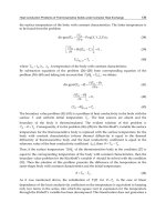
The expected causality can be immediately recognized from the plot of the propagator in Fig.
8, since it differs to zero just within the light cone.
10
5
0
5
10
r
10
5
0
5
10
t
0
10
20
30
W r, t
Fig. 8. The causal Wheeler propagator in the space-time — in arbitrary units — which is zero
out of the light cone.
Finally, it is important to mention and emphasize that the participating particles of the above
treated thermal energy propagation cannot be observable directly as Bollini’s and Rocca’s
detailed studies (Bollini & Rocca, 1997a;b; Bollini et al., 1999) show. This is a consequence
of the fact that the tachyons do not move as free particles, thus they can be considered as
the mediators of the dynamic phase transition (Gambár & Márkus, 2007; Márkus & Gambár,

2010).
6. Summary and concluding remarks
This chapter of the book is dealing with the hundred years old open question of how it
could be formulated and exploited the Lorentz invariant description of the thermal energy
propagation. The relevant field equation as the leading equation of the theory providing the
finite speed of action is a Klein-Gordon type equation with negative "mass term". It has been
shown via the dispersion relations that the classical Fourier heat conduction equation is also
involved, naturally. The tachyon solution of this kind of Klein-Gordon equation ensures that
both wave-like (non-dissipative, oscillating) and the non-wave-like (dissipative, diffusive)
signal propagations are present. The two propagation modes are divided by a spinodal
instability pertaining to a dynamic phase transition. It is important to emphasize that in this
172
Heat Conduction – Basic Research
Can a Lorentz Invariant Equation Describe Thermal Energy Propagation Problems? 19
way, finally, the concept of the dynamic temperature has been introduced.
Then, a mechanical system is discussed to point out clearly that Klein-Gordon equations with
the same mathematical structure and similar physical meaning can be found in the other
disciplines of physics, too. The model involves a stretched string put on the diameter of a
rotating disc. Collecting the kinetic and potential energy terms and formulating the Lagrange
function of the problem, it has been shown that the equation of motion as Euler-Lagrange
equation is exactly the above mentioned Klein-Gordon equation. The calculated dispersion
relation points out unambiguously that the dynamics is similar to the case of Lorentz invariant
heat conduction. The motion is vibrating (oscillating) below a system parameter dependent
angular velocity, or diffusive (decaying) above this value.
The great challenge is to embed the concept of dynamic temperature into the general
framework of physics. One of the aims via this step is to introduce the second law of
thermodynamics by which the most basic law of nature may appear in the physical theories.
Thus, such categories like dissipation, irreversibility, direction of processes can be handled
directly within a description. This was the motivation to elaborate the coupling of the inflaton
and the thermal field. As it can be concluded from the results, the introduced thermal field can

generate the spontaneous symmetry breaking in the theory — without the Higgs mechanism
— due to its property including the spinodal instability and the dynamic phase transition.
The inflation decays into the thermal field by which the reheating process can start during
the expansion of the universe. The time evolution of the inflation field is reproduced so well
as it is known from the relevant cosmological models. It is important to emphasize that the
thermal field generates a really dynamic temperature. A further progress could be achieved
by the adding again the Higgs mechanism to generate massive particles in the space. This
elaboration of the model remains for a future work.
Finally, it is an important step to justify that the above theory of thermal propagation
completes the requirement of the causality. This question comes up due to the tachyon
solutions. The arisen doubts can be eliminated in the knowledge of the propagator of the
process. The relevant causal Wheeler propagator can be deduced by a longer, direct, analytic
mathematical calculation applying the Bochner’s theorem. The results clearly shows that
the causality is completed since the propagator is within the light cone, i.e., the theory is
consistent.
The presented theory of this chapter is put into the general framework of the physics
coherently. These results mean a good base how to couple the thermodynamic field with the
other fields of physics. Hopefully, it opens new perspectives towards in the understanding of
irreversibility and dissipation in the field theoretical processes.
7. Acknowledgment
This work is connected to the scientific program of the " Development of quality-oriented and
harmonized R+D+I strategy and functional model at BME" project. This project is supported
by the New Hungary Development Plan (Project ID: TÁMOP-4.2.1/B-09/1/KMR-2010-0002).
8. References
Anderson C. D. R. & Tamma, K. K. (2006). Novel heat conduction model for bridging different
space and time scales. Physical Review Letters, Vol. 96, No. 18, (May 2006) p. 184301,
ISSN 0031-9007
173
Can a Lorentz Invariant Equation Describe Thermal Energy Propagation Problems?
20 Will-be-set-by-IN-TECH

Bochner, S. (1959). Lectures on Fourier Integrals, Princeton Univ., ISBN 0691079943, New Jersey,
USA.
Bollini, C. G. & Giambiagi, J. J. (1996). Dimensional regularization in configuration space.
Physical Review D, Vol. 53, No. 10, (May 1996) pp. 5761-5764, ISSN 0556-2821
Bollini, C. G. & Rocca, M. C. (1997). Vacuum state of the quantum string without anomalies in
any number of dimensions. Nuovo Cimento A, Vol. 110, No. 4, (April 1997) pp. 353-361,
ISSN 0369-3546
Bollini, C. G. & Rocca, M. C. (1997). Is the Higgs a visible particle? Nuovo Cimento A, Vol. 110,
No. 4, (April 1997) pp. 363-367, ISSN 0369-3546
Bollini, C. G. & Rocca, M. C. (1998). Wheeler propagator. International Journal of Theoretical
Physics, Vol. 37, No. 11, (November 1998) pp. 2877-2893, ISSN 0020-7748
Bollini, C. G., Oxman L. E. & M. C. Rocca, M. C. (1999). Coupling of tachyons to
electromagnetism International Journal of Theoretical Physics,Vol.38,No.2,(February
1999) pp. 777-791, ISSN 0020-7748
Bollini, C. G. & Rocca, M. C. (2004). Convolution of Lorentz invariant ultradistributions and
field theory. International Journal of Theoretical Physics, Vol. 43, No. 4, (April 2004) pp.
1019-1051, ISSN 0020-7748
Borsányi, Sz., Patkós, A., Polónyi, J. & Szép, Zs. (2000). Fate of the classical false vacuum.
Physical Review D, Vol. 62, No. 8, (October 2000) p. 085013, ISSN 0556-2821
Borsányi, Sz., Patkós, A & Sexty, D. (2002). Goldstone excitations from spinodal instability.
Physical Review D, Vol. 66, No. 2, (July 2002) p. 025014, ISSN 0556-2821
Borsányi, Sz., Patkós, A & Sexty, D. (2003). Nonequilibrium Goldstone phenomenon in
tachyonic preheating. Physical Review D, Vol. 68, No. 6, (September 2003) p. 063512,
ISSN 0556-2821
Cahill, D. G., Ford, W. K., Goodson, K. E., Mahan, G. D., Mahumdar, A., Maris, H. J., Merlin,
R. & Phillpot, S. R. (2003). Nanoscale thermal transport. Journal of Applied Physics,Vol.
93, No. 2, (January 2003) pp. 793-818, ISSN 0021-8979
Chen, G. (2001). Ballistic-diffusive heat-conduction equations. Physical Review Letters,Vol.86,
No. 11, (March 2001) pp. 2297-2300, ISSN 0031-9007
Eckart, C. (1940). The thermodynamics of irreversible processes. III. Relativistic theory of the

simple fluid. Physical Review, Vol. 58, No. 10, (November 1940) pp. 919-924
Felder, G., Kofman, L. & Linde, A. D. (1999). Inflation and preheating in nonoscillatory
models. Physical Review D, Vol. 60, No. 10, (November 1999) p. 103505, ISSN
0556-2821
Felder, G., Kofman, L. & Linde, A. D. (2001). Tachyonic instability and dynamics of
spontaneous symmetry breaking Physical Review D, Vol. 64, No. 12, (December 2001)
p. 103505, ISSN 0556-2821
Felder, G., Frolov, A., L. Kofman, L. & Linde, A. (2002). Cosmology with negative potentials.
Physical Review D, Vol. 66, No. 2, (July 2002) p. 023507, ISSN 0556-2821
Gambár, K. & Márkus, F. (1994). Hamilton-Lagrange formalism of nonequilibrium
thermodynamics. Physical Review E, Vol. 50, No. 2, (August 1994) pp. 1227-1231, ISSN
1063-651X
Gambár, K. (2005). Least action principle for dissipative processes, pp. 245-266, in Variational and
Extremum Principles in Macroscopic Systems (Eds. Sieniutycz, S. & Farkas, H.), Elsevier,
ISBN 0080444881, Oxford.
174
Heat Conduction – Basic Research
Can a Lorentz Invariant Equation Describe Thermal Energy Propagation Problems? 21
Gambár, K. & Márkus, F. (2007). A possible dynamical phase transition between the
dissipative and the non-dissipative solutions of a thermal process. Physics Letters A,
Vol. 361, No. 4-5, (February 2007) pp. 283-286, ISSN 0375-9601
Gambár, K. & Márkus, F. (2008). A simple mechanical model to demonstrate a dynamical
phase transition. Reports on Mathematical Physics, Vol. 62, No. 2, (October 2008) pp.
219-227, ISSN 0034-4877
Gambár, K. (2010). Change of the dynamics of the systems: dissipative – non-dissipative
transition. Informatika, Vol. 12, No. 2, (2010) pp. 23-26, ISSN 1419-2527
Gradshteyn, S. & Ryzhik, I. M. (1994). Tables of Integrals, Series, and Products, Academic Press,
ISBN 012294755X, San Diego.
Jerri, A. J. The Gibbs Phenomenon in Fourier Analysis, splines, and wavelet approximations,Kluwer,
ISBN 0792351096, Dordrecht.

Joseph, D. D. & Preziosi, L. (1989). Heat waves. Reviews of Modern Physics, Vol. 61, No. 1,
(January 1989) pp. 41-73, ISSN 0034-6861
Jou, D., Casas-Vázquez & Lebon, G. (2010). Extended irreversible thermodynamics,Springer,
ISBN 9789048130733, New York, USA.
Lima, J. A. S. & Trodden , M. (1996). Decaying vacuum energy and deflationary cosmology
in open and closed universes. Physical Review D, Vol. 53, No. 8, (April 1996) pp.
4280-4286, ISSN 0556-2821
Linde, A. D. (1982). A new inflationary universe scenario — A possible solution of the horizon,
flatness, homogeneity, isotropy and primordial monopole problems. Physics Letters B,
Vol. 108, No. 6, (February 1982) pp. 389-393, ISSN 0370-2693
Linde, A. D. (1990). Particle Physics and Inflationary Cosmology , Harwood Academic Publishers,
ISBN 3718604892, Chur, Switzerland.
Linde, A. D. (1994). Hybrid inflation. Physical Review D, Vol. 49, No. 2, (January 1994) pp.
748-754, ISSN 0556-2821
Liu, W. & Asheghi, M. (2004). Phonon-boundary scattering in ultrathin single-crystal silicon
layers. Applied Physics Letters, Vol. 84, No. 19, (May 2004) pp. 3819-3821, ISSN
0003-6951
Ma, S k. (1982). Modern Theory of Critical Phenomena, Addison-Wesley, ISBN 0805366717,
California, USA.
Márkus, F. & Gambár, K. (1991). A variational principle in the thermodynamics. Journal
of Non-Equilibrium Thermodynamics, Vol. 16, No. 1, (March 1991) pp. 27-31, ISSN
0340-0204
Márkus, F. & Gambár, K. (2004). Derivation of the upper limit of temperature from the field
theory of thermodynamics. Physical Review E, Vol. 70, No. 5, (November 2004) p.
055102(R), ISSN 1063-651X
Márkus, F. (2005). Hamiltonian formulation as a basis of quantized thermal processes, pp. 267-291,
in Variational and Extremum Principles in Macroscopic Systems (Eds. Sieniutycz, S. &
Farkas, H.), Elsevier, ISBN 0080444881, Oxford, England.
Márkus, F. & Gambár, K. (2005). Quasiparticles in a thermal process. Physical Review E,Vol.71,
No. 2, (June 2005) p. 066117, ISSN 1539-3755

Márkus, F., Vázquez, F. & Gambár, K. (2009). Time evolution of thermodynamic temperature
in the early stage of universe. Physica A, Vol. 388, No. 11, (June 2009) pp. 2122-2130,
ISSN 0378-4371
175
Can a Lorentz Invariant Equation Describe Thermal Energy Propagation Problems?
22 Will-be-set-by-IN-TECH
Márkus, F. & Gambár, K. (2010). Wheeler propagator of the Lorentz invariant thermal energy
propagation. International Journal of Theoretical Physics,Vol.49,No.9,(September
2010) pp. 2065-2073, ISSN 0020-7748
Morse, Ph. M. & Feshbach, H. (1953). Methods of Theoretical Physics, McGraw-Hill, New York,
USA.
Sandoval-Villalbazo, A. & García-Colín L. S. (2000). The relativistic kinetic formalism
revisited. Physica A Vol. 278, No. 3-4, (April 2000) pp. 428-439, ISSN 0378-4371
Schwab, K., Henriksen, E. A., Worlock, J. M. & Roukes, M. L. (2000). Measurement of the
quantum of thermal conductance. Nature, Vol. 404, No. 6781, (April 2000) pp. 974-977,
ISSN 0028-0836
Sieniutycz, S. (1994). Conservation laws in variational thermo-hydrodynamics,KluwerAcademic
Publishers, ISBN 0792328027, Dordrecht, The Netherlands.
Sieniutycz, S. & Berry, R. S. (2002). Variational theory for thermodynamics of thermal waves.
Physical Review E, Vol. 65, No. 4, (April 2002) p. 046132, ISSN 1063-651X
Vázquez, F., Márkus, F. & Gambár, K. (2009). Quantized heat transport in small systems: A
phenomenological approach. Physical Review E, Vol. 79, No. 3, (March 2009) p. 031113,
ISSN 1539-3755
Wheeler, J. A. & Feynman, R. P. (1945). Interaction with the absorber as the mechanism of
radiation Reviews of Modern Physics, Vol. 17, No. 2-3, (April-July 1945) pp. 157-181
Wheeler, J. A. & Feynman, R. P. (1949). Classical electrodynamics in terms of direct
interparticle action. Reviews of Modern Physics, Vol. 21, No. 3, (July 1949) pp. 425-433
176
Heat Conduction – Basic Research
8

Time Varying Heat Conduction in Solids
Ernesto Marín Moares
Centro de Investigación en Ciencia Aplicada y Tecnología Avanzada (CICATA)
Unidad Legaria, Instituto Politécnico Nacional (IPN)
México
1. Introduction
People experiences heat propagation since ancient times. The mathematical foundations of
this phenomenon were established nearly two centuries ago with the early works of Fourier
[Fourier, 1952]. During this time the equations describing the conduction of heat in solids
have proved to be powerful tools for analyzing not only the transfer of heat, but also an
enormous array of diffusion-like problems appearing in physical, chemical, biological, earth
and even economic and social sciences [Ahmed & Hassan, 2000]. This is because the
conceptual mathematical structure of the non-stationary heat conduction equation, also
known as the heat diffusion equation, has inspired the mathematical formulation of several
other physical processes in terms of diffusion, such as electricity flow, mass diffusion, fluid
flow, photons diffusion, etc [Mandelis, 2000; Marín, 2009a]. A review on the history of the
Fourier´s heat conduction equations and how Fourier´s work influenced and inspired others
can be found elsewhere [Narasimhan, 1999].
But although Fourier´s heat conduction equations have served people well over the last two
centuries there are still several phenomena appearing often in daily life and scientific
research that require special attention and carefully interpretation. For example, when very
fast phenomena and small structure dimensions are involved, the classical law of Fourier
becomes inaccurate and more sophisticated models are then needed to describe the thermal
conduction mechanism in a physically acceptable way [Joseph & Preziosi, 1989, 1990].
Moreover, the temperature, the basic parameter of Thermodynamics, may not be defined at
very short length scales but only over a length larger than the phonons mean free paths,
since its concept is related to the average energy of a system of particles [Cahill, et al., 2003;
Wautelet & Duvivier, 2007]. Thus, as the mean free path is in the nanometer range for many
materials at room temperature, systems with characteristic dimensions below about 10 nm
are in a nonthermodynamical regime, although the concepts of thermodynamics are often

used for the description of heat transport in them. To the author´s knowledge there is no yet
a comprehensible and well established way to solve this very important problem about the
definition of temperature in such systems and the measurement of their thermal properties
remains a challenging task. On the other hand there are some aspects of the heat conduction
through solids heated by time varying sources that contradict common intuition of many
people, being the subject of possible misinterpretations. The same occurs with the
understanding of the role of thermal parameters governing these phenomena.

Heat Conduction – Basic Research
178
Thus, this chapter will be devoted to discuss some questions related to the above mentioned
problems starting with the presentation of the equations governing heat transfer for
different cases of interest and discussing their solutions, with emphasis in the role of the
thermal parameters involved and in applications in the field of materials thermal
characterization.
The chapter will be distributed as follows. In the next section a brief discussion of the
principal mechanisms of heat transfer will be given, namely those of convection, radiation
and conduction. Emphasis will be made in the definition of the heat transfer coefficients for
each mechanism and in the concept of the overall heat transfer coefficient that will be used
in later sections. Section 2 will be devoted to present the general equation governing non-
stationary heat propagation, namely the well known (parabolic) Fourier’s heat diffusion
equation, in which further discussions will be mainly based. The conditions will be
discussed under which this equation can be applied. The modified Fourier’s law, also
known as Cattaneo’s Equation [Cattaneo, 1948], will be presented as a useful alternative
when the experimental conditions are such that it becomes necessary to consider a
relaxation time or build-up time for the onset of the thermal flux after a temperature
gradient is suddenly imposed on the sample. Cattaneo’s equation leads them to the
hyperbolic heat diffusion equation. Due to its intrinsic importance it will be discussed with
some detail. In Section 3 three important situations involving time varying heat sources will
be analyzed, namely: (i) a sample periodically and uniformly heated at one of its surfaces,

(ii) a finite sample exposed to a finite duration heat pulse, and (iii) a finite slab with
superficial continuous uniform thermal excitation. In each case characteristic time and
length scales will be defined and discussed. Some apparently paradoxical behaviors of the
thermal signals and the role playing by the characteristic thermal properties will be
explained and physical implications in practical fields of applications will be presented too.
In Section 4 our conclusions will be drawn.
2. Heat transfer mechanisms
Any temperature difference within a physical system causes a transfer of heat from the
region of higher temperature to the one of lower. This transport process takes place until the
system has become uniform temperature throughout. Thus, the flux of heat,

(units of W),
should be some function of the temperatures, T
l
and T
2
, of both the regions involved (we
will suppose that T
2
> T
1
). The mathematical form of the heat flux depends on the nature of
the transport mechanism, which can be convection, conduction or radiation, or a coupling of
them. The dependence of the heat flux on the temperature is in general non linear, a fact that
makes some calculations quite difficult. But when small temperature variations are
involved, things become much simpler. Fortunately, this is the case in several practical
situations, for example when the sun rays heat our bodies, in optical experiments with low
intensity laser beams and in the experiments that we will describe here later.
Heat convection takes place by means of macroscopic fluid motion. It can be caused by an
external source (forced convection) or by temperature dependent density variations in the

fluid (free or natural convection). In general, the mathematical analysis of convective heat
transfer can be difficult so that often the problems can be solved only numerically or
graphically [Marín, et al., 2009]. But convective heat flow, in its most simple form, i.e. heat
transfer from surface of wetted area A and temperature T
2
, to a fluid with a temperature T
1
,

Time Varying Heat Conduction in Solids
179
for small temperature differences, T=T
2
-T
1
, is given by the (linear with temperature)
Newton’s law of cooling,

conv
=h
conv
T (1)
The convective heat transfer coefficient, h
conv
, is a variable function of several parameters of
different kinds but independent on T.
On the other hand heat radiation is the continuous energy interchange by means of
electromagnetic waves. For this mechanism the net rate of heat flow,

rad

, radiated by a
body surrounded by a medium at a temperature T
1
, is given by the Stefan-Boltzmann Law.

rad
= e A(T
2
4
- T
1
4
) (2)
where

is the Stefan-Boltzmann constant, A is the surface area of the radiating object and e
is the total emissivity of its surface having absolute temperature T
2
.
A glance at Eq. (2) shows that if the temperature difference is small, then one should expand
it as Taylor series around T
1
obtaining a linear relationship:


rad
=4

e A T
1

3
(T
2
-T
1
)=h
rad
T (3)
If we compare this equation with Eq. (1) we can conclude that in this case h
rad
=4

e A T
1
3
can
be defined as a radiation heat transfer coefficient.
On the other hand, heat can be transmitted through solids mainly by electrical carriers
(electrons and holes) and elementary excitations such as spin waves and phonons (lattice
waves). The stationary heat conduction through the opposite surfaces of a sample is
governed by Fourier’s Law


cond
=-kAT (4)
The thermal conductivity, k (W/mK), is expressed as the quantity of heat transmitted per
unit time, t, per unit area, A, and per unit temperature gradient. For one-dimensional steady
state conduction in extended samples of homogeneous and isotropic materials and for small
temperature gradients, Fourier’s law can be integrated in each direction to its potential form.
In rectangular coordinates it reads:

Φ

=








=
∆

=
∆


=ℎ

∆ (5)
Here T
l
and T
2
represent two planar isotherms at positions x
1
and x
2
, respectively, L=x

2
-x
1
,
and


=


=



(6)
is the thermal resistance against heat conduction (thermal resistance for short) of the sample.
The Eq. (5) is often denoted as Ohm’s law for thermal conduction following analogies
existing between thermal and electrical phenomena. Comparing with Eq. (1) we see that the
parameter h
cond
has been incorporated in Eq. (6) as the conduction heat transfer coefficient.
Using
H=h
conv
+h
rad
=1/R (7)

Heat Conduction – Basic Research
180

heat transfer scientists define the dimensionless Biot number as:


=



=



(8)
as the fraction of material thermal resistance that opposes to convection and radiation heat
looses.
3. The heat diffusion equation
Eq. 4 represents a very simple empirical law that has been widely used to explain heat
transport phenomena appearing often in daily life, engineering applications and scientific
research. In terms of the heat flux density (q=

/A) it lauds:
=−∇



 (9)
When combined with the law of energy conservation for the heat flux



=−div

(

)
+ (10)
where Q represents the internal heat source and
∂E/∂t = ρc∂T/∂t (11)
is the temporal change in internal energy, E, for a material with density ρ and specific heat c,
and assuming constant thermal conductivity, Fourier’s law leads to another important
relationship, namely the non-stationary heat diffusion equation also called second Fourier’s
law of conduction. It can be written as:
∇

−




=−


(12)
with
α = k/ρc (13)
as the thermal diffusivity.
Fourier’s law of heat conduction predicts an infinite speed of propagation for thermal
signals, i.e. a behavior that contradicts the main results of Einstein´s theory of relativity,
namely that the greatest known speed is that of the electromagnetic waves propagation in
vacuum. Consider for example a flat slab and apply at a given instant a supply of heat to
one of its faces. Then according to Eq. (9) there is an instantaneous effect at the rear face.
Loosely speaking, according to Eq. (9), and also due to the intrinsic parabolic nature of the

partial differential Eq. (12), the diffusion of heat gives rise to infinite speeds of heat
propagation. This conclusion, named by some authors the paradox of instantaneous heat
propagation, is not physically reasonable.
This contradiction can be overcome using several models, the most of them inspired in the
so-called CV model.
This model takes its name from the authors of two pioneering works on this subject, namely
that due to Cattaneo [Cattaneo, 1948] and that developed later and (apparently)
independently by Vernotte [Vernotte, 1958]. The CV model introduces the concept of the

Time Varying Heat Conduction in Solids
181
relaxation time,

, as the build-up time for the onset of the thermal flux after a temperature
gradient is suddenly imposed on the sample.
Suppose that as a consequence of the temperature existing at each time instant, t, the heat
flux appears only in a posterior instant, t +

. Under these conditions Fourier’s Law adopts
the form:
(,+)=−∇



(,) (14)
For small

(as it should be, because otherwise the first Fourier´s law would fail when
explaining every day phenomena) one can expand the heat flux in a Taylor Serie around


=
0 obtaining, after neglecting higher order terms:

(
,+
)
=
(
,
)
+



(,)

(15)
Substituting Eq. (15) in Eq. (14) leads to the modified Fourier´s law of heat conduction or CV
equation that states:





+=−∇



T. (16)
Here the time derivative term makes the heat propagation speed finite. Eq. (16) tells us that

the heat flux does not appear instantaneously but it grows gradually with a build-up time, τ.
For macroscopic solids at ambient temperature this time is of the order of 10
−11
s so that for
practical purposes the use of Eq. (1) is adequate, as daily experience shows.
Substituting Eq. (17) into the energy conservation law (Eq. (10)) one obtains:
∇

−




−








=−


+


. (17)
Here u = (α/


)
1/2
represents a (finite) speed of propagation of the thermal signal, which
diverges only for the unphysical assumption of τ = 0.
Eq. (16) is a hyperbolic instead of a parabolic (diffusion) equation (Eq. (12)) so that the wave
nature of heat propagation is implied and new (non-diffusive) phenomena can be advised.
Some of them will be discussed in section (3.1).
The CV model, although necessary, has some disadvantages, among them: i). The
hyperbolic differential Eq. (7) is not easy to be solved from the mathematical point of view
and in the majority of the physical situations has non analytical solutions. ii) The relaxation
time of a given system is in general an unknown variable. Therefore care must be taken in
the interpretation of its results. Nevertheless, several examples can be found in the
literature.
As described with more detail elsewhere [Joseph & Preziosi, 1989, 1990] other authors [Band
& Meyer, 1948], proposed exactly the same Eq. (7) to account for dissipative effects in liquid
He II, where temperature waves propagating at velocity u were predicted [Tisza, 1938;
Landau, 1941; Peshkov, 1944)] and verified. Due to these early works the speed u is often
called the second sound velocity. More recently Tzou reported on phenomena such as
thermal wave resonance [Tzou, 1991] and thermal shock waves generated by a moving heat
source [Tzou, 1989]. Very rapid heating processes must be explained using the CV model
too, such as those taking place, for example, during the absorption of energy coming from
ultra short laser pulses [Marín, et al., 2005] and during the gravitational collapse of some
stars [Govender, et al., 2001]. In the field of nanoscience and nanotechnology thermal time

Heat Conduction – Basic Research
182
constants,

c

, characterizing heat transfer rates depend strongly on particle size and on its
thermal diffusivity. One can assume that for spherical particles of radius R, these times scale
proportional to R
2
/α [Greffet, 2004; Marín, 2010; Wolf, 2004]. As for condensed matter the
order of magnitude of α is 10
-6
m
2
/s, for spherical particles having nanometric diameters, for
example between 100 and 1 nm, we obtain for these times values ranging from about 10 ns
to 1ps, which are very close to the above mentioned relaxation times. At these short time
scales Fourier’s laws do not work in their initial forms.
In the next sections some interesting problems involving time varying heat sources will be
discussed assuming that the conditions for the parabolic approach are well fulfilled, and,
when required, these conditions will be deduced.
4. Some non-stationary problems on heat conduction
While the parabolic Fourier´s law of heat conduction (4) describes stationary problems, with
the thermal conductivity as the relevant thermophysical parameter, time varying heat
conduction phenomena, which appear often in praxis, are described by the heat diffusion
equation (12), being the thermal diffusivity the important parameter in such cases. Thermal
conductivity can be measured using stationary methods based in Eq. (4), whose principal
limitation is that precise knowledge of the amount of heat flowing through the sample and
of the temperature gradient in the normal direction to this flow is necessary, a difficult task
when small specimens are investigated. Therefore the use of non-stationary or dynamic
methods becomes many times advantageous that allow, in general, determination of the
thermal diffusivity. Thus knowledge of the specific heat capacity (per unit volume) is
necessary if the thermal conductivity is to be obtained as well, as predicted by Eq. (13).
Although this can be a disadvantage, often available specific heat data are used, so that it is
not always necessary to determine experimentally it in order to account for the thermal

conductivity. This is because specific heat capacity is less sensitive to impurities and
structure of materials and comparatively independent of temperature above the Debye
temperature than thermal conductivity and diffusivity. More precise, C is nearly a constant
parameter for solids. In a plot of thermal conductivity versus thermal diffusivity we can see
that solid materials typically fall along the line C310
6
J/m
3
K at room temperature. This
experimentally proved fact is a consequence of the well known Dulongs and Petit’s classical
law for the molar specific heat of solids and of the consideration that the volume occupied
per atom is about 1.410
-29
m
3
for almost all solids. In other words, the almost constant value
of C can be explained by taking into account its definition as the product of the density (ρ)
and the specific heat (c). The specific heat is defined as the change in the internal energy per
unit of temperature change; thus, if the density of a solid increases (or decreases) the solid
can store less (or more) energy. Therefore, as the density increases, the specific heat must
decrease and then the product C=ρc stays constant and, according to Eq. 13, the behavior of
the thermal conductivity is similar to that of the diffusivity. In accurate work, however,
particularly on porous materials and composites, it is highly recommendable to measure
also C. This is because some materials have lower-than-average volumetric specific heat
capacity. Sometimes this happens because the Debye temperature lies well above room
temperature and heat absorption is not classical. Deviations are observed in porous
materials too, whose conductivity is limited partially by the gas entrapped in the porosity,
in low density solids, which contain fewer atoms per unit volume so that ρC becomes low,
and in composites due to heat fluxes through series and parallel arrangements of layers and

Time Varying Heat Conduction in Solids
183
through embedded regions from different materials that strongly modified their effective
thermal properties values, as has been described elsewhere [Salazar, 2003]. Although there
are several methods for measurement of C their applications are often limited because they
involve temperature variations that can affect thermal properties during measurement, in
particular in the vicinity of phase transitions and structural changes. Fortunately there is
another parameter involved in non-stationary problems and that can be also measured
using dynamic techniques. While thermal diffusivity is defined as the ratio between the
thermal conductivity and the specific heat capacity, this new parameter, named as thermal
effusivity, e, but also called thermal contact parameter by some authors [Boeker & van
Grondelle, 1999], is related to their product, as follows:
ε = (k C)
½
(18)
It is worth to be noticed that while the two expressions contain the same parameters, they
are quite different. Diffusivity is related to the speed at which thermal equilibrium can be
reached, while effusivity is related to the heated body surface temperature and it is the
property that determines the contact temperature between two bodies in touch to one
another, as will be seen below. Measuring both quantities provides the thermal conductivity
without the need to know the specific heat capacity (note that Eqs. (13) and (18) lead to
k=εα
1/2
). Dynamic techniques for thermal properties measurement can be divided in three
classes, namely those involving pulsed, periodical and transient heat sources. There are also
phenomena encounter in daily life that also involve these kinds of heating sources. This
section will be devoted to analyze and discuss the solution of the heat diffusion equation in
the presence of these sources. In each case characteristic time and length scales will be
presented, the role playing by the characteristic thermal properties will be discussed as well
as physical implications in practical fields of applications.

4.1 A sample periodically and uniformly heated at one of its surfaces
Consider an isotropic homogeneous semi-infinite solid, whose surface is heated uniformly
(in such a way that the one-dimensional approach used in what follows is valid) by a source
of periodically modulated intensity I
0
(1+cos(

t))/2, where I
0
is the intensity,

=2f is the
angular modulation frequency, and t is the time (this form of heating can be achieved in
praxis using a modulated light beam whose energy is partially absorbed by the sample and
converted to heat [Almond & Patel, 1996] but other methods can be used as well, e.g. using
joule´s heating [Ivanov et al., 2010]). The temperature distribution T(x,t) within the solid can
be obtained by solving the homogeneous (parabolic) heat diffusion equation, which can be
written in one dimension as




(
,
)


−




(
,
)

=0 (19)
The solution of physical interest for most applications (for example in photothermal (PT)
techniques [Almond & Patel, 1996]) is the one related to the time dependent component. If
we separate this component from the spatial distribution, the temperature can be expressed
as:

(
,
)
=


(

)

(

)

(20)
Substituting Eq. (20) into Eq. (19) leads to

Heat Conduction – Basic Research
184




(
,
)


−


(

)
=0 (21)
where
=



=
(

)

(22)
is the thermal wave number and µ represents the thermal diffusion length defined as
=




(23)
Using the boundary condition


(
,
)



=




(

)
 , (24)
the Eq. (21) can be solved and Eq. (19) leads to

(
,
)
=




√

−


−


++


 (25)
This solution represents a mode of heat propagation through which the heat generated in
the sample is transferred to the surrounding media by diffusion at a rate determined by the
thermal diffusivity. Because this solution has a form similar to that of a plane attenuated
wave it is called a thermal wave. Although it is not a real wave because it does not transport
energy as normally waves do [Salazar, 2006], the thermal wave approach has demonstrated
to be useful for the description of several experimental situations, as will be seen later.
Suppose that we have an alternating heat flux, related to a periodic oscillating temperature
field. The analogy between thermal and electrical phenomena described in Section 1 when
dealing with Fourier´s law can be followed to define the thermal impedance Z
t
as the
temperature difference between two faces of a thermal conductor divided by the heat flux
crossing the conductor. Then the thermal impedance becomes the ratio between the change
in thermal wave amplitude and the thermal wave flux. At the surface of the semi-infinite
medium treated with above one gets,


=


(
,
)




(
,
)



(26)
where T
amb
is the ambient (constant) temperature (it was settled equal to zero for simplicity).
Substituting Eq. (25) in Eq. (26) one obtains after a straightforward calculation [Marín,
2009b]:


=


√

=



√

−


 (27)
Note that, contrary to thermal resistance (see Eq. (6)), which depends on thermal
conductivity, in the thermal impedance definition the thermal effusivity becomes the
relevant parameter.
Using Eq. (27) the Eq. (25) can be rewritten as:

(
,
)
=





−





+ (28)

Time Varying Heat Conduction in Solids
185

Eq. (25) shows that the thermal diffusion length, µ, gives the distance at which an
appreciable energy transfer takes place and that there is a phase lag between the excitation
and the thermal response of the sample given by the term x/

+

/4 in the exponential term.
Note that the thermal wave behaviour depends on the values of both, thermal effusivity,
with determines the wave amplitude at x=0, and the thermal diffusivity, from which the
attenuation and wave velocity depend.
Among other characteristics [Marín et al., 2002] a thermal wave described by Eq. (24) has a
phase velocity, v
f
=

=(2

)
1/2
. Because Eq. (21) is a linear ordinary differential equation
describing the motion of a thermal wave, then the superposition of solutions will be also a
solution of it (often, as doing above, the temperature distribution is approximated by just
the first harmonic of that superposition because the higher harmonics damp out more
quickly due to the damping coefficient increase with frequency). This superposition
represents a group of waves with angular frequencies in the interval

,

+d


travelling in
space as “packets” with a group velocity v
g
=2v
f
[Marín et al., 2006]. It is worth to notice that
both, phase and group velocities depend on the modulation frequency in such a way that if

tends to infinite, they would approach infinite as well, what is physically inadmissible.
This apparent contradiction can be explained using the same arguments given in section 2.
Starting from the hyperbolic heat diffusion equation (Eq. (17)) without internal heat sources,
and making the separation of variables given by Eq. (20), the equation to be solve becomes




(
,
)


−´


(

)
=0 (29)
with the boundary condition at the surface [Salazar, 2006]
−


(
,
)



=



(
1+
)
 (30)
Eq. (29) is similar to Eq. (21) but with the complex wave number given by [Marín, 2007a]
´=








−1 (31)
where


=



(32)
Two limiting cases can be examined. First, for low modulation frequencies so that

<<

l

the wave number becomes equal to q (Eq. (22)) and the solution becomes a thermal wave
given by Eq. (25). But for high frequencies, i.e. for

>>

l
, the wave number becomes
q
´
=i

/u, and the solution of the problem has the form [Salazar, 2006.]

(
,
)
=



−






− (33)
Thus according to the hyperbolic solution the amplitude of the surface temperature does not
depend on the modulation frequency and depends on the specific heat capacity and the
propagation velocity u=(

/

)
1/2
. There is not a phase lag, i.e. the excitation source and the
surface temperature are in phase. Moreover, the penetration depth becomes also
independent on the modulation frequency and depends on the wave propagation velocity.
This case represents a form of heat transfer, which takes place through a direct coupling of

Heat Conduction – Basic Research
186
vibrational modes (i.e. the acoustic phonon spectrum) of the material. At these high
frequencies (short time scale) ballistic transport of heat can be dominant.
Measurement of the periodical temperature changes induced in a sample by harmonic
heating is the basis of the working principle of the majority of the so-called photothermal
(PT) techniques [Marín, 2009c]. These are methods widely used for thermal characterization
because the thermal signal is dependent on thermal properties such as thermal diffusivity
(see Eq. (29)). As mentioned above the time constant

in condensed mater is related to the

phonon relaxation time, which is in the picosecond range, so that the limiting frequency
becomes about

l
=10
12
Hz. Typical modulation frequencies used in PT experiments are
between some Hz and several kHz, i.e.

<<

l
, so that the more simpler parabolic approach
is valid. This offers several advantages related with their use for thermal characterization of
materials in situations where heat transport characteristic times are comparable to the
relaxation time,

[Marín, 2007b].
Following the above discussion in what follows the parabolic thermal wave approach will
be used to explain a particular phenomenon observed in some experiments realized with PT
techniques, which contradicts intuitively expectation. Suppose that a solid sample is
subjected to periodical modulated heating at certain frequencies. Using different detection
schemas some authors [Caerels et al., 1998) 2452-2458 ; Sahraoui et al., 2002; S. Longuemart
et al., 2002; Depruester et al., 2005; Lima et al., 2006; Marin et al., 2010] have observed that
when a sample is in contact with a liquid the resulting sample’s temperature may be larger
than that due to the bare sample, for certain values of the modulation frequencies. This
contradicts the expected behavior that in the presence of a liquid the developed heat will
always flow through the sample to the liquid, which acts as a heat sink.
In the PT techniques the periodical heating is mainly generated by impinging intensity
modulated light (e.g. a laser beam) on a sample. When light energy is absorbed and

subsequently totally or partially transformed into as heat, it results in sample heating,
leading to temperature changes as well as changes in the thermodynamic parameters of the
sample and its surroundings. Measurements of these changes are ultimately the basis for all
photothermal methods. The temperature variations could be detected directly using a
pyroelectric transducer in the so called Photopyroelectric (PPE) method [Mandelis & Zver,
1985]. The sample’s temperature oscillations can be also the cause of periodical black body
infrared electromagnetic waves that are radiated by the sample and that can be measured
using an appropriate sensor in the PT radiometry [Chen et al., 1993] In the photoacoustic
(PA) method the sample is enclosed in a gas (example air) tight cell. The temperature
variations in the sample following the absorption of modulated radiation induce pressure
fluctuations in the gas, i.e. acoustic waves, that can be detected by a sensitive microphone
already coupled to the cell [Vargas & Miranda, 1980]. Other detection schemes have been
devised too.
Consider the experimental setup schematically showed in Fig. 1. A glass sample covers one
of the two openings of a PA cell, while the other is closed by a transparent glass window
through which a modulated laser light beam impinges on the inner, metal coated (to
warrant full absorption of the light) sample’s surface, generating periodical heating (the so-
called thermal waves) and hence a pressure fluctuation in a PA air chamber, which is
detected with a microphone already enclosed in the PA cell. The microphone signal is fed
into a Lock-in amplifier for measurement of its amplitude as a function of the modulation
frequency, f.

Time Varying Heat Conduction in Solids
187
Using this schema Lima et al [Lima et al., 2006);] and Marín et al [Marin et al., 2010)] have
measured the PA signal as a function of the modulation frequency for a bare glass substrate,
and then they have deposited about 100 L of liquid and repeated the same measurement.
In Fig. 2 (a) the normalized signal amplitude (the ratio of the amplitude signal due to the
substrate-liquid system and that due to the bare substrate) is showed as a function of f for
the case of a distilled water liquid sample. One can see that in certain frequency intervals the

normalized signal becomes greater than 1, a fact that, as discussed before, contradicts the
intuitively awaited behavior.
In order to explain this apparent paradox the mentioned authors resorted to the thermal
wave model supposing that, as other kind of waves do, they experiences reflection,
refraction and interference. Consider two regions, 1 and 2, and a plane thermal wave (Eq.
(24)) incident from region 1 that is partially reflected and transmitted at the interface.
One can show that for normal incidence the reflection and transmission coefficients can be
written as [Bennett & Patty, 1982]:


=




(34)
and


=



(35)
where


=





(36)
is the ratio of the media thermal effusivities. Thermal effusivity can be also regarded,
therefore, as a measure of the thermal mismatch between the two media.


Fig. 1. Schema of a photothermal experimental setup with photoacoustic detection. In the
experiment described here the glass substrate was 180 m thick and it was coated with a 2
m thick layer of Cu deposited by thermal evaporation in vacuum. The PA cell cylindrical
cavity have a 5mm diameter and is 5 mm long. The light source was an Ar-ion laser beam of
50 mW modulated in intensity at 50% duty cycle with a mechanical chopper. An electret
microphone was coupled to the cell through a 1mm diameter duct located at the cell wall.

Heat Conduction – Basic Research
188
Denoting with s the glass substrate of thickness L, which is sandwiched between two
regions, namely 1 (the metallic coating) and 2 (the liquid sample or air). Supposing also that
the surface of region 1 opposite to s is heated uniformly (so that a one dimensional analysis
can be valid) by a light source of periodically modulated intensity, I
0
. Because its thickness is
much smaller than L it can be also supposed that region 1 acts only as a thin superficial light
absorbing layer, where a thermal wave will be generated following the periodical heating
and launched through the glass substrate. Consider the propagation of a thermal wave
described by Eq. (25) through the substrate. The so-called thermal wave model shows that
the thermal waves will propagate towards the interface between the sample and region 2
and back towards the sample’s surface, 1. On striking the boundaries they will be partially
reflected and transmitted, so that interference between the corresponding wave trains takes
place. Because the PA signal will be proportional to the temperature at the glass-metal

interface the interest is in the resulting temperature at x=0, which can be obtained by
summing all the waves arriving at this point. The result is [Marín et al., 2010] (the time
dependent second exponential term of Eq. (25) will be omitted from now on for sake of
simplicity):

(
0
)
=

1+


(



)

(



)
 (37)
where T
0
is a frequency dependent term,

=R

s1
R
s2
, and R
s1
and R
s2
are the normal incidence
thermal wave reflection coefficients at the s-1 and s-2 interfaces respectively.
The solid line in Fig. 2 represents the normalized signal as a function of f calculated using
the above expression for the system composed of a glass substrate (L=180m,

s
=1480
Ws
1/2
m
-2
K
-1
,

s
=3.510
-6
m
2
/s), a Copper (

Cu

=37140 Ws
1/2
m
-2
K
-1
) metallic layer as region
1, and water

w
=1580 Ws
1/2
m
-2
K
-1
)

as a liquid sample (for air the value

a
=5.5 Ws
1/2
m
-2
K
-1

was taking). The theoretical obtained results for higher frequencies [Marín et al., 2010]
showed in part (b) of the same figure that the frequency intervals with amplitude ratios

greater than unity are awaited to appear in a periodical manner, a typical result for wave
phenomena.
A similar result has been reported by Depriester et al [Depriester et al., 2005] in the context
of the photothermal infrared radiometry technique, and by Caerels et al [Caerels et al., 1998],
Longuemart et al [Longuemart et al., 2002] and Sahraoui et al [Sahraoui et al., 2002) using a
photopyroelectric (PPE) technique. The measurement configuration is very similar as that
described above for the PA method. The analyzed sample is placed in intimate thermal
contact with one of the metal coated surfaces of the sensor (usually a polyvinyledene
difluoride (PVDF) polymer film with metalized surfaces serving as electrodes or a
pyroelectric ceramic crystal (e.g., LiTaO
3
), while a periodical intensity modulated light beam
impinges on its opposite metalized side, which acts as a light absorber. Following the
absorption of light energy, the PE sensor temperature fluctuates periodically at the
modulation frequency of the incident beam thereby generating a voltage, whose amplitude
at a given frequency can be measured using a Lock-in amplifier. Recently Marin et al [Marín
et al., 2011] used this last approach in order to explain the increase of the normalized PPE
signal above unity for some frequencies.
The good agreement between experiment and theory shows that the described behavior can
be explained as caused by a thermal wave interference phenomenon. The thermal wave