Heat Transfer Engineering Applications Part 9 docx

Coupled Electrical and Thermal Analysis of Power Cables Using Finite Element Method

229
6. References
Hwang, C. C., Jiang, Y. H., (2003). "Extensions to the finite element method for thermal
analysis of underground cable systems", Elsevier Electric Power Systems Research,
Vol. 64, pp. 159-164.
Kocar, I., Ertas, A., (2004). "Thermal analysis for determination of current carrying capacity
of PE and XLPE insulated power cables using finite element method", IEEE
MELECON 2004, May 12-15, 2004, Dubrovnik, Croatia, pp. 905-908.
IEC TR 62095 (2003). Electric Cables – Calculations for current ratings – Finite element
method, IEC Standard, Geneva, Switzerland.
Kovac, N., Sarajcev, I., Poljak, D., (2006). "Nonlinear-Coupled Electric-Thermal Modeling of
Underground Cable Systems", IEEE Transactions on Power Delivery, Vol. 21, No. 1,
pp. 4-14.
Lienhard, J. H. (2003). A Heat Transfer Text Book, 3
rd
Ed., Phlogiston Press, Cambridge,
Massachusetts.
Dehning, C., Wolf, K. (2006). Why do Multi-Physics Analysis?, Nafems Ltd, London, UK.
Zimmerman, W. B. J. (2006). Multiphysics Modelling with Finite Element Methods, World
Scientific, Singapore.
Malik, N. H., Al-Arainy, A. A., Qureshi, M. I. (1998). Electrical Insulation in Power Systems,
Marcel Dekker Inc., New York.
Pacheco, C. R., Oliveira, J. C., Vilaca, A. L. A. (2000). "Power quality impact on thermal
behaviour and life expectancy of insulated cables", IEEE Ninth International
Conference on Harmonics and Quality of Power, Proceedings, Orlando, FL, Vol. 3, pp.
893-898.
Anders, G. J. (1997). Rating of Electric Power Cables – Ampacity Calculations for Transmission,
Distribution and Industrial Applications, IEEE Press, New York.

Thue W. A. (2003). Electrical Power Cable Engineering, 2
nd
Ed., Marcel Dekker, New York.
Tedas (Turkish Electrical Power Distribution Inc.), (2005). Assembly (application) principles
and guidelines for power cables in the electrical power distribution networks.
Internet, 04/23/2007. istanbul.meteor.gov.tr/marmaraiklimi.htm
Turkish Prysmian Cable and Systems Inc., Conductors and Power Cables, Company
Catalog.
TS EN 50393, Turkish Standard, (2007). Cables - Test methods and requirements for accessories for
use on distribution cables of rated voltage 0.6/1.0 (1.2) kV.
Remsburg, R., (2001). Thermal Design of Electronic Equipment, CRC Press LLC, New York.
Gouda, O. E., El Dein, A. Z., Amer, G. M. (2011). "Effect of the formation of the dry zone
around underground power cables on their ratings", IEEE Transaction on Power
Delivery, Vol. 26, No. 2, pp. 972-978.
Nguyen, N., Phan Tu Vu, and Tlusty, J., (2010). "New approach of thermal field and
ampacity of underground cables using adaptive hp- FEM", 2010 IEEE PES
Transmission and Distribution Conference and Exposition, New Orleans, pp.
1-5.
Jiankang, Z., Qingquan, L., Youbing, F., Xianbo, D. and Songhua, L. (2010). "Optimization of
ampacity for the unequally loaded power cables in duct banks", 2010 Asia-Pacific
Power and Energy Engineering Conference (APPEEC), Chengdu, pp. 1-4.

Heat Transfer – Engineering Applications

230
Karahan, M., Varol, H. S., Kalenderli, Ö., (2009). Thermal analysis of power cables using
finite element method and current-carrying capacity evaluation, IJEE (Int. J. Engng
Ed.), Vol. 25, No. 6, pp. 1158-1165.
10
Heat Conduction for Helical and

Periodical Contact in a Mine Hoist
Yu-xing Peng, Zhen-cai Zhu and Guo-an Chen

School of Mechanical and Electrical Engineering,
China University of Mining and Technology, Xuzhou,
China
1. Introduction
Mine hoist is the “throat” of mine production, which plays the role of conveying coal,
underground equipments and miners. Fig. 1 shows the schematic of mining friction hoist.
The friction lining is fixed outside the drum and the wire rope is hung on the drum. It is
dependent on friction force between friction lining and wire rope to lift miner, coal and
equipment during the process of mine hoisting. Accordingly, the reliability of mine hoist is
up to the friction force between friction lining and wire rope. Therefore, the friction lining is
one of the most important parts in mine hoisting system. In addition, the disc brake for mine
hoist is shown in Fig. 1 and it is composed of brake disc and brake shoes. During the
braking process, the brake shoes are pushed onto the disc with a certain pressure, and the
friction force generated between them is applied to brake the drum of mine hoist. And the
disc brake is the most significant device for insuring the safety of mine hoist. Therefore,
several strict rules for disc brake and friction lining are listed in “Safety Regulations for Coal
Mine” in China (Editorial Committee of Mine Safety Handbooks, 2004).


Fig. 1. Schematic of mine friction hoist
Under the condition of overload, overwinding or overfalling of a mine hoist, the high-speed
slide occurs between friction lining and wire rope which will results in a serious accident. At

Heat Transfer – Engineering Applications

232
this situation, the disc brake would be acted to brake the drum with large pressure, which is

called a emergency brake. And a large amount of friction heat accumulates on the friction
surface of friction lining and disc brake during the braking process. This leads to the decrease
of mechanical property on the contact surface, which reduces the tribological properties and
makes the hoist accident more serious. Therefore, it is necessary to study the heat conduction
of friction lining and disc brake during the high-speed slide accident in a mine hoist.
The heat conduction of friction lining has been studied (Peng et al., 2008; Liu & Mei, 1997; Xia
& Ge, 1990; Yang, 1990). However, the previous work neglected the non-complete helical
contact between friction lining and wire rope. Besides, the previous results were based on the
static thermophysical property (STP). But the friction lining is a kind of polymer and the
thermophysical properties (specific heat capacity, thermal diffusivity and thermal
conductivity) vary with the temperature (Singh et al., 2008; Isoda & Kawashima, 2007; He et
al., 2005; Hegeman et al., 2005; Mazzone, 2005). Therefore, the temperature field calculated by
STP is inconsistent with the actual temperature field. The methods solving the heat-conduction
equation include the method of separation of variables (Golebiowski & Kwieckowski, 2002;
Lukyanov, 2001), Laplace transformation method (Matysiak et al., 2002; Yevtushenko &
Ivanyk, 1997), Green’s function method (Naji & Al-Nimr, 2001), integral-transform method
(Zhu et al., 2009), finite element method (Voldrich, 2007; Qi & Day, 2007; Thuresson, 2006;
Choi & Lee, 2004) and finite difference method [Chang & Li, 2008; Liu et al., 2009], etc. The
former three methods are analytic solution methods and it is difficult to solve the heat-
conduction problem with the dynamic theromophysical property (DTP) and complicate
boundary conditions. Though the integral-transform method is a numerical solution method
and is suitable for solving the problem of non-homogeneous transient heat conduction, it is
incapable of solving the nonlinear problem. Additionally, both the finite element method and
finite difference method could solve nonlinear heat-conduction problem. However, the finite
difference expression of the partial differential equation is simpler than finite element
expression. Thereby, the finite difference method is adopted to solve the nonlinear heat-
conduction problem with DTP and non-complete helical contact characteristics.
It is depend on the friction force between brake shoe and brake disc to brake the drum of
mine hoist. So the safety and reliability of disc brake are mainly determined by the
tribological properties of its friction pair. The tribological properties of brake shoe were

studied (Zhu et al., 2008, 2006), and it was found that the temperature rise of disc brake
affects its tribological properties seriously during the braking process, which in turn
threatens the braking safety directly. Presently, most investigations on the temperature field
of disc brake focused only on the operating conditions of automobile. The temperature field
of brake disc and brake shoe was analyzed in an automobile under the emergency braking
condition (Cao

& Lin, 2002; Wang, 2001). The effects of parameters of operating condition on
the temperature field of brake disc (Lin

et

al., 2006). Ma adopted the concept of whole and
partial heat-flux, and considered that the temperature rise of contact surface was composed
of partial and nominal temperature rise (Ma et al., 1999). And the theoretical model of heat-
flux under the emergency braking condition was established by analyzing the motion of
automobile

(Ma & Zhu, 1998). However, the braking condition in mine hoist is worse than
that in automobile, and the temperature field of its disc brake may show different behaviors.
Nevertheless, there are a few studies on the temperature field of mine hoist’s disc brake.
Zhu investigated the temperature field of brake shoe during emergency braking in mine
hoist (Zhu et al., 2009). Bao

brought forward a new method of calculating the maximal

Heat Conduction for Helical and Periodical Contact in a Mine Hoist

233
surface temperature of brake shoe during mine hoist’s emergency braking (Bao et al., 2009).

And yet, the above studies were based on the invariable thermophysical properties of brake
shoe, and the temperature field of brake disc hasn’t been investigated.
In order to master the heat conduction of friction lining and improve the mine safety, the
non-complete helical contact characteristics between friction lining and wire rope was
analyzed, and the mechanism of dynamic distribution for heat-flow between friction lining
and wire rope was studied. Then, the average and partial heat-flow density were analyzed.
Consequently, the friction lining’s helical temperature field was obtained by applying the
finite difference method and the experiment was performed on the friction tester to validate
the theoretical results. Furthermore, the heat conduction of disc brake was studied. The
temperature field of brake shoe was analyzed with the consideration of its dynamic
thermophysical properties. And the brake disc’s temperature rise under the periodical heat-
flux was also investigated. The research results will supply the theoretical basis with the
anti-slip design of mine friction hoist, and our study also has general application to other
helical and periodical contact operations.
2. Heat conduction for helical contact
2.1 Helical contact characteristics
In order to obtain the temperature rise of friction lining during sliding contact with wire
rope, it is necessary to analyze the contact characteristic between friction lining and wire
rope. The schematic of helical contact is shown in Fig. 2.


Fig. 2. Schematic of helical contact
For obtaining the exact heat-flow generated by the helical contact, the contact characteristics
must be determined firstly. As is shown Fig. 2, the friction lining contacts with the outer
strand of wire rope which is a helical structure and the helical equation is as follows

ππ
cos cos
22 36
ππ

sin sin
22 36
ss
ii
ss
ii
i
dd
xti
dd
yti
zvt





   









   











(1)

Heat Transfer – Engineering Applications

234
where j is the helix angle, i is the strand number in the wire rope (i=1, 2, 3,
…
,6), d
s
is the
diameter of the wire rope, and v is the relative speed between friction lining and wire rope.
It is seen from Fig. 2(a) that, any point on the contact surface of friction lining contacts
periodically with the outer surface of wire rope because of wire rope’s helical structure, and
the period for unit pitch is expressed as

π
tan
p
s
P
l
d

T
vv



(2)
where l
p
is the pitch of outer strand, d
s
is the lay angle of strand ( 0.28
s

 ), and 2π
P
T


in Eq. (1).
The contact characteristics can be gained according to Eqs. (1) and (2). The variation of j
i

corresponding to coordinates x
i
and y
i
is shown in Fig. 3.


(a) helical angle within the pitch period (b) contact zone

Fig. 3. Schematic of helical contact
From Figs. 3(a) and 3(b), it is observed that the contact period is T
c
within the angle (g~g+2f)
of the rope groove in the lining, and the contact zone is divided into three regions which is
shown in Eq. (3).


111 1
CC1
2112112
7 7 3 3 11 11
π, π , π, π , π, π ,
66 22 6 6
, ;
77 33
π , π , π , π ,
66 22
tmTmTt
 


 
  

 
 





   







C1 C12
31212
C12 C C
, ;
77 33 11
, π , π , π , π , π ,
66 22 6
, , 0,1,2, ;
tmTtmTtt
tmTttmTT m
   
 


  



  
  


  
(3)

Heat Conduction for Helical and Periodical Contact in a Mine Hoist

235
where b
s
is the angle increment within t
s
, t
s
is the contact time, t
s
= b
s
/w (s=1, 2, 3), T
c
=
t
1
+t
2
+t
3
; where 1.27


,
13 2

0.22, 0.6
 
  . It is seen from Fig. 3(a) and Fig. 3(b), the
lining groove contacts with the outside of wire rope and the number of contact point is two
or three. And the contact arc length is unequal. At the certain speed, the contact arc length
within
t
2
is the longest and the contact arc length within t
2
and t
3
is equal.
2.2 Mechanism of dynamic distribution for heat-flow
2.2.1 Dynamic thermophysical properties of friction lining
At present, the linings G and K are widely used in most of mine friction hoists in China. The
lining is kind of polymer whose thermophysical properties are temperature-dependent. In
orer to master the friction heat, it is necessary to study their dynamic thermophysical
properties. In this study, the selected sample G and K were analyzed
, and its
thermophysical properties were measured synchronistically on a light-flash heat
conductivity apparatus (LFA 447). Given the friction lining’s density
r, the thermal
conductivity is defined by

p
() = () () TCTT




 (4)
where
C
p
is the specific heat capacity and a is the thermal diffusivity
It is seen from Fig. 4(a) that the
C
p
increases with the temperature and the lining G has
higher value of
C
p
than lining K. In Fig. 4(b), the a decreases with the temperature
nonlinearly whose value of lining G is obviously higher than that of K. As shown in Fig.
4(c), the
l increases with the temperature below 90°C and keeps approximately stable above
90°C. And the
l of lining G is about 0.45lw·m
-1
k
-1
within the temperature range
(90°C~240°C), while that of lining K is only 0.3w·m
-1
k
-1
.


(a) Specific heat capacity (b) Thermal diffusivity (c) Thermal conductivity

Fig. 4. Dynamic thermophysical parameters of friction linings
According to the change rules of specific heat capacity and thermal diffusivity in Fig. 4, the
polynomial fit and exponential fit are used to fit curves, and the fitting equations are as
follows:
for lining G,

,
352 732
p 0
30.1
2
148.749
0
( ) 1.344 8.48 10 4 10 1.026 10 , 0.972
( ) 0.132 0.0832 e 0.998
T
CT T T T r
Tr

 



   



  

(5)

Heat Transfer – Engineering Applications

236
for lining K,

352 832
p 0
29.6
2
141.032
0
( ) 1.272 6.31 10 2 10 4.861 10 , 0.961
( ) 0.104 0.0379 e , 0.996
T
CT T T T r
Tr

 



   



  

(6)

where r
0
2
is the correlation coefficient whose value is close to 1, which indicates that the
fitting curves agree well with the experiment results. Consequently, the fitting equation of
thermal conductivity of Lining G is deduced by Eqs. (4) and (5).
2.1.2 Dynamic distribution coefficient of heat-flow
In order to master the real temperature field of the friction lining, the distribution coefficient
of heat-flow must be determined with accuracy. Suppose the frictional heat is totally
transferred to the friction lining and wire rope. According to the literature (Zhu et al., 2009),
the dynamic distribution coefficient of heat-flow for the friction lining is obtained

fW
f
fW fW
p
W
wpww
11
111
1
1
qq
k
q
qq qq
C
q
C







(7)
where
q
f
and q
w
are the heat-flow entering the friction lining and wire rope. r
w
, C
pw
, l
w
and
a
w
are the density, special heat, thermal diffusivity and thermal conductivity of wire rope,
respectively.
2.3 Heat-flow density
Determining the friction heat-flow accurately during the sliding process is the important
precondition of calculating the temperature field of friction lining. In this study, according
to the force analysis of friction lining under the experimental condition, the total heat-flow is
studied. And the partial heat-flow on the groove surface of friction lining is gained with the
consideration of mechanism of dynamic distribution for heat-flow and helical contact
characteristic.
The sliding friction experiment is performed on the friction tester. As shown in Fig. 2, the

average heat-flow entering the friction lining under the experiment condition is given as

fa1
qkqkfpv


(8)
where
f
1
is the coefficient of friction between friction lining and wire rope, p is the average
pressure on the rope groove of friction lining,
v is the sliding speed.
According to the helical contact characteristic, the contact period is divided into three time
period. Therefore, the partial heat-flow at every time period is obtained on the basis of the
contact time

3
12
f1 f f2 f f3 f
123 123 123
, ,
t
tt
qq qq qq
ttt ttt ttt



(9)

Heat Conduction for Helical and Periodical Contact in a Mine Hoist

237
2.4 Theoretical analysis on temperature field of friction lining
2.4.1 Theoretical model
On the basis of the above analysis of contact characteristics, it reveals that the temperature
field is nonuniform due to the non-complete helical contact between friction lining and wire
rope. Moreover, the heat conduction equation is nonlinear on account of DTP. Based on the
heat transfer theory, the heat conduction equation, the boundary condition and the initial
condition are obtained from Fig. 2:




  
p
2
1
T
TT T T
TTTCT
rrrr t
r




 
 

 
 

 
 
(10)






110 1 2
220 1 2
3f30 1
440 2
0
1
, 0, a
1
, 0, b
, 0, c
, 0, d
, , ,
T
hT hT t r r r
r
T
hT hT t r r r
r

T
hT q hT r r t
r
T
hT hT r r t
r
Tr t T








 


 





 






12
0, , etrrr


(11)
where
h
m
is the coefficient of convective heat transfer (m=1, 2, 3 , 4).
2.4.2 Solution
The finite difference method is adopted to solve Eqs. (10) and (11), because it is suitable to
solve the problem of nonlinear transient heat conduction. Firstly, the solving region is
divided into grid with mesh scale of D
r and Dq, and the time step is Dt. And then the
friction lining’s temperature can be expressed as



1,
,, , ,
n
i
j
Tr t Tr irj nt T


(12)
The central difference is utilized to express the partial derivatives
Tr


 、


Tr r



and


T


 
, and their finite difference expressions are obtained





1, 1, 2
11 11
1/2, 1, , 1/2, , 1,
2
2
(a)
2
(b)
ij ij
nn nn

ij ij ijij ij ij
TT
T
Or
rr
TT TT
T
Or
rr
r
T





 
  




 

















11 11
1/2, , 1 , 1/2, , , 1
2
2
(c)
nn nn
i j ij ij i j ij ij
TT TT
O



 
  
 


(13)
Submit Eq. (13) into Eq. (10), the following equation is obtained

Heat Transfer – Engineering Applications

238









1, 1,
11
11 11
1/2, 1, , 1/2, , 1,
,
22
11 11
1
1/2, , 1 , 1/2, , , 1
,,
p
2
2
,
2
ij ij
nn
nn nn
i j i j ij i j ij i j

ij
nn nn
nn
i j ij ij i j ij ij
i
j
i
j
ij
TT
TT TT
ir
r
TT TT
TT
C
t
ir







 
  
 

  


 



 




(14)
where the subscript (
i-1/2) of l denotes the average thermal conductivity between note i
and note
i-1, and the subscript (i+1/2) is the average thermal conductivity between note i
and note
i+1. In the same way, the difference expressions of boundary condition can be
gained by the forward difference and backward difference:






,1 ,
,
,,1
,
1, 0,
0,

,1,
,
11
1
,110
11
1
,220
11
1
0, 3 f 3 0
11
1
,440
a
b
0 c

iN iN
iN
iN iN
iN
jj
j
Mj M j
Mj
nn
n
iN
nn

n
iN
nn
n
j
nn
n
Mj
TT
hT hT j N
ir
TT
hT hT j N
ir
TT
hT q hT i
ir
TT
hT hT i
ir






 


















 










 
0
,0
d
0 e

ij
M
TT n
(15)
Combined with Eqs. (14) and (15), the friction lining’s temperature field is obtained by the
iterative computations.
2.5 Experimental study
At present, the non-contact thermal infrared imager is widely used to measure the exposed
surface, while the friction surface contacts with each other and it is impossible to gain the


Fig. 5. Schematic of friction tester

Heat Conduction for Helical and Periodical Contact in a Mine Hoist

239
surface temperature by the non-contact measurement. Presently, there is no better way to
measure the temperature of friction contact surface. In this study, the thermocouple is used
to measure to the surface layer temperature, which is embedded in the friction lining and
closed to the friction surface. The experiment is performed on the friction tester to study the
temperature of friction lining during the friction sliding process. In Fig. 5, the hydraulic
pumping station drives the winding drum through the coupling device (axis for high speed
or reducer for low speed), and the governor hydrocylinder controls which of the coupling
devices would be connected. The wire rope is wrapped on the winding drum, and the
motion of the drum leads to the cyclical motion of wire rope. Before the wire rope moves,
the tension hydrocylinder makes the wire rope tense and the friction lining is pushed by the
load hydrocylinder to clamp the wire rope. Consequently, as the wire rope moves, the
friction force is measured by the load transducer and the normal force acted on the wire
rope is deduced from the hydraulic pressure of the load hydrocyclinder.
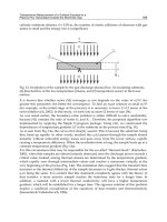
2.5.1 Thermocouple layout

According to the helical contact characteristics, eight thermocouples with the diameter of
0.3mm were embedded in the friction lining which are close to the contact surface. The
position of thermocouple is shown in Fig. 6. Firstly, the holes with the diameter of 1mm
were drilled on the lateral side of friction lining. Then the oddment of the friction lining was
filled in the hole after the thermocouple was embedded. In Fig. 8, points a, b and c were in
the central line of rope groove, points d and h were in the middle of contact zone I, points e
and f were in the middle of contact zone II and point g was in the middle of contact zone III.
The distance from points c, d, f, g and h to the contact surface is about 2mm, and the
distance between points e and f, a and b, b and c is about 2mm, too.


Fig. 6. Layout of thermocouple
2.5.2 Experimental parameters
The sliding speed and the equivalent pressure are the main factors affecting the
temperature rise of friction lining during the sliding process. Therefore, the experiments
were carried out with different sliding speeds and equivalent pressures. The sliding
distance is about 20m. According to the friction experiment standard for friction lining
(MT/T 248-91, 1991), the equivalent pressure is 1.5~3MPa. The parameters for the
experiment are listed in Table 1.

Heat Transfer – Engineering Applications

240

v≤10mm/s
v
＞10mm/s
Equivalent pressure (MPa) 1.5, 2, 2.5, 3 1.5, 2.5
Speed (mm/s) 1, 3, 5, 7, 10 30, 100, 300, 500, 700, 1000
Table 1. Parameters for friction experiment

2.5.3 Experimental results
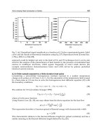
Fig. 7 shows the partial experiment results within the speed range of 1~10mm/s.


(a) 1mm/s (b) 7mm/s
Fig. 7. Variation of testing points' temperature
As shown in Fig. 7, the temperature rise is less than 5°C within 1 hour when the sliding
speed is less than 10mm/s. Therefore, the temperature rise of friction lining can be neglected
under the normal hoist condition. It is observed that the temperature increases wavily and
the amplitude of waveform increases with the sliding speed. This is due to the periodical
heat-flow resulting from the helical contact characteristics. In addition, the temperature
difference among 8 points is small and it increases with the equivalent pressure: the
temperature difference increases from 0.5°C to 2°C when the equivalent pressure increases
to 3MPa. It is found that the temperature increases quickly at the beginning of the sliding
process, and then it increases slowly.
In order to analyze the effect of the sliding speed and the equivalent pressure on the
temperature, Fig. 8 shows the temperature rise of point c at different sliding speeds and
equivalent pressures.
It is seen from Fig. 8 that the sliding speed has stronger effect than the equivalent pressure
on the temperature. It is concluded that the sliding speed is more sensitive to the
temperature. Therefore, only two equivalent pressures (1.5MPa and 2.5MPa) are selected at
the high-speed experiment.

Heat Conduction for Helical and Periodical Contact in a Mine Hoist

241


Fig. 8. Effect of speed and equivalent pressure on temperature within low speed

Fig. 9. Variation of testing points' temperature

Heat Transfer – Engineering Applications

242
As show in Fig. 9, the highest temperature rise increases to 15°C at the speed of 30mm/s.
Additionally, it is observed that the temperature at points c, d and f is higher than that at
other points. However, the temperature rise is not high enough to tell the highest among
them.


Distance between points and point to friction surface / mm (fs-friction surface)
a-b b-c c-fs d-fs e-f f-fs g-fs h-fs
1.5Mpa 2 2 1.8 1.38 2 2.16 2.24 2.24
2.5MPa 1.98 2.06 1.7 2 1.9 1.7 1.48 1.48
Table 2. Position of testing points in friction lining
In order to master the surface temperature of friction lining, the friction experiment was
performed with the increasing speed. Table 2 shows the distance of 8 points, and Fig. 10
shows the partial experiment results within the speed range 100~1000mm/s.
It is seen from Fig. 10 that the temperature rise of every point increases obviously. And the
order of temperature rise at testing points is shown in Table 3.

Pressure / speed
Order of temperature rise
Lining G
（high→low）
1.5MPa / 100mm/s d, c, f, b, e, a, g, h
1.5MPa / 400mm/s d, c, f, b, e, h, g, a
1.5MPa / 600mm/s d, f, c, g, h, e, b, a

1.5MPa / 800mm/s d, c, f, g, e, h, b, a
1.5MPa / 1000mm/s d, f, c, g, h, e, b, a
2.5MPa / 200mm/s f, g, c, d, e, h, b, a
2.5MPa / 300mm/s f, c, g, d, e, h, b, a
2.5MPa / 550mm/s f, c, g, d, e, h, b, a
2.5MPa / 750mm/s f, g, c, d, h, e, b, a
2.5MPa / 980mm/s f, c, d, g, h, e, b, a
Table 3. Order of temperature rise at testing points
The highest temperature rise occurs at point d with p
a
=1.5MPa while the highest
temperature rise appears at point f with p
a
=2.5MPa. This is because that point d is close to
the friction surface with the minimize distance of 1.38mm while the distance from point f to
friction surface is 2.16mm, which reveals the temperature gradient in the surface layer is
high. Therefore, the temperature at point d is higher than that at point f. It is found from
Table 3 that the temperature at points f, d and c is higher than that at other points, which is
in accordance with the analytical results of the helical contact characteristics and partial
heat-flow density. As shown in Fig. 3(b), the contact zone II is subject to the long-time heat-
flow and the convection heat transfer of contact zone I at the bottom of the rope groove is
worse than that of other zone. Consequently, the temperature at points c, d and f is higher.

Heat Conduction for Helical and Periodical Contact in a Mine Hoist

243

(a) 100-210mm/s (b) 300-400mm/s




(c) 550-600mm/s (d) 750-800mm/s

Heat Transfer – Engineering Applications

244




(e) 980-1000mm/s
Fig. 10. Variation of testing points' temperature


Fig. 11. Variation of temperature rise at point f with speed

Heat Conduction for Helical and Periodical Contact in a Mine Hoist

245
The variation of the temperature at point f with the speed is shown in Fig. 11. It is found that
the temperature at point f increases with the sliding speed. And the gradient of the
temperature rise increases rapidly with the speed at the beginning of the sliding process.
Additionally, from the drawing of partial enlargement 550mm/s, the temperature increases
periodically which agrees with the helical contact characteristics.
Combining Fig. 10 and Fig. 11, it is found that the temperature rise increases wavily at the

initial sliding stage, and the amplitude of wave increases with the sliding speed while it
decreases with the time. The explanation for the reduced temperature in the wavy temperature
is given as: (a) the rapid temperature rise results in decrease of the mechanical property, and
the contact area is enlarged which accelerates the heat exchange between friction lining and
wire rope, thus the temperature of friction lining reduces; (b) the increase of contact area
reduces the equivalent pressure and the heat-flow decreases rapidly; (c) due to unstable and
discontinuous speed at the initial sliding stage, the heat exchange between friction lining and
wire rope increases and the temperature decreases in a short time. As the sliding distance
increases, the heat exchange tends to balance which decrease the amplitude of the wave.
2.6 Analysis on numerical simulation and experimental results
In order to validate the theoretical model, the theoretical results are compared with the
experiment results. The parameters for the experiment are: v=0.55m/s, p
a
=2.5MPa.
h
1
=h
2
=h
4
=10W/m
2
K. Supposed that the contact surface of rope groove is only subjected to
heat-flow, then h
3
=0. r
1
=0.014m, r
2
=0.04m and T

0
=30°C. And the thermophysical properties
of wire rope are shown in Table 4.



w
/ (kgm
-3)
C
p
w
/ (Jkg
-1
K
-1
)

w
/ (Wm
-1
K
-1
)
Wire rope 7866 473 53.2
Table 4. Thermophysical properties of wire rope


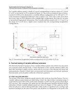
Fig. 12. Comparison between simulation and experimental results
As shown in Fig. 12, the temperature rise at point f increases to 52°C at 60s. From the

drawing of the partial enlargement at point f, the simulation result shows that the

Heat Transfer – Engineering Applications

246
temperature increases during the cycle of heat absorption and heat dissipation, which agrees
with the experiment results in Fig. 11. At the beginning of the sliding process, the
temperature of simulation result is higher than that of experiment results. And the
experimental value fluctuates obviously. This is because that the thermocouple absorbs the
heat, and the speed at the initial state of sliding process is unstable which leads to the heat
conduction for longer time at the local zone. Thus the experimental data is low and the
curve of temperature behaves serrasoidal. As the sliding process continues, the
experimental value is higher than the simulation value and the both values tend to be equal
in the end. This is because that the friction lining is subjected to temperature and stress and
the temperature rise results in the increase of surface deformation in the rope groove, which
makes the embedding thermocouple closer to the friction surface and leads to the rapid
temperature rise of the measuring point. Therefore, the experimental value is higher than
the theoretical value: the higher temperature rise at point f makes the deformation bigger
and the thermocouple is closer to the surface, which makes the temperature difference
between the experimental value and theoretical value at point f is higher than that at point
d. When the heat conduction tends to achieve the balance, the temperature variation gets
gently and the experimental value is consistent with the theoretical value. Compared the
experimental value with the theoretical value in Fig. 12, both of them agree well with each
other which validates the theoretical model of the temperature field.
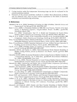
The above analysis indicates that the theoretical model of temperature field is reasonable and
correct. Due to difficultly obtaining the temperature of the friction surface by the way of the
direct contact measurement, the temperature of the contact surface is simulated in Fig. 13.
As in Fig. 13, the temperature on the friction surface is much higher: though the distance
between point f and friction surface is only 2mm, the temperature at friction surface is 18°C
higher than that at point f. In addition, the radial temperature gradient at different time is

simulated in Fig. 14. The temperature gradient at the surface layer is high and its maximum
is about 35000°C/m. And the temperature gradient decreases with the radius. As the sliding
process continues, the curve of temperature gradient at the surface layer tends to be flat. The


Fig. 13. Variation of temperature on friction surface

Heat Conduction for Helical and Periodical Contact in a Mine Hoist

247
above analysis indicates that the heat-conducting property of friction lining is poor. Thus, in
order to develop the new friction lining with good thermophysical properties, it is necessary
to optimize the ratio of basic material and filler and select the component with good heat-
conducting property.





Fig. 14. Radial temperature gradient at different time
3. Heat conduction for periodical contact
3.1 Theoretical model
As shown in Fig. 1, the disc brake for mine hoist is composed of brake disc and brake shoes.
During the braking process, the brake shoes are pushed onto the disc with a certain
pressure, and the friction force generated between them is applied to brake the drum of
mine hoist.
The heat energy caused by the friction between brake shoes and brake disc leads to their
temperature rise. However, the two important parts have different behaviors of heat
conduction: the brake shoe is subjected to continuous heat while the brake disc is heated
periodically due to rotational motion. And the two types of temperature field will be

discussed as follows.
3.1.1 Dynamic thermophysical properties of brake shoe
In order to obtain the temperature field of disc brake, it is necessary to obtain their
thermophysical properties. As the brake shoe is a kind of composite material, its dynamic
thermophysical properties (DTP) (specific heat capacity c
s
, thermal diffusivity a
s
and thermal
conductivity l
s
) vary with the temperature. And the testing results

(Bao, 2009) are shown in
Fig. 15.

Heat Transfer – Engineering Applications

248


50 100 150 200 250 300
6.0x10
-7
7.0x10
-7
8.0x10
-7
9.0x10
-7

1.0x10
-6
1.4
1.5
1.6
1.7
1000
1100
1200
1300
1400


s

s
/ m
2
·s
-1
T
/ ℃


s


s
/ W·m
-1

·K
-1
c
s
c
s
/ J·kg
-1
·K
-1


Fig. 15. Dynamic thermophysical properties of brake shoe
According to the data in Fig. 15, the fitting equations of DTP are gained by regression
analysis

30
153.843
-3 -5 2 -7 3 -10 4
-3 -5 2 -7 3 -10 4
0.509 ,
=1.694+1.21 10 -3 10 +1.436 10 -2.144 10 ,
0.864+5.59 10 -4 10 +1.56 10 -2.3 10 .
T
s
s
s
e
TT T T
cTTTT






  
 
(16)
The brake disc is a kind of steel material, and it is generally assumed that its thermophysical
properties are invariable during the braking process. And its static thermophysical
parameters (STP) are shown in Table 5.


d
[kgm
-3
] c
d
[Jkg
-1
K
-1
]

d
 [Wm
-1
K
-1
]

7866 473 53.2
Table 5. Static thermophysical parameters of brake disc
Accordingly, the dynamic distribution coefficient of heat-flux is obtained (Zhu, 2009):

1
,
1
1,
s
dd d
ss s
ds
k
c
c
kk







(17)
where k
s
and k
d
are the dynamic distribution coefficient of heat-flux for brake shoe and
brake disc, respectively.

Combining Eq. (16) and Eq. (17), the dynamic distribution coefficient of heat-flux is plotted
in Fig. 16. The curves show that the distribution coefficient of heat-flux for the brake disc
always exceeds 0.88, and it absorbs most of heat energy. And k
d
decreases with the
temperature until 270°C, then it increases above 270°C. According to Eq. (17), k
s
has the
reverse variation.

Heat Conduction for Helical and Periodical Contact in a Mine Hoist

249
30 60 90 120 150 180 210 240 270 300
0.10
0.11
0.12
0.13
0.14
0.15
0.85
0.86
0.87
0.88
0.89
0.90
k
s
k
s

T / ℃
k
d

k
d

Fig. 16. Dynamic distribution coefficient of heat-flux
3.1.2 Partial differential equation of heat conduction
As shown in Fig. 17, the cylindrical coordinate is used to describe their geometry. Based on
the theory of heat conduction, the transient models of disc brake’s temperature field are as
follows:

2
11
,
ss ss
ss ss s s
ssssss
s
TT TT
cr
trt r z z
r
 

 
 

 

 
 
 
(18)

22
22 2
11
.
dd d d d d
ddd
dd d
cT T T T
r
trt r
rz











(19)

Fig. 17. Geometry Model of disc brake
3.1.3 Heat-flux
Suppose that the friction heat energy is absorbed completely by the brake shoe and brake
disc

,
, ,
ds
ddss
qq q
q
k
qq
k
q


(20)

Heat Transfer – Engineering Applications

250
where q is the whole heat-flux, q
d
and q
s
are the disc’s and shoe’s heat-flux, respectively.
And the












,,
q
rt
fp
tvt
fp
ttr


  (21)
where f is the coefficient of friction between brake disc and brake shoe, p is the brake
pressure, v and w are the linear and angular velocity. The brake pressure pushed onto the
brake disc increases gradually, and the pressure is given as

(Cao & Lin, 2002)


0
1,
z
t

t
pt p e






(22)
where p
0
is the initial brake pressure, and t
z
is total braking time. In addition, the angular
velocity is assumed to decrease linearly, then

0
1,
z
t
t





(23)
where
000
vr



, v
0
is the initial linear velocity and r
0
is the average radius.
Combining Eq.(21), Eq.(22) and Eq.(23), the whole heat-flux is gained as following


00
,11.
z
t
t
z
t
qrt f p e r
t






   





(24)
3.1.4 Boundary conditions
During the barking process, the brake disc rotates while the brake shoe keeps static.
Therefore, the brake disc and brake shoe have different boundary conditions. For the brake
shoe, its friction surface is subjected to the constant heat-flux.



12
,,,0,,0.
sf s s z s
qqrrrt tz

 
(25)
With regard to the fixed area in the brake disc, it is subject to the periodical heat-flux. In
order to calculate the temperature rise of brake disc, the movable heat-flux is expressed by




1010 12
2
10
0
, , , , , 0
d.
2
df d d d d
t

z
qq rrrz
t
tt t
t

 

   






(26)
where
11 1
2 π, mod2πnn


  .
3.2 Results and discussion
According to the above theory analysis, the temperature rise of brake shoe and brake disc is
simulated by finite element method. The dimension parameters are as follows:
1
2.35r 
,

Heat Conduction for Helical and Periodical Contact in a Mine Hoist

251
2
2.55r  ,


012
2rrr
,


0,2π
d


,
0
0.0612

 ,


0.03,0
d
r 
,


0,0.025
s

r 
. The
braking parameters are shown in Table 6. And Figs. 18-23 show the simulation results.

f
p [MPa]
v
0
[ms
-1
]
t
z
[s]
0.4 1.36 10 7.32
Table 6. Braking parameters for disc brake



012345678
20
40
60
80
100
120
140
160
180
T

s
/
℃
t / s
r
s
= 2.45,

s

z
s
= 0
012345678
20
22
24
26
28
30
32
T
d
/ ℃
t / s
r
d
= 2.45,

d


/3, z
d
= 0


Fig. 18. Temperature rise of disc brake



2.35
2.40
2.45
2.50
2.55
0.0
2.0x10
5
4.0x10
5
6.0x10
5
8.0x10
5
1.0x10
6
1.2x10
6
0
1

2
3
4
5
6
7
q

/

W
·
m
-
2
t

/

s
r

/

m


Fig. 19. Variation of heat-flux with t and r

Heat Transfer – Engineering Applications

252
It is seen from Fig. 18 that DTP has little effect on the temperature rise. The brake shoe’s
temperature calculated with DTP is a little higher than that with STP, while the temperature
of brake disc with DTP is in accordance with that with STP. In Fig. 18, the temperature of
brake shoe varies smoothly while the temperature of brake disc changes periodically. In Fig.
18(a), the temperature of brake shoe increases with the time and reaches the maximum
169°C at t = 5.3s, then it decreases. This result agrees with the variation of heat-flux in Fig.
19: there is a peak in the curve of heat-flux during the braking process. Though the brake
disc absorbs most of friction heat, its maximal temperature, which is only 30°C, is much
lower than brake shoe's. With regard to the fixed point in brake disc, it is subject to heat-flux
within short time and convects with the air in most time of every circle. Thus, the
temperature of brake disc is lower and varies periodically.
In addition, the temperature of fixed point at different q
d
in a circle is simulated, and the
simulation results are in Fig. 20. The peak of temperature occurs when the point on the disc
contacts with the shoe. And the variation of temperature peak agrees well with the variation
of heat-flux during the braking process. Furthermore, the variation of temperature with
radius is shown in Fig. 21. The temperature of brake shoe increases with the radius slightly
for minor difference between inner and outer radius. The temperature on both edges of the
contact zone in brake disc is low, while it is high in the middle.

012345678
20
22
24
26
28
30
32
T
d
/ ℃
t / s


d
= /3


d
= /3


d
= 


d
= /3



d
= /3
r
d
= 2.45, z
d
= 0





Fig. 20. Variation of T
d
with q
d

Heat Conduction for Helical and Periodical Contact in a Mine Hoist

253
2.35 2.40 2.45 2.50 2.55
20
40
60
80
100
120
140
160
180


s
= , z
s
= 0
T
s
/ ℃
r
s
/ m
t = 1s
t = 2s
t = 3s
t = 4s
t = 5s
t = 6s
t = 7s

(a) brake shoe
2.35 2.40 2.45 2.50 2.55
20
21
22
23
24
25
t = 1s
t = 2s
t = 3s

t = 4s
t = 5s
t = 6s
t = 7s
T
d
/ ℃
r
d
/ m

d
= /2, z
d
= 0

(b) brake disc
Fig. 21. Variation of temperature with radius

0.000 0.005 0.010 0.015 0.020 0.025
20
40
60
80
100
120
140
160
180
T

s
/ ℃
z
s
/ m
t = 1s
t = 2s
t = 3s
t = 4s
r
s
= 2.45,

s
= 0
0.00 -0.01 -0.02 -0.03
20
21
22
23
T
d
/ ℃
z
d
/ m
t = 1s
t = 2s
t = 3s
t = 4s

r
d
= 2.45,

d
= /2

(a) brake shoe (b) brake disc
Fig. 22. Variation of temperature with depth