Hydrodynamics Advanced Topics Part 1 docx
Bạn đang xem bản rút gọn của tài liệu. Xem và tải ngay bản đầy đủ của tài liệu tại đây (790.21 KB, 30 trang )
HYDRODYNAMICS –
ADVANCED TOPICS
Edited by Harry Edmar Schulz,
André Luiz Andrade Simões
and Raquel Jahara Lobosco
Hydrodynamics – Advanced Topics
Edited by Harry Edmar Schulz, André Luiz Andrade Simões and Raquel Jahara Lobosco
Published by InTech
Janeza Trdine 9, 51000 Rijeka, Croatia
Copyright © 2011 InTech
All chapters are Open Access distributed under the Creative Commons Attribution 3.0
license, which allows users to download, copy and build upon published articles even for
commercial purposes, as long as the author and publisher are properly credited, which
ensures maximum dissemination and a wider impact of our publications. After this work
has been published by InTech, authors have the right to republish it, in whole or part, in
any publication of which they are the author, and to make other personal use of the
work. Any republication, referencing or personal use of the work must explicitly identify
the original source.
As for readers, this license allows users to download, copy and build upon published
chapters even for commercial purposes, as long as the author and publisher are properly
credited, which ensures maximum dissemination and a wider impact of our publications.
Notice
Statements and opinions expressed in the chapters are these of the individual contributors
and not necessarily those of the editors or publisher. No responsibility is accepted for the
accuracy of information contained in the published chapters. The publisher assumes no
responsibility for any damage or injury to persons or property arising out of the use of any
materials, instructions, methods or ideas contained in the book.
Publishing Process Manager Bojana Zelenika
Technical Editor Teodora Smiljanic
Cover Designer InTech Design Team
Image Copyright André Luiz Andrade Simões, 2011.
First published December, 2011
Printed in Croatia
A free online edition of this book is available at www.intechopen.com
Additional hard copies can be obtained from
Hydrodynamics – Advanced Topics,
Edited by Harry Edmar Schulz, André Luiz Andrade Simões and Raquel Jahara Lobosco
p. cm.
ISBN 978-953-307-596-9
free online editions of InTech
Books and Journals can be found at
www.intechopen.com
Contents
Preface IX
Part 1 Mathematical Models in Fluid Mechanics 1
Chapter 1 One Dimensional Turbulent
Transfer Using Random Square Waves –
Scalar/Velocity and Velocity/Velocity Interactions 3
H. E. Schulz, G. B. Lopes Júnior,
A. L. A. Simões and R. J. Lobosco
Chapter 2 Generalized Variational Principle
for Dissipative Hydrodynamics:
Shear Viscosity from Angular
Momentum Relaxation in the
Hydrodynamical Description of Continuum Mechanics 35
German A. Maximov
Chapter 3 Nonautonomous Solitons:
Applications from Nonlinear Optics
to BEC and Hydrodynamics 51
T. L. Belyaeva
and V. N. Serkin
Chapter 4 Planar Stokes Flows with Free Boundary 77
Sergey Chivilikhin and Alexey Amosov
Part 2 Biological Applications and Biohydrodynamics 93
Chapter 5 Laser-Induced Hydrodynamics in
Water and Biotissues Nearby Optical Fiber Tip 95
V. I. Yusupov, V. M. Chudnovskii and V. N. Bagratashvili
Chapter 6 Endocrine Delivery System of NK4, an
HGF-Antagonist and Anti-Angiogenic Regulator, for
Inhibitions of Tumor Growth, Invasion and Metastasis 119
Shinya Mizuno and Toshikazu Nakamura
VI Contents
Part 3 Detailed Experimental Analyses of Fluids and Flows 143
Chapter 7 Microrheology of Complex Fluids 145
Laura J. Bonales,
Armando Maestro,
Ramón G. Rubio and Francisco Ortega
Chapter 8 Hydrodynamics Influence on
Particles Formation Using SAS Process 169
A. Montes, A. Tenorio, M. D. Gordillo,
C. Pereyra and E. J. Martinez de la Ossa
Chapter 9 Rotational Dynamics of Nonpolar
and Dipolar Molecules in Polar
and Binary Solvent Mixtures 185
Sanjeev R. Inamdar
Chapter 10 Flow Instabilities in
Mechanically Agitated Stirred Vessels 227
Chiara Galletti and Elisabetta Brunazzi
Chapter 11 Hydrodynamic Properties of
Aggregates with Complex Structure 251
Lech Gmachowski
Part 4 Radiation-, Electro-,
Magnetohydrodynamics and Magnetorheology 267
Chapter 12 Electro-Hydrodynamics of
Micro-Discharges in Gases
at Atmospheric Pressure 269
O. Eichwald, M. Yousfi, O. Ducasse,
N. Merbahi, J.P. Sarrette, M. Meziane and M. Benhenni
Chapter 13 An IMEX Method for the Euler Equations that
Posses Strong Non-Linear Heat Conduction and
Stiff Source Terms (Radiation Hydrodynamics) 293
Samet Y. Kadioglu
and Dana A. Knoll
Chapter 14 Hydrodynamics on Charged Superparamagnetic
Microparticles in Water Suspension:
Effects of Low-Confinement
Conditions and Electrostatics Interactions 319
P. Domínguez-García
and M.A. Rubio
Chapter 15 Magnetohydrodynamics of Metallic Foil
Electrical Explosion and Magnetically
Driven Quasi-Isentropic Compression 347
Guiji Wang, Jianheng Zhao, Binqiang Luo and Jihao Jiang
Contents VII
Part 5 Special Topics on Simulations and Experimental Data 379
Chapter 16 Hydrodynamics of a Droplet in Space 381
Hitoshi Miura
Chapter 17 Flow Evolution Mechanisms of Lid-Driven Cavities 411
José Rafael Toro and Sergio Pedraza R.
Chapter 18 Elasto-Hydrodynamics of
Quasicrystals and Its Applications 429
Tian You Fan and Zhi Yi Tang
Preface
“Water is the beginning of everything” (Tales of Mile to)
“Air is the beginning of everything” (Anaxagoras of Mile to)
Introduction
Why is it important to study Hydrodynamics? The answer may be strictly technical,
but it may also involve some kind of human feeling about our environment and our
(eventual) limitations to deal with its fluidic constituents.
As teachers, when talking to our students about the importance of quantifying fluids,
we (authors) go to the blackboard and draw, in blue color, a small circumference in the
center of the board, and add the obvious name 'Earth'. Some words are then said, in
the sense that Hydrodynamics is important, because we are beings strictly adapted to
live immersed in a fluidic environment (air), and because we are beings composed
basically by simple fluidic solutions (water solutions), encapsulated in fine carbon
membranes. Then, with a red chalk, we draw two crosses: one inside and the other
outside the circumference, explaining: “our environment is very limited. We can only
survive in the space covered by the blue line. No one of us can survive in the inner
part of this sphere, or in the outer space. Despite all films, games, and books about
contacts with aliens, and endless journeys across the universe, our present knowledge
only allows to suggest that it is most probable that the human being will extinct while
in this fine fluid membrane, than to create sustainable artificial environments in the
cosmos”.
Sometimes, to add some drama, we project the known image of the earth on a wall
(the image of the blue sphere), and then we blow a soap bubble explaining that the
image gives the false impression that the entire sphere is our home. But our “home” is
better represented by the liquid film of the soap bubble (only the film) and then we
touch the bubble, exploding it, showing its fragility.
In the sequence, we explain that a first reason to understand fluids would be, then, to
guarantee the maintenance of the fluidic environment (the film) so that we could also
guarantee our survival as much as possible. Further, as we move ourselves and
produce our things immersed in fluid, it is interesting to optimize such operations in
order to facilitate our survival. Still further, because our organisms interchange heat
X Preface
and mass in cellular and corporal scales between different fluids, the understanding of
these transports permits us to understand the spreading of diseases, the delivering of
medicines to cells, and the use of physical properties of fluids in internal treatments.
Thus, understanding these transports allows us to improve our quality of life. Finally,
the observation of the inner part of the sphere, the outer space and its constituents,
shows that many “highly energetic” phenomena behave like the fluids around us. It
gives us the hope that the knowledge of fluids can help, in the future, to quantify,
reproduce, control and use energy sources similar to those of the stars, allowing us to
“move through the cosmos”, to create sustainable artificial environments and to leave
this “limited film” when necessary. Of course, this “speech” may be viewed as a sort
of escapism, related to a fiction of the future. In fact, the day-by-day activities show
that we are spending our time with “more important” things, like fighting among us
for the dividends of the next fashion wave (or the next technical wave), the hierarchy
among nations, or the hierarchy of the cultures of the different nations. So, fighters,
warriors, or generals still seem to be the agents that write our history. But global
survival, or, in other words, the guarantee of any future history, will need other
agents, devoted to other activities. The hope lies on the generation of knowledge, in
which the knowledge about fluids is vital.
Context of the present book “Hydrodynamics - Advanced Topics”
A quick search in virtual book stores may result in more than one hundred titles
involving the word “Hydrodynamics”. Considering the superposition existing with
Fluid Mechanics, the number of titles grows much more. Considering all these titles,
why try to organize another book on Hydrodynamics? One answer could be that the
researchers always try new points of view to understand and treat the problems
related to Hydrodynamics. Even a much known phenomenon may be re-explained
from a point of view that introduces different tools (conceptual, numerical or practical)
into the discussion of fluids. And eventually, a detail shows to be useful, or even very
relevant. So, it is necessary to give the opportunity for the different authors to expose
their points of view.
Among the historically relevant books on Hydrodynamics, some should be mentioned
here. For example, the volumes “Hydrodynamics” and “Hydraulics”, by Daniel
Bernoulli (1738) and his father, Johann Bernoulli (1743) present many interesting
sketches and the analyses that converged to the so called “Bernoulli equation”, later
deduced more properly by Leonhard Euler. Although there are unpleasant questions
about the authorship of the main ideas, as pointed out by Rouse (1967) and Calero
(2008), both books are placed in a “prominent position” in history, because of their
significant contributions. The volume written by Sir Horace Lamb (1879), now named
“Hydrodynamics”, considers the basic equations, the vortex motion, and tidal waves,
among other interesting topics. Considering the classical equations and procedures
followed to study fluid motion, the books “Fundamentals of Hydro and
Aerodynamics“ and “Applied Hydro and Aerodynamics“ by Prandtl and Tietjens
(1934) present the theory and its practical applications in a comprehensive way,
Preface XI
influencing the experimental procedures for several decades. For over fifty years, the
classical volume of Landau and Lifschitz (1959) remains an extremely valuable work
for researchers in fluid mechanics.
In addition to the usual themes, like the basic equations and turbulence, this book also
covers themes like the relativistic fluid dynamics and the dynamics of superfluids. Each
of the major topics considered in the studies of fluid mechanics can be widely discussed,
generating specific texts and books. An example is the theory of boundary layers, in
which the book of Schlichting (1951) has been considered an indispensable reference,
because it condenses most of the basic concepts on this subject. Further, still considering
specific topics, Stoker (1957) and Lighthill (1978) wrote about waves in fluids, while
Chandrasekhar (1961) and Drazin and Reid (1981) considered hydrodynamic and
hydromagnetic stability. It is also necessary to mention the books of Batchelor (1953),
Hinze (1958), and Monin and Yaglom (1965), which are notable examples of texts on
turbulence and statistical fluid mechanics, showing basic concepts and comparative
studies between theory and experimental data. A more recent example may be the
volume written by Kundu e Cohen (2008), which furnishes a chapter on “biofluid
mechanics” The list of the “relevant books” is obviously not complete, and grows
continuously, because new ideas are continuously added to the existing knowledge.
The present book is one of the results of a project that generated three volumes, in
which recent studies on Hydrodynamics are described. The remaining two titles are
“Hydrodynamics - Natural Water Bodies”, and “Hydrodynamics - Optimizing
Methods and Tools”. Along the chapters of the present volume, the authors show the
application of concepts of Hydrodynamics in different fields, using different points of
view and methods. The editors thank all authors for their efforts in presenting their
chapters and conclusions, and hope that this effort will be welcomed by the
professionals working with Hydrodynamics.
The book “Hydrodynamics - Advanced Topics” is organized in the following manner:
Part 1: Mathematical Models in Fluid Mechanics
Part 2: Biological Applications and Biohydrodynamics
Part 3: Detailed Experimental Analyses of Fluids and Flows
Part 4: Radiation-, Electro-, Magnetohydrodynamics and Magnetorheology
Part 5: Special Topics on Simulations and Experimental Data
Hydrodynamics is a very rich area of study, involving some of the most intriguing
theoretical problems, considering our present level of knowledge. General nonlinear
solutions, closed statistical equations, explanation of sudden changes, for example, are
wanted in different areas of research, being also a matter of study in Hydromechanics.
Further, any solution in this field depends on many factors, or many “boundary
conditions”. The changing of the boundary conditions is one of the ways through
which the human being affects its fluidic environment. Changes in a specific site can
impose catastrophic consequences in a whole region. For example, the permanent
leakage of petroleum in one point in the ocean may affect the life along the entire
XII Preface
region covered by the marine currents that transport this oil. Gases or liquids, the
changes in the quality of the fluids in which we live, certainly affect our quality of life.
The knowledge about fluids, their movements, and their ability to transport physical
properties and compounds is thus recognized as important for life. As a consequence,
thinking about new solutions for general or specific problems in Hydromechanics may
help to attain a sustainable relationship with our environment. Re-contextualizing the
classical discussion about the truth, in which it was suggested that the “thinking” is
the guarantee of our “existence” (St. Augustine, 386a, b, 400), we can say that we agree
that thinking guarantees the human existence, and that there are too many warriors,
and too few thinkers. Following this re-contextualized sense, it was also said that the
man is a bridge between the “animal” and “something beyond the man” (Nietzsche,
1883). This is an interesting metaphor, because bridges are built crossing fluids (even
abysms are filled with fluids). Considering all possible interpretations of this phrase,
let us study and understand the fluids, and let us help to build the bridge.
Dr. Harry Edmar Schulz
Nucleus of Thermal Engineering and Fluids,
Department of Hydraulics and Sanitary Engineering,
School of engineering at Sao Carlos,
University of Sao Paulo,
Brazil
Dr. Andre Luiz Andrade Simoes
Laboratory of Turbulence and Rheology,
Department of Hydraulics and Sanitary Engineering,
School of engineering at Sao Carlos,
University of Sao Paulo,
Brazil
Dr. Raquel Jahara Lobosco
Laboratory of Turbulence and Rheology,
Department of Hydraulics and Sanitary Engineering,
School of engineering at Sao Carlos,
University of Sao Paulo,
Brazil
References
Batchelor, G.K. (1953), The theory of homogeneous turbulence. First published in the
Cambridge Monographs on Mechanics and Applied Mathematics series 1953.
Reissued in the Cambridge Science Classics series 1982 (ISBN: 0 521 04117 1).
Bernoulli, D. (1738), Hydrodynamics. Dover Publications, Inc., Mineola, New York,
1968 (first publication) and reissued in 2005, ISBN-10: 0486441857.
Preface XIII
Hydrodynamica, by Daniel Bernoulli, as published by Johann Reinhold
Dulsecker at Strassburg in 1738.
Bernoulli, J. (1743), Hydraulics. Dover Publications, Inc., Mineola, New York, 1968
(first publication) and reissued in 2005, ISBN-10: 0486441857. Hydraulica, by
Johann Bernoulli, as published by Marc-Michel Bousquet et Cie. at Lausanne
and Geneva in 1743.
Calero, J.S. (2008), The genesis of fluid mechanics (1640-1780). Springer, ISBN 978-1-
4020-6413-5. Original title: La génesis de la Mecánica de los Fluidos (1640–
1780), UNED, Madrid, 1996.
Chandrasekhar, S. (1961), Hydrodynamic and Hydromagnetic Stability. Clarendon
Press edition, 1961. Dover edition, first published in 1981 (ISBN: 0-486-64071-
X).
Drazin, P.G. & Reid, W.H. (1981), Hydrodynamic stability. Cambridge University
Press (second edition 2004). (ISBN: 0 521 52541 1).
Hinze, J.O. (1959), Turbulence. McGraw-Hill, Inc. second edition, 1975 (ISBN:0-07-
029037-7).
Kundu, P.K. & Cohen, I.M. (2008), Fluid Mechanics. 4
th
ed. With contributions by P.S.
Ayyaswamy and H.H. Hu. Elsevier/Academic Press (ISBN 978-0-12-373735-
9).
Lamb, H. (1879), Hydrodynamics (Regarded as the sixth edition of a Treatise on the
Mathematical Theory of the Motion of Fluids, published in 1879). Dover
Publications, New York., sixth edition, 1993 (ISBN-10: 0486602567).
Landau, L.D.; Lifschitz, E.M. (1959), Fluid Mechanics. Course of theoretical Physics,
Volume 6. Second edition 1987 (Reprint with corrections 2006). Elsevier
(ISBN-10: 0750627670).
Lighthill, J. (1978), Waves in Fluids. Cambridge University Press, Reissued in the
Cambridge Mathematical Library series 2001, Third printing 2005 (ISBN-10:
0521010454).
Monin, A.S. & Yaglom, A.M. (1965), Statistical fluid mechanics: mechanics of
turbulence. Originally published in 1965 by Nauka Press, Moscow, under the
title Statisticheskaya Gidromekhanika-Mekhanika Turbulentnosti. Dover
edition, first published in 2007. Volume 1 and Volume 2.
St. Augustine (386a), Contra Academicos, in Abbagnano, N. (2007), Dictionary of
Philosophy, “Cogito”, Martins Fontes, Brasil (Text in Portuguese).
St. Augustine (386b), Soliloquia, in Abbagnano, N. (2007), Dictionary of Philosophy,
“Cogito”, Martins Fontes, Brasil (Text in Portuguese).
St. Augustine (400-416), De Trinitate, in Abbagnano, N. (2007), Dictionary of
Philosophy, “Cogito”, Martins Fontes, Brasil (Text in Portuguese).
Nietzsche, F. (1883), Also sprach Zarathustra, Publicações Europa-América, Portugal
(Text in Portuguese, Ed. 1978).
Rouse, H. (1967). Preface to the english translation of the books Hydrodynamics and
Hydraulics, already mentioned in this list. Dover Publications, Inc.
Prandtl, L. & Tietjens, O.G. (1934) Fundamentals of Hydro & Aeromechanics, Dover
Publications, Inc. Ed. 1957.
XIV Preface
Prandtl, L. & Tietjens, O.G. (1934) Applied Hydro & Aeromechanics, Dover
Publications, Inc. Ed. 1957.
Schlichting, H. (1951), Grenzschicht-Theorie. Karlsruhe: Verlag und Druck.
Stoker, J.J. (1957). Water waves: the mathematical theory with applications.
Interscience Publishers, New York (ISBN-10: 0471570346).
Part 1
Mathematical Models in Fluid Mechanics
1
One Dimensional Turbulent Transfer Using
Random Square Waves – Scalar/Velocity
and Velocity/Velocity Interactions
H. E. Schulz
1,2
, G. B. Lopes Júnior
2
, A. L. A. Simões
2
and R. J. Lobosco
2
1
Nucleus of Thermal Engineering and Fluids
2
Department of Hydraulics and Sanitary Engineering School
of Engineering of São Carlos, University of São Paulo
Brazil
1. Introduction
The mathematical treatment of phenomena that oscillate randomly in space and time,
generating the so called “statistical governing equations”, is still a difficult task for scientists
and engineers. Turbulence in fluids is an example of such phenomena, which has great
influence on the transport of physical proprieties by the fluids, but which statistical
quantification is still strongly based on ad hoc models. In turbulent flows, parameters like
velocity, temperature and mass concentration oscillate continuously in turbulent fluids, but
their detailed behavior, considering all the possible time and space scales, has been
considered difficult to be reproduced mathematically since the very beginning of the studies
on turbulence. So, statistical equations were proposed and refined by several authors,
aiming to describe the evolution of the “mean values” of the different parameters (see a
description, for example, in Monin & Yaglom, 1979, 1981).
The governing equations of fluid motion are nonlinear. This characteristic imposes that the
classical statistical description of turbulence, in which the oscillating parameters are
separated into mean functions and fluctuations, produces new unknown parameters when
applied on the original equations. The generation of new variables is known as the “closure
problem of statistical turbulence” and, in fact, appears in any phenomena of physical nature
that oscillates randomly and whose representation is expressed by nonlinear conservation
equations. The closure problem is described in many texts, like Hinze (1959), Monin &
Yaglom (1979, 1981), and Pope (2000), and a general form to overcome this difficulty is
matter of many studies.
As reported by Schulz et al. (2011a), considering scalar transport in turbulent fluids, an
early attempt to theoretically predict RMS profiles of the concentration fluctuations using
“ideal random signals” was proposed by Schulz (1985) and Schulz & Schulz (1991). The
authors used random square waves to represent concentration oscillations during mass
transfer across the air-water interface, and showed that the RMS profile of the
concentration fluctuations may be expressed as a function of the mean concentration
profile. In other words, the mean concentration profile helps to know the RMS profile. In
these studies, the authors did not consider the effect of diffusion, but argued that their
Hydrodynamics – Advanced Topics
4
equation furnished an upper limit for the normalized RMS value, which is not reached
when diffusion is taken into account.
The random square waves were also used by Schulz et al. (1991) to quantify the so called
“intensity of segregation” in the superficial boundary layer formed during mass transport,
for which the explanations of segregation scales found in Brodkey (1967) were used. The
time constant of the intensity of segregation, as defined in the classical studies of Corrsin
(1957, 1964), was used to correlate the mass transfer coefficient across the water surface with
more usual parameters, like the Schmidt number and the energy dissipation rate. Random
square waves were also applied by Janzen (2006), who used the techniques of Particle Image
Velocimetry (PIV) and Laser Induced Fluorescence (LIF) to study the mass transfer at the
air-water interface, and compared his measurements with the predictions of Schulz &
Schulz (1991) employing ad hoc concentration profiles. Further, Schulz & Janzen (2009)
confirmed the upper limit for the normalized RMS of the concentration fluctuations by
taking into account the effect of diffusion, also evaluating the thickness of diffusive layers
and the role of diffusive and turbulent transports in boundary layers. A more detailed
theoretical relationship for the RMS of the concentration fluctuation showed that several
different statistical profiles of turbulent mass transfer may be interrelated.
Intending to present the methodology in a more organized manner, Schulz et al. (2011a)
showed a way to “model” the records of velocity and mass concentration (that is, to
represent them in an a priori simplified form) for a problem of mass transport at gas-liquid
interfaces. The fluctuations of these variables were expressed through the so called
“partition, reduction, and superposition functions”, which were defined to simplify the
oscillating records. As a consequence, a finite number of basic parameters was used to
express all the statistical quantities of the equations of the problem in question. The
extension of this approximation to different Transport Phenomena equations is
demonstrated in the present study, in which the mentioned statistical functions are derived
for general scalar transport (called here “scalar-velocity interactions”). A first application for
velocity fields is also shown (called here “velocity-velocity interactions”). A useful
consequence of this methodology is that it allows to “close” the turbulence equations,
because the number of equations is bounded by the number of basic parameters used. In
this chapter we show 1) the a priori modeling (simplified representation) of the records of
turbulent variables, presenting the basic definitions used in the random square wave
approximation (following Schulz et al., 2011a); 2) the generation of the usual statistical
quantities considering the random square wave approximation (scalar-velocity interactions);
3) the application of the methodology to a one-dimensional scalar transport problem,
generating a closed set of equations easy to be solved with simple numerical resources; and
4) the extension of the study of Schulz & Johannes (2009) to velocity fields (velocity-velocity
interactions).
Because the method considers primarily the oscillatory records itself (a priori analysis), and
not phenomenological aspects related to physical peculiarities (a posteriori analysis, like the
definition of a turbulent viscosity and the use of turbulent kinetic energy and its dissipation
rate), it is applicable to any phenomenon with oscillatory characteristics.
2. Scalar-velocity interactions
2.1 Governing equations for transport of scalars: Unclosed statistical set
The turbulent transfer equations for a scalar F are usually expressed as
One Dimensional Turbulent Transfer
Using Random Square Waves – Scalar/Velocity and Velocity/Velocity Interactions
5
iFi
ii i
FF F
VDvf
g
txx x
, i = 1, 2, 3. (1)
where
F and f are the mean scalar function and the scalar fluctuation, respectively.
i
V
(i =
1, 2, 3) are mean velocities and v
i
are velocity fluctuations, t is the time, x
i
are the Cartesian
coordinates,
g
represents the scalar sources and sinks and D
F
is the diffusivity coefficient of
F. For one-dimensional transfer, without mean movements and generation/consumption of
F, equation (1) with x
3
=z and v
3
= is simplified to
F
FF
D ωf
tz z
(2)
As can be seen, a second variable, given by the mean product
ωf
, is added to the equation
of
F
, so that a second equation involving ωf and
F
is needed to obtain solutions for both
variables. Additional statistical equations may be generated averaging the product between
equation (1) and the instantaneous fluctuations elevated to some power (
f
). As any new
equation adds new unknown statistical products to the problem, the resulting system is
never closed, so that no complete solution is obtained following strictly statistical
procedures (closure problem). Studies on turbulence consider a low number of statistical
equations (involving only the first statistical moments), together with additional equations
based on
ad hoc models that close the systems. This procedure seems to be the most natural
choice, because having already obtained equation (2), it remains to model the new parcel
ω f
a posteriori (that is, introducing hypotheses and definitions to solve it). An example is
the combined use of the Boussinesq hypothesis (in which the turbulent viscosity/diffusivity
is defined) with the Komogoroff reasoning about the relevance of the turbulent kinetic
energy and its dissipation rate. The
− model for statistical turbulence is then obtained,
for which two new statistical equations are generated, one of them for k and the other for
.
Of course, new unknown parameters appear, but also additional ad hoc considerations are
made, relating them to already defined variables.
In the present chapter, as done by Schulz et al. (2011a), we do not limit the number of
statistical equations based on a posteriori definitions for
ω f
. Convenient a priori definitions
are used on the oscillatory records, obtaining transformed equations for equation (1) and
additional equations. The central moments of the scalar fluctuations,
f
FF
, = 1, 2,
3,… are considered here. For example, the one-dimensional equations for
=2, 3 and 4, are
given by
222
2
11
22
F
f
Ff f
fDf
tzz
z
(3a)
3322
22 2 2
22
11
33
F
f
FFf Ff
ff Df f
tt zz
zz
(3b)
Hydrodynamics – Advanced Topics
6
4422
33 3 3
22
11
44
F
f
FF
f
F
f
ff Df f
tt zz
zz
(3c)
In this example, equation (3a) involves
F and
f
of equation (2), but adds three new
unknowns. The first four equations (2) and (3 a, b, c) already involve eleven different
statistical quantities:
F
,
2
f
,
3
f
,
4
f
,
f
,
2
f
,
3
f
,
4
f
,
2
2
f
f
z
,
2
2
2
f
f
z
, and
2
3
2
f
f
z
, and the “closure” is not possible. The general equation for central moments, for
any
, is given by [20]
22
11 1 1
22
11
F
f
FF
f
F
f
ff Df f
tt zz
zz
(3d)
(using
=1 reproduces equation (2)).
As mentioned, the method models the records of the oscillatory variables, using random
square waves. The number of equations is limited by the number of the basic parameters
defined “
a priori”.
2.2 “Modeling” the records of the oscillatory variables
As mentioned in the introduction, the term “modeling” is used here as “representing in a
simplified way”. Following Schulz et al. (2011a), consider the function
F(z, t) shown in
Figure 1. It represents a region of a turbulent fluid in which the scalar quantity
F oscillates
between two functions
F
p
(p=previous) and F
n
(n=next) in the interval z
1
<z<z
2
. Turbulence is
assumed stationary.
Fig. 1a. A two-dimensional random scalar
field F oscillating between the boundary
functions
F
p
(t) and F
n
(t).
Fig. 1b. Sketch of the region shown in figure
(1a). Turbulence is stationary. Adapted from
Schulz et al. (2011a)
The time average of
F(z, t) for
12
zzz
, indicated by (,)Fzt is defined as usual
2
1
12
1
(,) (,)
t
t
Fzt Fztdt for z z z
t
(4)
One Dimensional Turbulent Transfer
Using Random Square Waves – Scalar/Velocity and Velocity/Velocity Interactions
7
21
tt t
is the time interval for the average operation. Equation (4) generates a mean
value
()Fz for
12
zzz
and
12
ttt
. Any statistical quantity present in equations 3, like,
for example, the central moments
f
FF
, is defined according to equation (4). To
simplify notation, both coordinates (
z, t) are dropped off in the rest of the text.
The method described in the next sections allows to obtain the relevant statistical quantities
of the governing equations, like the mean function
F , using simplified records of F.
2.3 Bimodal square wave: Mean values using a time-partition function for the scalar
field - n
The basic assumptions made to “model” the original oscillatory records may be followed
considering Figure 2. In this sense, figure 2a is a sketch of the original record of the scalar
variable
F at a position
12
zzz
, as shown in the gray vertical plane of Figure 1. The
objective of this analysis is to obtain an equation for the mean function
()Fz
for
12
ttt
,
which is also shown in figure 2a. The values of the scalar variable during the turbulent
transfer are affected by both the advective turbulent movements and diffusion. Discarding
diffusion, the value of
F would ideally alternate between the limits F
p
and F
n
(the bimodal
square wave), as shown in Figure 2b (the fluid particles would transport only the two
mentioned
F values). This condition was assumed as a first simplification, but maintaining
the correct mean, in which
()Fz is unchanged. It is known that diffusion induces fluxes
governed by
F differences between two regions of the fluid (like the Fourier law for heat
transfer and the Fick law for mass transfer). These fluxes may significantly lower the
amplitude of the oscillations in small patches of fluid, and are taken into account using
F
p
-P
and
F
n
+N for the two new limiting F values, as shown in Figure 2c. The parcels P and N
depend on
z.
In other words, the amplitude of the square oscillations is “adjusted” (modeled), in order to
approximate it to the mean amplitude of the original record. As can be seen, the aim of the
method is not only to evaluate
F adequately, but also the lower order statistical quantities
that depend on the fluctuations, which are relevant to close the statistical equations. The
parcels
P and N were introduced based on diffusion effects, but any cause that inhibits
oscillations justifies these corrective parcels.
The first statistical parameter is represented by
n, and is defined as the fraction of the time
for which the system is at each of the two
F values (equations 5 and 6), being thus named as
“partition function”. This function n depends on
z and is mathematically defined as
()
of the observation
p
tat F P
n
t
(5)
This definition also implies that
()
1
of the observation
n
tat F N
n
t
(6)
F remains the same in figures 2a, b and c. The constancy between figures 2b and c is
obtained using mass conservation, implying that
P and N are related through equation (7):
Hydrodynamics – Advanced Topics
8
Fig. 2.
a) Sketch of the F record of the gray plane of figure 1, at z, b) Simplified record
alternating
F between F
p
and F
n
, c) Simplified record with amplitude damping. Upper and
lower points do not superpose at the discontinuities (the
F segments are open at the left and
closed at the right, as shown in the detail).
One Dimensional Turbulent Transfer
Using Random Square Waves – Scalar/Velocity and Velocity/Velocity Interactions
9
1
Pn
N
n
(7)
The mean value of
F is obtained from a weighted average operation between F
p
-P and F
n
+N,
using equations (5) through (7). It follows that
(1 )
p
n
FnF nF
(8)
Isolating
n, equation (8) leads to
n
p
n
FF
n
FF
(9)
Thus, the partition function
n previously defined by equation (5) coincides with the
normalized form of
F given by equation (9). Note that n is used as weighting factor for any
statistical parameter that depends on
F. For example, the mean value Q of a function Q(F)
is calculated similarly to equation (8), furnishing
(1 )
pn
Q nQF P nQF N
(9a)
As a consequence, equations (9) and (9a) show that any new mean function
Q is related to
the mean function
F . Or, in other words: because n is used to calculate the different mean
profiles, all profiles are interrelated.
From the above discussion it may be inferred that any new variable added to the problem
will have its own partition function. In the present section of scalar-velocity interactions,
two partition functions are described:
n for F (scalar) and m for V (velocity).
2.4 Bimodal square wave: Adjusting amplitudes using a reduction coefficient function
for scalars -
f
The sketch of figure 2c shows that the parcel P is always smaller or equal to
p
FF
. As
already mentioned, this parcel shows that the amplitude of the fluctuations is reduced.
Thus, a reduction coefficient
is defined here as
01
fp f
PFF
(10)
where
is a function of z and quantifies the reduction of the amplitude due to interactions
between parcels of liquid with different
F values (described here as a measure of diffusion
effects, but which can be a measure of any cause that inhibits fluctuations). Using the effect
of diffusion to interpret the new function, values of
close to 1 or 0 indicate strong or weak
influence of diffusion, respectively. Considering this interpretation, Schulz & Janzen (2009)
reported experimental profiles for
in the mass concentration boundary layer during air-
water interfacial mass-transfer, which showed values close to 1 in both the vicinity of the
surface and in the bulk liquid, and closer to 0 in an intermediate region (giving therefore a
minimum value in this region).