Hydrodynamics Advanced Topics Part 10 pptx
Bạn đang xem bản rút gọn của tài liệu. Xem và tải ngay bản đầy đủ của tài liệu tại đây (1.22 MB, 30 trang )
Hydrodynamics – Advanced Topics
256
hydrodynamic force which depends on the aggregate size and its permeability. The use of
hydrodynamic radius which is the radius of an impermeable sphere of the same mass
10 100 1000
1
10
100
I
2R[m]
r
B
=2m
r
B
=4m
D=1.5
Fig. 4. Graphical representation of the mass-radius relation for asphaltene aggregates.
having the same dynamic properties, instead of the aggregate radius, makes it possible to
neglect the internal permeability. For an aggregate of hydrodynamic radius r composed of
B
iIi primary particles of radius a the force balance is
3
0
4
6
3
Bs f
aIi
g
ru
(14)
Using the mass-hydrodynamic radius relations for blob and aggregate (Eqs. 9,10), one gets
11/
11/
B
D
D
B
a
u
Ii
u
(15)
where
2
0
2
9
asf
uga
(16)
is the Stokes falling velocity of primary particle.
Alternatively, using the expression for the hydrodynamic radius changed by the presence of
blobs (Eq. 12), one obtains
1
00
/
D
a
rr
u
ua r
(17)
If the blobs of the fractal dimension different from that of the aggregate are not present
(
B
DD and
0
rr ), the corresponding dependences reduce to the following relations
Hydrodynamic Properties of Aggregates with Complex Structure
257
11/
0
D
a
u
i
u
(18)
1
00
D
a
ur
ua
(19)
characteristic for fractal aggregates with one-level structure. Hence the following formulae
1/ 1/
0
B
DD
B
u
i
u
(20)
0
0
r
u
ur
(21)
describe the free settling velocity of aggregates with mixed statistics.
5. Intrinsic viscosity of macromolecular coils and the thermal blob mass
A macromolecular coil in a solution is modeled as an aggregate with mixed statistics
consisting of
I thermal blobs of 2
B
D
, each containing
B
i solid monomers of radius a and
mass
a
M
. To calculate the intrinsic viscosity
0
0
0
lim
c
c
(22)
one has to define the mass concentration c of a macromolecular solution analyzed. The mass
concentration in the coil, represented by the equivalent impermeable sphere, can be
calculated as the product of the total number of non-porous monomers
B
Ii
multiplied by
their mass
3
4/3
s
a
and divided by the hydrodynamic volume of the coil
3
4/3 r
. This
concentration multiplied by the volume fraction of equivalent aggregates
gives the
overall polymer mass concentration in the solution.
3
3
B
s
Ii a
c
r
(23)
Mass-radius relations are then employed. The thermal blob mass related to that of
nonporous monomer is the aggregation number of the thermal blob
2
BB
B
a
Mr
i
M
a
(24)
whereas the macromolecular mass related to that of thermal blob is the aggregation number
of aggregate equivalent to coil
D
BB
Mr
I
Mr
(25)
Hydrodynamics – Advanced Topics
258
Taking into account that the volume fraction of polymer in an aggregate equivalent to
polymer coil can be rearranged as follows
3
3
3
3
BB
B
B
Ii a r a
Ii
rr
r
(26)
finally one gets
1/2
13/D
B
s
aB
MM
c
MM
(27)
or
1/2
MHS
a
B
s
aB
MM
c
MM
(28)
if the fractal dimension
D is replaced by the Mark-Houwink-Sakurada exponent
M
HS
a ,
characterizing the thermodynamic quality of the solvent, where
3/ 1
MHS
aD
(29)
The structure of a dissolved macromolecule depends on the interaction with solvent and
other macromolecules. The resultant interaction determines whether the monomers
effectively attract or repel one another. Chains in a solvent at low temperatures are in
collapsed conformation due to dominance of attractive interactions between monomers
(poor solvent). At high temperatures, chains swell due to dominance of repulsive
interactions (good solvent). At a special intermediate temperature (the theta temperature)
chains are in ideal conformations because the attractive and repulsive interactions are equal.
The exponent
M
HS
a changes from 1/2 for theta solvents to 4/5 for good solvents, which
corresponds to the fractal dimension range of from 2 to 5/3.
The viscosity of a dispersion containing impermeable spheres present at volume fraction
can be described by the Einstein equation (Einstein, 1956)
0
5
1
2
(30)
from which
0
0
5
2
(31)
The intrinsic viscosity can be thus calculated as
0
00
0
5
lim lim
2
cc
cc
(32)
Utilizing the expression for the mass concentration, one gets
Hydrodynamic Properties of Aggregates with Complex Structure
259
1/2
0
1/2
000
0
55 5
lim lim lim
22 2
MHS
MHS
a
B
a
ccc
sa B
B
s
aB
MM
cc MM
MM
MM
(33)
The obtained equation can be also derived in terms of complex structure aggregate
parameters for any blob fractal dimension to get
3/ 1
3/ 1
5
2
B
D
D
B
s
iI
(34)
which is equivalent to
3
31/
0
0
5
2
D
s
r
r
ar
(35)
Equation derived for polymer coil can be compared to the empirical Mark-Houwink-
Sakurada expression relating the intrinsic viscosity to the polymer molecular mass
MHS
a
KM
(36)
For the theta condition the formulae (Eq. 33) read
1/2 1/2
1/2
55
22
B
sa B sa
MM M
MM M
(37)
and
1/2
KM
(38)
The Mark-Houwink-Sakurada expressions are presented in Fig. 5.
1.e+4 1.e+5 1.e+6 1.e+7 1.e+8
1
10
100
1000
10000
[
M
[
M
M
B
M
a
MHS
Fig. 5. Graphical representation of the Mark-Houwink-Sakurada expressions.
Hydrodynamics – Advanced Topics
260
There is a lower limit of the Mark-Houwink-Sakurada expression applicability. Intrinsic
viscosity of a given polymer in a solvent crosses over to the theta result at a molecular mass
which is the thermal blob molecular mass. This means that
1/2
MHS
a
BB
KM KM
(39)
from which
1/ 1/2
MHS
a
B
K
M
K
(40)
The thermal blob mass depends on the Mark-Houwink-Sakurada constant at the theta
temperature, characteristic for a given polymer-solvent system, as well as the constant and
the Mark-Houwink-Sakurada exponent valid at a given temperature. The form of this
dependence is strongly influenced by the mass of non-porous monomer
a
M
of thermal
blobs, which is different for different polymers. The thermal blob mass normalized by the
mass of non-porous monomer
/
Ba
M
M , however, is the number of non-porous monomers
in one thermal blob and therefore it expected to be a unique function of the solvent quality.
This function, determined (Gmachowski, 2009a) from many experimental data measured for
different polymer-solvent systems, reads
/0.5
1/3
exp 0.9 2 1
MHS MHS
aa
B
BMHS
a
M
ia
M
(41)
The thermal blob aggregation number can be also calculated from the theoretical model of
internal aggregation based o the cluster-cluster aggregation act equation (Gmachowski,
2009b)
1/ 1/
~
ii
D
D
DD
r
ii D i i
R
(42)
being an extension of the mass-radius relation for single aggregate
DDD
rr R
iD
aR a
(43)
assuming it is a result of joining to two identical sub-clusters and its radius R is proportional
to the sum of hydrodynamic radii
1/ 1/
ii
DD
ai i, where the normalized hydrodynamic
radius is described by Eq. (5). Aggregation act equation can be specified to the form of an
equality
1/ 1/
1
lim
2/
ii
D
D
DD
D
BB B B
rr
ii D D i i
RR
(44)
for which
D tends to
lim
D if
B
i tends to infinity.
Hydrodynamic Properties of Aggregates with Complex Structure
261
Let us imagine a coil consisting of one thermal blob. This is in fact a thermal blob of the
structure of a large coil. Such rearranged blobs can join to another one to produce an object
of double mass. The model makes it possible to calculate the fractal dimension
D of the coil
after each act of aggregation of two smaller identical coils of fractal dimension
i
D changing
with the aggregation progress.
Using the model for
lim
2D
(the fractal dimension of thermal blobs), the dependences
B
iD have been calculated using CCA simulation, starting from both good and poor
solvent regions. The aggregates growing by consecutive CCA events restructured to get a
limiting fractal dimension
lim
D in an advanced stage of the process. Starting from 8
B
i
and
5/3
i
D , the result is D=1.8115. The second input to the model equation is thus
16
B
i and 1.8115
i
D . Finally, the calculation results are presented in Fig. 6, where they
are compared to the dependence deduced from the empirical data.
1.61.71.81.92.02.12.2
1
10
100
1000
10000
i
B
D
Fig. 6. Comparison of the model fractal dimension dependence of the thermal blob
aggregation number (solid lines) to the representation of the experimental data measured
for different polymer-solvent systems (Eq. 41), depicted as dashed lines.
6. Hydrodynamic structure of fractal aggregates
As discussed earlier, the ratio of the internal permeability and the square of aggregate
radius is expected to be constant for aggregates of the same fractal dimension. Consider an
early stage of aggregate growth in which the constancy of the normalized permeability is
attained. At the beginning the aggregate consists of two and then several monomers. The
number of pores and their size are of the order of aggregation number and monomer size,
respectively. At a certain aggregation number, however, the size of new pores formed starts
to be much larger than that formerly created. This means that the hydrodynamic structure
building has been finished and the smaller pores become not active in the flow and can be
regarded as connected to the interior of hydrodynamic blobs.
A part of the aggregate interior is effectively excluded from the fluid flow, so one can
consider this part as the place of existence of impermeable objects greater than the
monomers. Since both the impermeable object size and the pore size are greater than
formerly, the real permeability is bigger than that calculated by a formula valid for a
Hydrodynamics – Advanced Topics
262
uniform packing of monomers. So this point can be considered as manifested by the
beginning of the decrease of the normalized aggregate permeability calculated.
During the aggregate growth the number of large pores tends to a value which remains
unchanged during the further aggregation. The self-similar structure exists, which can be
described by an arrangement of pores and effective impermeable monomers (hydrodynamic
blobs) of the size growing proportional to the pore size.
According to the above considerations one can expect effective aggregate structure such that
the normalized aggregate permeability
2
/kR attains maximum. To determine the
hydrodynamic structure of fractal aggregate the aggregate permeability is estimated by the
Happel formula
1/3 5/3 2
25/3
234.5 4.5 3
9
32
k
a
(45)
where the volume fraction of solid particles in an aggregate is described as
3
a
i
R
(46)
The normalized aggregate permeability is calculated as
2/3
2
2222
kka ki
RaRa
(47)
The results are presented in Fig. 7.
1234567891011121314151617181920
1.e-4
1.e-3
1.e-2
1.e-1
k/R
2
1.75
i
D
2.00
2.25
2.50
Fig. 7. Normalized aggregate permeability calculated by the Happel formula for different
fractal dimensions. The maxima (indicated) determine the number of hydrodynamic blobs
in aggregate.
Hydrodynamic Properties of Aggregates with Complex Structure
263
1.75 2.00 2.25 2.50
5
10
15
20
I
D
Fig. 8. Number of hydrodynamic blobs as dependent on fractal dimension.
Due to self-similarity, the number of monomers deduced from Fig. 8 is the number of
hydrodynamic blobs which are the fractal aggregates similar to the whole aggregate.
Hydrodynamic picture of a growing aggregate is such that after receiving a given number of
monomers the number of hydrodynamic blobs becomes constant and further growth causes
the increase in blob mass not their number.
As this estimation shows, the number of hydrodynamic blobs rises with the aggregate
fractal dimension. The knowledge of this number makes it possible to estimate the
aggregate permeability in the slip regime where the free molecular way of the molecules of
the dispersing medium becomes longer than the aggregate size. In this region the dynamics
of the continuum media is no longer valid.
The permeability of a homogeneous arrangement of solid particles of radius
a, present at
volume fraction
, can be calculated (Brinkman, 1947) as
0
2
6
2
9
p
ackin
g
a
k
f
a
(48)
The friction factor of a particle in a packing can be presented as the friction factor of
individual particle multiplied by a function of volume fraction of particles
packing
ffS
(49)
In the continuum regime
0
6
continuum
f
fa
(50)
whereas in the slip one (Sorensen & Wang, 2000)
0
6 / 1 1.612
slip
ff a
a
(51)
Hydrodynamics – Advanced Topics
264
where
is the gas mean free path.
For a given structure of arrangement
,a
it possible to calculate the permeability
coefficient in the slip regime from that valid in the continuum regime (Gmachowski, 2010)
1 1.612
continuum
slip
slip
f
kk k
fa
(52)
in which the monomer size should be replaced by the hydrodynamic blob radius rising such
as the growing aggregate. So large differences in permeabilities at the beginning diminish
when the aggregate mass increases and disappear when the aggregate size greatly exceeds
the gas mean free path.
Calculated mobility radius
m
r , representing impermeable aggregate in the slip regime, is
smaller than the hydrodynamic one because of higher permeability and tends to the
hydrodynamic size when the difference in permeabilities becomes negligible. At an early
stage of the growth of aerosol aggregates it can be approximated as a power of mass (Cai &
Sorensen, 1994)
1/2.3
m
rai (53)
in which the number 2.3 greatly differs from the fractal dimension equal to 1.8.
7. Discussion
Covering the aggregate with spheres of a given size, one defines the blobs which are the
units in which the monomers present in aggregates are grouped. Changing the size of the
spheres we can increase or decrease the blob size. If the blobs have the same structure as the
whole aggregate, the aggregate is the self-similar object.
Otherwise the object is a structure of mixed statistics with the hydrodynamic properties
described in this chapter. There were analyzed aggregates containing monosized blobs of a
given fractal dimension. The blobs of asphaltene aggregates are dense, probably of fractal
dimension close to three. The thermal blobs - the constituents of polymer coils - have
constant fractal dimension of two, independently of the thermodynamic quality of the
solvent and hence the coil fractal dimension.
The determination of the hydrodynamic radius of hydrodynamic blobs in fractal aggregates,
despite the same fractal structure as for the whole aggregate, serves to estimate the size of
large pores through the fluid can flow. It makes it possible to model the fluid flow through
the aggregate in terms of both the continuum and slip regimes.
8. References
Brinkman, H. C. (1947). A calculation of the viscosity and the sedimentation velocity for
solutions of large chain molecules taking into account the hampered flow
of the solvent through each chain molecule.
Proceedings of the Koninklijke
Nederlandse Akademie van Wetenschappen, Vol.
50, (1947), pp. 618-625, 821, ISSN:
0920-2250
Hydrodynamic Properties of Aggregates with Complex Structure
265
Bushell, G. C., Yan, Y. D., Woodfield, D., Raper, J., & Amal, R. (2002). On techniques for
the measurement of the mass fractal dimension of agregates.
Advances in
Colloid and Interface Science
, Vol. 95, No.1, (January 2002), pp. 1-50, ISSN
0001-8686
Cai, J., & Sorensen, C. M. (1994). Diffusion of fractal aggregates in the free molecular regime.
Physical Review E, Vol. 50, No. 5, (November 1994), pp. 3397-3400, ISSN
1539-3755
Dullien, F. A. L. (1979).
Porous media. Fluid transport and pore structure, Academic Press, ISBN
0-12-223650-5, New York
Einstein, A. (1956).
Investigations on the Theory of the Brownian Movement, Dover Publications,
ISBN 0-486-60304-0, Mineola, New York
Gmachowski, L. (1999). Comment on „Hydrodynamic drag force exerted on a moving floc
and its implication to free-settling tests” by R. M. Wu and D. J. Lee,
Wat. Res., 32(3),
760-768 (1998).
Water Research, Vol. 33, No. 4, (March 1999), pp. 1114-1115, ISSN
0043- 1354
Gmachowski, L. (2000). Estimation of the dynamic size of fractal aggregates.
Colloids and
Surfaces A: Physicochemical and Engineering Aspects,
Vol. 170, No. 2-3, (September
2000), pp. 209-216, ISSN 0927-7757
Gmachowski, L. (2002). Calculation of the fractal dimension of aggregates. Colloids and
Surfaces A: Physicochemical and Engineering Aspects,
Vol. 211, No. 2-3, (December
2002), pp. 197-203, ISSN 0927-7757
Gmachowski, L. (2003). Fractal aggregates and polymer coils: Dynamic properties of. In:
Encyclopedia of Surface and Colloid Science, P. Somasundaran (Ed.), 1-10, ISBN 978-0-
8493-9615-1, Marcel Dekker, New York
Gmachowski, L. (2008). Free settling of aggregates with mixed statistics. Colloids and Surfaces
A: Physicochemical and Engineering Aspects,
Vol. 315, No. 1-3, (February 2008), pp. 57-
60, ISSN 0927-7757
Gmachowski, L. (2009a). Thermal blob size as determined by the intrinsic viscosity. Polymer,
Vol. 50, No. 7, (March 2009), pp. 1621-1625, ISSN 0032-3861
Gmachowski, L. (2009b). Aggregate restructuring by internal aggregation.
Colloids and
Surfaces A: Physicochemical and Engineering Aspects,
Vol. 352, No. 1-3, (December
2009), pp. 70-73, ISSN 0927-7757
Gmachowski, L. (2010). Mobility radius of fractal aggregates growing in the slip regime.
Journal of Aerosol Science, Vol. 41, No. 12, (December 2010), pp. 1152-1158, ISSN
0021- 8502
Gmachowski, L., & Paczuski, M. (2011). Fractal dimension of asphaltene aggregates
determined by turbidity.
Colloids and Surfaces A: Physicochemical and Engineering
Aspects,
Vol. 384, No. 1-3, (July 2011), pp. 461-465, ISSN 0927-7757
Hausdorff, F. (1919). Dimension und äuβeres Maβ.
Mathematische Annalen, Vol. 79, No. 2,
(1919), pp. 157-179, ISSN 1432-1807
Sorensen, C. M., & Wang, G. M. (2000). Note on the correction for diffusion and drag in the
slip regime.
Aerosol Science and Technology, Vol. 33, No. 4, (October 2000) pp. 353-
356, ISSN 0278-6826
Hydrodynamics – Advanced Topics
266
Woodfield, D., & Bickert, G. (2001). An improved permeability model for fractal aggregates
settling in creeping flow.
Water Research, Vol. 35, No. 16, (November 2001), pp.
3801- 3806, ISSN 0043-1354
Part 4
Radiation-, Electro-,
Magnetohydrodynamics and Magnetorheology
12
Electro-Hydrodynamics of Micro-Discharges
in Gases at Atmospheric Pressure
O. Eichwald, M. Yousfi, O. Ducasse, N. Merbahi,
J. P. Sarrette, M. Meziane and M. Benhenni
University of Toulouse, University Paul Sabatier,
LAPLACE Laboratory,
France
1. Introduction
Micro-discharges are specific cold filamentary plasma that are generated at atmospheric
pressure between electrodes stressed by high voltage. As cold plasma or non-thermal plasma,
we suggest that the energy of electrons inside the conductive plasma is much higher than the
energy of the heaviest particles (molecules and ions). In such kind of plasma, the temperature
of the gas remains cold (i.e. more or less equal to the ambient temperature) unlike in the field
of thermal plasmas where the gas temperature can reach some thousands of Kelvin. This high
level of temperature can be measured for example in plasma torch or in lightning.
The conductive channels of micro-discharges are very thin. Their diameters are estimated
around some tens of micrometers. This specificity explains their name: micro-discharge.
Another of their characteristic is their very fast development. In fact, micro-discharges
propagate at velocity that can attain some tens of millimetres per nanosecond i.e. some 10
7
cm.s
-1
. This very fast velocity is due to the propagation of space charge dominated streamer
heads. The space charge inside the streamer head creates a very high electric field in which
the electrons are accelerated like in an electron gun. These electrons interact with the gas
and create mainly ions and radicals. In fact, the energy distribution of electrons inside
streamer heads favours the chemical electron-molecule reactions rather than the elastic
electron-molecule collisions. Therefore, micro-discharges are mainly used in order to
activate chemical reactions either in the gas volume or on a surface (Penetrante & Schultheis,
1993, Urashima &Chang, 2010, Foest et al. 2005, Clement, 2001).
Several designs of plasma reactors are able to generate micro-discharges. The most
convenient and the well known is probably the corona discharge reactor (Loeb, 1961&1965,
Winands, 2006, Ono & Oda a, 2004, van Veldhuizen & Rutgers, 2002, Briels et al., 2006 ).
Corona micro-discharges reactor has at least two asymmetric electrodes i.e. with one of
them presenting a low curvature that introduces a pin effect where the geometric electric
field is enhanced. The corona micro-discharges are initiated from this high geometric field
area. Some samples of corona reactor geometries are shown in Fig. 1.
The transient character and the small dimensions make some micro-discharges parameters,
like charged and radical densities, electron energy or electric field strength, difficult to be
accessible to measurements. Therefore, the complete simulation of the discharge reactor, in
complement to experimental study can lead to a better understanding of the physico-
Hydrodynamics – Advanced Topics
270
HV
HV
HV
HV
HVHV
HVHV
HVHV
HVHV
Fig. 1. Sample of pin-to-plane and wire-to-cylinder corona discharge reactors. The light blue
material corresponds to a dielectric material. Depending on applications, design and reactor
efficiency, the High Voltage (HV) shape can be DC, pulsed, AC or a combination of them.
chemical activity triggered by the micro-discharge during the plasma process. All these
information can be used in order to improve the reactor design and to achieve the best
operating conditions (such as the reactor geometry, the flue gas resident time, the applied
voltage shape and magnitude, among others) as a function of the chosen applications.
The present chapter is devoted to description of the main electro-hydrodynamics
phenomena that take place in non-thermal plasma reactors at atmospheric pressure
activated by corona micro-discharges. The first section describes the micro-discharges
characteristics using the experimental results obtained in a mono pin-to-plane reactor
stressed by either DC or pulsed high voltage. The physics of the micro-discharges
development is explained and a complete hydrodynamics model is proposed based on the
moments of Boltzmann equations for charged and neutral particles. Then before to
conclude, the previous described model is used in order to simulate the strongly coupled
chemical and hydrodynamics phenomena generated by micro-discharges in a non thermal
plasma reactor.
2. Description of positive corona micro-discharges
2.1 Introduction
In this first section, we describe the main characteristics of the corona micro-discharge
formation and development as a function of several operating parameters such as the
geometry of electrodes or the shape and magnitude of applied high voltage. Then, based on
Boltzmann kinetic theory, we describe the strongly coupled electrical, hydrodynamics and
chemical phenomena that take place in a compressible gas crossed by micro-discharges.
2.2 Positive corona micro-discharge under DC voltage condition
Let consider a mono pin-to-plane electrode corona reactor filled with dry air at atmospheric
pressure and ambient temperature (Dubois et al., 2007). A DC high voltage supply is
connected to the pin through a mega ohm resistor. When the applied voltage is raised
gradually there is no sustained discharge current as much as the electrical gap field remains
less than the onset one. Then, a sudden current pulse appears marking the beginning of the
self sustained onset streamer regime. The associated current pulses occur intermittently and
randomly and the mean current is very low (of few µA). Using a CCD camera with a large
time shutter, we can observe a low intensity spot light just around the pin (see Fig. 2a). If we
continue to increase the DC voltage, the current pulses vanish. However, the spot light near
the point is always observed but with a quite higher intensity (see Fig. 2b). This regime
corresponds to the classical glow corona discharge which is characterised by a drift of
charged particles in the inter-electrode gap. The average current can reach some tens of µA.
Electro-Hydrodynamics of Micro-Discharges in Gases at Atmospheric Pressure
271
For a high voltage threshold value, some regular repetitive current pulses appear with a
repetition frequency of some tens of kHz and a magnitude of some tens to hundred of mA.
Each current pulse lasts some hundred of nanoseconds and corresponds to the propagation
of a mono-filament corona micro-discharge shown in Fig. 2c.
Fig. 2. Photography of the different corona discharge regimes under positive DC voltage
condition (inter-electrode distance = 7mm, pin radius = 20 µm, dry air, atmospheric
pressure). a: onset streamer, DC voltage magnitude = 3.2kV, time camera shutter = 1s, b:
glow discharge, DC voltage magnitude = 5kV, time camera shutter = 10ms, c: streamer
micro-discharge, DC voltage magnitude = 7.2kV, time camera shutter = 10µs (Eichwald et
al., 2008).
More detailed information on the spatio-temporal evolution of the micro-discharge can be
obtained thanks to the analysis of the streak camera picture shown in Fig. 3 and the
corresponding current pulse shown in Fig. 4 (Eichwald et al., 2008, Marode, 1975). In Fig. 3,
the X-axis is the time axis while the Y-axis is the inter-electrode distance. The electrode
location is shown in the drawing at the left side of Fig. 3. For a given time on the X-axis, the
light emission of the micro-discharge filament at each position is focused along the
corresponding Y-axis coordinate. When 8.2kV is applied to the pin, three main phases can
be distinguished in the corona micro-discharge development. The first one corresponds to
the primary streamer propagation from the anode pin towards the cathode plane. The
primary streamer propagates a luminous spot (called streamer head) which leaves the first
narrow luminous trail shown on the streak picture of Fig. 3. During this first phase, the
current rapidly increases as shown in Fig. 4 between 50ns and 75ns. The second phase
Fig. 3. Streak camera picture of a corona micro-discharge: Inter-electrode distance = 7mm,
pin radius = 20 µm, dry air, atmospheric pressure, DC voltage magnitude = 8.2kV
Hydrodynamics – Advanced Topics
272
0 50 100 150 200
0
5
10
15
20
25
30
(3)
(2)
(1)
Current (mA)
Time
(
ns
)
Fig. 4. Instantaneous micro-discharge current (inter-electrode distance = 7mm, pin radius =
20 µm, dry air, atmospheric pressure, DC voltage magnitude = 8.2kV)
corresponds to the arrival of the primary streamer at the cathode. It is associated to both
the sudden increase of the current pulse at around 75ns (see Fig. 4) and the first current
peak. In the present experimental conditions, the current pulse magnitude reaches a
maximum of 30mA. On the current curve of Fig. 4, we also observe that the primary
streamer needs about 25ns to cross the inter electrode gap and to reach the cathode plane
7mm underneath the pin. Thereby, the mean primary streamer velocity can be estimated
of about 3×10
7
cm s
-1
. We also observe in Fig. 3 the development of a secondary streamer
(Sigmond, 1984) starting from the point when the primary streamer arrives at the cathode
plane. The associated light emission is more diffuse on the streak picture because the
radiative species are distributed along the pre-ionized channel. The development and
propagation of the secondary streamer induce a second current peak (see Fig. 4). Finally,
each current pulse is characterised by the propagation of primary and secondary
streamers which in turn create the thin ionized channels of the micro-discharge shown in
Fig. 2c.
2.3 Positive corona micro-discharge under pulsed voltage condition
The morphology of micro-discharges under pulse voltage condition is quite different from
the case of DC voltage condition (van Veldhuizen & Rutgers, 2002, Abahazem et al. 2008).
However, we will see at the end of the present section the correspondence between both
regimes using a large voltage pulse width. Fig. 5 shows a sample of a high voltage pulse
applied on the pin of a pin-to-plane corona reactor and the resulting measured current pulse.
The pulse voltage width is first chosen in order to obtain only one micro-discharge per pulse.
The experimental conditions are very similar to those used for the DC voltage study
described in previous section 2.2. In Fig. 5, the two current peaks superposed with the
increasing and decreasing fronts of the pulse voltage are two capacitive current pulses
generated by the equivalent capacitance of the pin-to-plane electrode configuration. The
micro-discharge current pulse is positioned at time t=0ns in Fig. 5. A detailed description of
this peculiar current pulse can be seen in Fig. 6. A rapid comparison with the DC current
pulse in Fig. 4 indicates that the current pulse magnitude under pulse voltage condition is
much higher (~175mA) than in the DC voltage case (~30mA). In fact, the ICCD time
Electro-Hydrodynamics of Micro-Discharges in Gases at Atmospheric Pressure
273
Fig. 5. Instantaneous measured current for pulsed voltage conditions: Maximum voltage
magnitude=8kV, pulse voltage width=40µs, inter-electrode distance=8mm, pin
radius=25µm, dry air at atmospheric pressure.
0 50 100 150 200 250 300
0
50
100
150
200
Corona current discharge (mA)
Time (ns)
Fig. 6. Instantaneous corona current for pulsed voltage conditions: Maximum voltage
magnitude=8kV, pulse voltage width=40µs, inter-electrode distance=8mm, pin
radius=25µm, dry air at atmospheric pressure.
integrated picture of Fig. 7 clearly shows that there are several streamers starting from the
pin towards the plane. This branching mechanism occurs in pulsed voltage conditions and
therefore gives a higher discharge current than in the case of DC voltage.
The evolution of the corona current in Fig. 6 is characterized by a first peak of about 70mA
with a short duration (around 4ns) corresponding to the discharge ignition due to the
Hydrodynamics – Advanced Topics
274
Fig. 7. Time integrated picture of corona discharge in dry air at atmospheric pressure for a
time exposure of 10ms: Maximum voltage magnitude=8kV, pulse voltage width=40µs, inter-
electrode distance=8mm and pin radius=25µm.
intense ionization processes generated by the high geometric electric field near the pin. This
phenomenon can be seen in the first picture of Fig. 8 which shows an intensive spot light
around the pin. After this first current peak, as soon as the electron avalanches reach a
critical size, the accumulated charge space splits into several streamer heads that begin to
propagate towards the cathode (see Fig. 8). During this primary streamer propagation, the
corona current begins to steeply increase up to reach a peak value of about 175mA at the
streamers arrival at the cathode for a time around 50ns (see Fig. 6). The streamer branches
arrive separately at the cathode with an average propagation velocity of about 2.7× 10
7
cm.s
-1
.
Above this instant, the corona current peak, after a first decrease due to transition between
displacement and conduction currents, slows down during a short duration (around 70ns)
corresponding to the secondary streamer propagation. This is then followed by a slower and
monotonic fall of the corona current corresponding to the relaxation time that lasts above
the 300ns displayed in the time axis of Fig. 6.
t
1
=3 ns t
2
=9 ns t
3
=12 ns
t
21 ns
t
33 ns
t
48 ns
t
1
=3 nst
1
=3 ns t
2
=9 nst
2
=9 ns t
3
=12 nst
3
=12 ns
t
21 ns
t
21 ns
t
33 ns
t
33 ns
t
48 ns
t
48 ns
3ns 9ns 12ns
21ns 33ns 48ns
t
1
=3 ns t
2
=9 ns t
3
=12 ns
t
21 ns
t
33 ns
t
48 ns
t
1
=3 nst
1
=3 ns t
2
=9 nst
2
=9 ns t
3
=12 nst
3
=12 ns
t
21 ns
t
21 ns
t
33 ns
t
33 ns
t
48 ns
t
48 ns
3ns 9ns 12ns
21ns 33ns 48ns
Fig. 8. Time resolved corona discharge pictures at different instants for dry air at
atmospheric pressure: Maximum voltage magnitude=8kV, pulse voltage width=40µs, inter-
electrode distance=8mm and pin radius=25µm, exposure time = 3ns, reference intensity
image=21ns
Electro-Hydrodynamics of Micro-Discharges in Gases at Atmospheric Pressure
275
To summarize, the voltage pulsed corona micro-discharges are characterized by a streamer
branching structure and the propagation of multiple primary and secondary streamers.
Relations between pulsed and DC voltage conditions can be pointed out using a large width
voltage pulse. In this case, several micro-discharges are able to cross the inter-electrode gap
during a single voltage pulse. Fig. 9 shows the morphology of the first the 18 corona micro-
discharges generated between a pin and a plane using a high voltage pulse of 20ms of
duration.
Fig. 9. Streak pictures of the successive corona micro-discharges induced in dry air by a
pulse voltage of 20 ms duration and 7.2 kV magnitude (Abahazem et al. 2008).
The branching phenomenon is clearly observed in the first corona micro-discharge with the
simultaneous development of a high number of filaments (see the first corona micro-
discharge in Fig. 9). Then, during about 400µs, the following discharges present a trunk
expansion (shown by the red line in Fig. 9) in front of which a low number of filaments
develop. A complete mono-filament structure appears after tens of discharges. Their
characteristics are the same as those observed under DC high voltage condition. Thus, the
more luminous trails in the discharge pictures of Fig. 9 correspond in fact to the
development of the secondary streamers which extend gradually from the point towards the
plane. Therefore, the formation of the mono-filament structure can be explained as a result
of complex thermal and kinetics memory effects induced in the secondary streamer between
each successive discharge.
2.4 Induced neutral gas perturbations
Even if micro-discharges are non thermal plasmas, their propagation can affect the neutral
background gas (Eichwald et al. 1997, Ono & Oda b, 2004, Batina et al, 2002). In all cases, the
micro-discharges modify the chemical composition of the medium (Kossyi et al. 1992,
Eichwald et al. 2002, Dorai & Kushner 2003). In fact, the streamer heads propagate high
energetic electrons that create radicals, dissociated, excited and ionized species by collision
with the main molecule of the gas. Indeed, we have to keep in mind the low proportion of
electrons and more generally of charged particles present in non-thermal plasma. At
atmospheric pressure, and in the case of corona micro-discharge, we have about one million
of neutral particles surrounding every charged species. Therefore, the collisions charged-
neutral particles are predominant. During the discharge phase (which is associated to the
Hydrodynamics – Advanced Topics
276
current pulse), the radical and excited species are created inside the micro-discharge
volume. But during the post-discharge phase (i.e. between two successive current pulses)
these active species react with the other molecules and atoms and diffuse in the whole
reactor volume. If a gas flow exists, they are also transported by the convective phenomena.
However, convective transport can also be induced by the micro-discharges themselves.
Indeed, the momentum transfers between heavy charged particles and background gas are
able to induce the so called “electric wind”. The random elastic collisions between charged
and neutral particles directly increase the gas thermal energy. Furthermore, the inelastic
processes modify the internal energy of some molecules thus leading to rotational,
vibrational and electronic excitations, ionisation and also dissociation of molecular gases.
After a certain time, the major part of these internal energy components relaxes into random
thermal energy. However, during the lifetime of micro-discharges (some hundred of
nanoseconds), only a fraction of this energy, which in fact corresponds mainly to the
rotational energy and electronic energy of the radiative excited states, relaxes into thermal
form. The other fraction of that energy, which is essentially energy of vibrational excitation,
relaxes more slowly (after 10
-5
s up to 10
-4
s). The thermal shock during the discharge phase
can induce pressure waves and a diminution of the gas density and the vibrational energy
relaxation can increase the mean gas temperature (Eichwald et al. 1997). All these complex
phenomena induce memory effects between each successive micro-discharge. In fact, the
modification of the chemical composition of the gas can favour stepwise ionisation with the
pre-excited molecule (like metastable and vibrational excited species), the gas density
modification influences all the discharge parameters which are function of the reduced
electric field E/N (E being the total electric field and N the background gas density) and the
three body reaction that are also function of the gas density. Furthermore, the local
temperature increase also modifies the gas reactivity because the efficiency of some
reactions depends on the gas temperature following Arrhenius law. Therefore, the complete
simulation of micro-discharges has to take into account all these complex phenomena of
discharge and gas dynamics.
2.5 The complete micro-discharge model in the hydrodynamics approximation
The complete simulation of the discharge reactor, in complement to experimental studies
can lead to a better understanding of the physico-chemical activity triggered during micro-
discharge development and relaxation. Nowadays, in order to take into account the complex
energetic, hydrodynamics and chemical phenomena that can influence the corona plasma
process, the full simulation of the non thermal plasma reactor can be undertaken by
coupling the following models:
- The external electric circuit model,
- the electro-hydrodynamics model,
- the background gas hydrodynamics model including the vibrational excited state
evolution,
- the chemical kinetics model,
- and the basic data model which gives the input data for the whole previous models.
Each model gives specific information to the others. For example, the electro-
hydrodynamics model gives the morphology of the micro-discharge, the electron density
and energy as well as the energy dissipated in the ionized channel by the main charged-
neutral elastic and inelastic collision processes. This information is coupled with the external
Electro-Hydrodynamics of Micro-Discharges in Gases at Atmospheric Pressure
277
electric circuit model to calculate the micro-discharge impedance needed to follow the inter-
electrode voltage evolution. On the other hand, the calculated dissipated energy and
momentum transfer are included as source terms in the background gas model in order to
simulate the induced hydrodynamics phenomena like electric wind, pressure wave
propagation, neutral gas temperature increase, etc. The neutral gas hydrodynamics
influences both the discharge dynamics and the chemical kinetics results. For example, the
charged transport coefficients depend on the neutral gas density and some main chemical
reactions involving neutral species (like the three body reactions) are very dependant on
both the gas temperature and density. Finally, the basic data models (Yousfi &
Benabdessadok, 1996, Bekstein et al. 2008, Yousfi et al. 1998, Nelson et al. 2003) give the
necessary parameters (such as the convective and diffusive charged and neutral transport
coefficients, the charged-neutral and neutral-neutral chemical reaction coefficients, the
fraction of the energy transferred to the gas from the elastic and inelastic processes, among
others) needed to close the total equation systems.
The electro-hydrodynamics model is an approximation of a more rigorous model. The
kinetic description based on Boltzmann equations for the charged particles is probably the
more rigorous theoretical approach. However the main drawback of the kinetics approach is
linked to the treatment of the high number of electrons coming from ionization processes
which involves huge computation times especially at atmospheric pressure. Therefore, the
classical mathematical model used for solving the micro-discharge dynamics is the
macroscopic fluid one also called the hydrodynamics electric model. Up to now, the most
commonly used fluid model is the hydrodynamics first order model which involves the first
two moments of Boltzmann equation (i.e the density and the momentum transfer
conservation equation) for each charged specie coupled with Poisson equation for the space
charged electric field calculation (Eichwald et al. 1996). In all cases, the momentum equation
can be simplified into the classical drift-diffusion approximation. The obtained system of
hydrodynamics equations is then closed by the local electric field approximation which
assumes that the transport and reaction coefficients of charged particles depend only on the
local reduced electric field E/N. The hydrodynamics approximation is valid as long as the
relaxation time for achieving a steady state electron energy distribution function is short
compared to the characteristic time of the discharge development. At atmospheric pressure
and because of the high number of collisions, the momentum and energy equilibrium times
are generally small compared to any macroscopic scale variations of the system. In the
hydrodynamics approximation, the coupled set of equations that govern the micro-
discharge evolution is the following:
.
c
cc c
n
nv S c
t
∂
+∇ = ∀
∂
(1)
.
c
cc c c
nv µE D n c
=−∇ ∀
(2)
0 cc
c
Vqn
εΔ
=−
(3)
EV=−∇
(4)
Hydrodynamics – Advanced Topics
278
These first four equations allow to simulate the behaviour of each charge particle “c” in the
micro-discharge (like for example e, N
2
+
, O
2
+
, O
4
+
, O
-
, O
2
-
, among others).
c
n ,
c
v
,
c
S ,
c
µ
,
c
D
,
c
q are respectively the density, the velocity, the source term, the mobility, the
diffusive tensor and the charge of each charge specie “c” involved in the micro-discharge.
V and
E
are the potential and the total electric field. The source terms
c
S represent for each
charge specie the chemical processes (like ionization, recombination, attachment,
dissociative attachment, among others) as well as the secondary emission processes (like
photo-ionisation and photo-emission from the walls (Kulikovsky, 2000, Hallac et al. 2003,
Segur et al. 2006)). The transport equations of charged particles are not only strongly
coupled through the plasma reactivity but also through the potential and electric field
equations. Indeed, in equation (3) the potential and therefore the electric field in equation (4)
are directly dependant on the variation of the density of the charged species, obtained from
solution of equations (1)-(2) requiring the knowledge of transport and reaction coefficients
that in turn have a direct dependence on the local reduced electric field E/N. Therefore the
simulation of micro-discharge dynamics needs fast and accurate numerical solver to
calculate the electric field at each time step (especially in regions with high field gradients
like near the streamer head and the electrode pin) and also to propagate high density shock
wave.
Even if the solution of the first order hydrodynamics model allows a better understanding
of the complex phenomena that govern the dynamics of charged particles in micro-
discharges, the experimental investigations clearly show that the micro-discharges have an
influence on the gas dynamics that can in turn modify the micro-discharge characteristics. It
is therefore necessary to couple the electro-hydrodynamics model with the classical Navier-
Stockes equations of a compressible and reactive background neutral gas coupled with the
conservation equation of excited vibrational energy (Byron et al. 1960, Eichwald et al. 1997).
i
iiiic
m
mv J S S i
t
ρ
ρ
∂
+∇ +∇ = + ∀
∂
(5)
.0v
t
ρ
ρ
∂
+∇ =
∂
(6)
q
m
v
vv P S
t
ρ
ρτ
∂
+∇ =−∇ −∇ +
∂
(7)
() .:.
v
ii h
v
i
hP
hv k T v P v J h S
tt
ε
ρ
ρτ
τ
∂∂
+∇ =∇ ∇ + + ∇ + ∇ −∇ + +
∂∂
(8)
.
vv
vv
v
vS
t
εε
ε
τ
∂
+∇ = −
∂
(9)
The set of equations (5) to (9) are used to simulate the neutral gas behavior and to follow
each neutral chemical species “i” (like N, O, O
3
, NO
2
, NO, N
2
(A
3
∑
u
+
), N
2
(a
’1
∑
u
-
), O
2
(a
1
∆g),
among others) that are created during the micro-discharge phase. In equations (5) to (9), ρ is
the mass density of the background neutral gas,
v
the gas velocity, P the static pressure and
Electro-Hydrodynamics of Micro-Discharges in Gases at Atmospheric Pressure
279
τ
the stress tensor. For each chemical species “i”, m
i
is the mass fraction,
i
J
the diffusive
flux due to concentration and thermal gradients, S
i
the net rate of production per unit
volume (due to chemical reactions between neutral species) and
ic
S simulates the creation
of new neutral active species during the discharge phase by electron or ion impacts with the
main molecules of the gas. h is the static enthalpy, T the temperature, k the thermal
conductivity and
v
ε
the vibrational energy.
h
S and
v
S are the fraction of the total electron
power
.
j
E
transferred during the discharge phase into thermal and vibrational energy. It is
generally assumed that the translational, rotational and electronic excitation energies relax
quasi immediately into thermal form and that the vibrational energy stored during the
discharge phases relaxes after a mean delay time
v
τ
of some tens of micro-seconds.
q
m
S
is the
total momentum transferred from charged particles to the neutral ones. As already
explained, all the discharge parameters (
c
S ,
c
µ
,
c
D
,
ic
S ,
q
m
S
,
h
S and
v
S ) are strongly
dependent on the reduced electric field (E/N). Therefore the coupling of all the set of
equations (1) to (9) for each charged and neutral chemical species will considerably enhance
the complexity of the global hydrodynamics model. In fact, each gas density variation can
directly affect the development of micro-discharges through the reduced electric field
variation.
Finally, the modelling of complex phenomena occurring inside non-thermal reactor filled
with complex gas mixtures needs the knowledge of the electron, the ion and the neutral
transport and reaction coefficients. The charged and neutral particles kinetics model is
therefore one of the method in complement to the experimental one that can be used to
calculate or complete the set of basic data. Concerning the charged particles, the more
appropriate method to obtain the unknown swarm data is to use a microscopic approach
(e.g. a Boltzmann’s equation solution for the electron data and a Monte Carlo simulation for
the ion data) based on collision cross sections (Yousfi & Benabdessadok, 1996, Bekstein et al.
2008, Yousfi et al. 1998, Nelson et al. 2003). On the other hand the most commonly used
method to calculate the neutral swarm data in a gas mixture is the use of the classical kinetic
theory of neutral gas mixture (Hirschfielder et al. 1954). The macroscopic charged particles
swarm data are given over a large range of either the reduced electric field or the mean
electron energy. The whole set of data includes:
-
The macroscopic transport coefficients like mobility, longitudinal and transversal
diffusion coefficients,
-
the reaction coefficients like ionization, attachment, dissociation, radiative or metastable
electronic excitation coefficients,
-
the mean electron energy exchange frequencies of the elastic, inelastic and super-elastic
processes,
-
and the mean electron momentum exchange frequency (if the classical drift diffusion
approximation is not assumed valid)
The calculation of the scalar (e.g. ionization or attachment frequencies), vectorial (drift
velocity), and tensorial (diffusion coefficients) hydrodynamics electron and ion swarm
parameters in a gas mixture, needs the knowledge of the elastic and inelastic electron-
molecule and ion-molecule set of cross sections for each pure gas composing the mixture.
Each collision cross section set involves the most important collision processes that either