Lasers Applications in Science and Industry Part 14 doc

251

Deconvolution of Long-Pulse Lidar Profiles

P(t)

Pulsed laser emitter
Optical detector

t

z

z0

0
Data acquisition and processing
block
Fig. 1. Illustration of the lidar principle.

In the general case of inelastic scattering and presence of broadening effects, the lidar return
will be frequency shifted and spectrally broadened. Then, the detected return power
Pl(s1,s2;z=ct/2) within a wavelength interval [s1,s2] is given by the following most general
lidar equation (e.g. Measures, 1984; Gurdev et al., 2008b, 1998):
Pl (s 1 , s 2 ; z)  AE0 (i )

s 2
s 1

z

ds K (i , s ) dzf [2( z  z ') / c ](i , s ; z) ,
0

(1)

where A is the lidar receiving aperture area, E0(i) is the incident (sensing) pulse energy,
K(i,s) is a characteristic of the transceiving spectral transparency and sensitivity of the
lidar, f() is the effective pulse response function of the lidar system,  is time variable,

(i , s ; z)   (i , s ; z) (i ; z)L(i , s ; z)T (i , s ; z)/z 2 ,

(2)

is receiving efficiency of the lidar, i and s are wavelengths of the incident and the
backscattered radiation, respectively,  is the volume backscattering coefficient, L(is;z) is
the spectral contour of the scattered radiation,



T (i , s ; z)  exp  

z

0



[ t (i , z ')   t (s , z ')]dz '

(3)

is the two-way transparency of the investigated medium (from z’=0 to z’=z), and t(i, z’)
and t(s, z’) are respectively the forward and backward extinction coefficients.
When the system response length [concerning f()] is less than the least variation scale of the
properties of the medium, Eq.(1) is reduced to the following (short-pulse, -pulse, or
maximum-resolved, Gurdev et al., 1993) lidar equation:
Ps ( s 1 , s 2 ; z) 

s 2
cA
E0 (i ) dsK (i , s )( i , s ; z) .
s 1
2

(4)

At last, in the case of a single line shape L(s) that is essentially narrower than the
dependence of K on s, instead of the long-pulse and short-pulse Eqs.(1) and (4),
respectively, we obtain
z

Pl (sc ; z)  AE0 (i )K (i , sc ) dzf [2( z  z ') / c ]( i , sc ; z)
0

and

(5)


252

Lasers – Applications in Science and Industry

Ps ( sc ; z) 

cA
E0 (i )K (i , sc )(i , sc ; z) ,
2

(6)

where sc is the central wavelength of L(s) and

(i , sc ; z)   (i , sc ; z) (i ; z)T (i , sc ; z)/z 2 .

(7)

In case of elastic scattering, sc =i. Let us also note that the effective pulse response function
of the lidar, f(), is a convolution


f ( )   d ' q(   ')s( ')

(8)





of the receiving-system (including the ADC unit) pulse response q() (  q( )d  1 ) and the

0

sensing-pulse shape s()=Pp()/E0, where Pp() is the pulse power shape.
The above-described lidar equations are basic instruments for quantitative analysis of data
obtained by direct-detection lidars. They are adaptable to photon-counting mode of
detection by using the formal substitutions:
PlNl , PsNs, E0N0, L(s) L(s)s/i ,

(9)

where Nl and Ns are photon counting rates, and N0 is the number of photons in the incident
laser pulse.

3. Deconvolution techniques for improving the resolution of long-pulse
direct-detection elastic lidars
In the case of elastic, e.g., aerosol or Rayleigh scattering in the atmosphere, the lidar return is
characterized by too small spectral broadening and is described in general by Eq.(5) at sc
=i. Instead of Eq.(5), it is convenient to write


Pl ( z )  (2 / c ) dzf [2( z  z ') / c ]Ps ( z)


(10)

For pulse response functions f() with asymptotically decreasing tails, the integration limits
in Eq.(10) may be retained the same as in Eq.(5), that is, =0 and =z. At the same time, one
may choose to write =- and = because the functions Pl(z), Ps(z) and f(=2z/c) are
supposed defined and integrable over the interval (-). The finite integration limits =0
and =z indicate only the points where the integrand becomes identical to zero. When the

response function is restricted, say rectangular, with duration , the integration limits are
=z-c/2 and =z. In any case, the software approach to improving the lidar resolution
consists in solving the integral equation (10) with respect to the maximum-resolved lidar
profile Ps(z) at measured long-pulse profile Pl(z) and measured or estimated system
response shape f().
With = - and =, Eq.(10) represents Pl(z) as convolution of Ps(z) and f(=2z/c). Then,
the solution with respect to Ps(z) is obtainable in principle by Fourier deconvolution, but
attentive noise analysis should be performed and noise-suppressing techniques should be
used to ensure satisfactory recovery accuracy. When the spectral density If() of f() has


253

Deconvolution of Long-Pulse Lidar Profiles

zeros or is considerably narrower than the spectral density In() of the noise (see below), the
Fourier deconvolution becomes impracticable and Eq.(10), with =0 and =z, could be
considered and solved as the first kind of Volterra integral equation with respect to Ps(z).
The retrieval of Ps(z) for some special, e.g., rectangular, rectangular-like or exponentiallyshaped response functions can also be performed analytically at relatively low and
controllable noise influence.
Eq.(10) can naturally be given in a discrete form based on sampling the signal and the lidar
response function. Then, the solution with respect to Ps(z) is obtainable by using matrix
formulation of the problem (Park et al., 1997). Other deconvolution techniques such as
Fourier-based regularized deconvolution, wavelet-vaguelette deconvolution and wavelet
denoising, and Fourier-wavelet regularized deconvolution can also be effective in this case
(Bahrampour & Askari, 2006; Johnstone et al., 2004). A retrieval of the maximum-resolved
lidar profile with improved accuracy and resolution is achievable as well using iterative
deconvolution procedures (Stoyanov et al., 2000; Refaat et al., 2008). Note by the way that
the applied problems concerning deconvolution give rise to a powerful development of the
mathematical theory of deconvolution (e.g., Pensky and Sapatinas, 2009, 2010).

Below we shall describe an extended, more complete analysis, in comparison with our
former works, of the above-mentioned general (Fourier and Volterra) and special (for
concrete response functions) deconvolution approaches. The fact will be taken into account
that the signal-induced (say Poisson or shot) noise or the background-due noise is smoothed
by the lidar response function. Let us first consider some features of the Fourierdeconvolution procedure. Suppose in general that the noise N accompanying the signal Ps(z)
consists of two components, N1 and N2, where N1 is induced by the signal itself, and N2 is a
stationary background independent of the signal. Then the measured lidar profile to be
processed is
Plm ( z)  Pl ( z)  (2 / c )




dz{ f [2( z  z ') / c ]N 1 ( z ')  q[2( z  z ') / c ]N 2 ( z ')} .

(11)

The Fourier deconvolution based on Eq.(10), with Plm(z) [Eq.(11)] instead of Pl(z), is
straightforward and leads to the following expression of the restored profile Psr(z):
Psr ( z)  (2 )1 



P ( k )exp(  jkz)dk
 s

  ( z) (2 )1 






[ Pl ( k ) / f ( )]exp(  jkz)dk   ( z) , (12)

where =ck/2, j is imaginery unity, t=2z/c,






Pl ( k )   Pl ( z)exp( jkz)dz , f ( )   f (t )exp( jt )dt , and Ps ( k )   Ps ( z)exp( jkz)dz (13)






are respectively Fourier transforms of Pl(z), f(t), and Ps(z), and

 ( z)  N 1 ( z)  (2 )1 






[ N 2 ( k )s( )]exp(  jkz)dk

(14)

is a formally written realization of the random error due to the noise;
zl

N2 (k)  
N 2 ( z )exp( jkz )dz ,
 zl


s( )  




s(t )exp( jt )dt ,

(15)


254

Lasers – Applications in Science and Industry

and [-zl,zl] is the real integration interval instead of [-] supposed to be sufficiently large that
Ps(z) is fully restored to some characteristic distance zcAssuming that the correlation radius rc2 of N2(z) is much smaller than zl and using Eqs.(14) and
(15), we obtain (in the limit zl) the following expression for the error variance:


D ( z)   2 ( z)  DN 1 ( z)  (2 )1  [ I N 2 ( k ) / I s ( )]dk ,


(16)

2 zl

where, respectively, I s ( )  s( )|2 and I N 2 ( k )  lim zl  DN 2  K N 2 ( )exp( jk )d are
|
2 zl
2
2
spectral densities of s(t) and N2(z), and DN 1 ( z)  N 1 ( z)  and DN 2  N 2 ( z)  are variances
of N1(z) and N2(z); K N 2 ( )  N 2 ( z)N 2 ( z   ) / DN 2 is the correlation coefficient of N2(z), and
<.> denotes an ensemble average. According to Eq.(16), when the noise spectrum I N 2 ( k ) is
wider than I s (  ck / 2) , the variance D would have infinite value. Consequently, some
type of low-pass filtering is always necessary for decreasing the noise influence, retaining an
improved retrieval resolution.
When the measured long-pulse lidar profile Plm(z) is smoothed by a low-pass filter (z-z’)


with spectral characteristic  ( k ) 
 ( z)exp( jkz)dz , Eqs.(12), (14), and (16) retain their



forms, where only the following substitutions should be introduced










Pl ( k )  Pl ( k ) ( k ) ; N 1 ( z)  (2 )1  N 1 ( k ) ( k )exp(  jkz)dk ; N 2 ( k )  N 2 ( k ) ( k ) ;




I N 2 ( k )  I N 2 ( k )| ( k )|2 ; DN 1 ( z)  (2 )1  I N 1 ( k , z)| ( k )|2 dk ;

(17)

where
zl

N 1 ( k )   N 1 ( z)exp( jkz)dz ,
 zl

(18a)

and N1(z) is assumed to be statistically quasihomogeneous random function (Rytov, 1976)
such that its local spectral density and covariance are, respectively,

I N1 ( k , z)  lim zl  

2 zl

Cov(  , z)exp( jk  )d  ,

 2 zl

Cov(  , z)  N 1 ( z   / 2)N 1 ( z   / 2) .

(18b)
(18c)

An improved retrieval resolution may be achieved as well with increasing the computing
step Δz=cΔt/2, whose least value Δz0=cΔt0/2 is the sampling interval. The finite-computingstep systematic (bias) error depends, in general, on the value of z and on the shape of Ps(z)
(Gurdev et al., 1993). Naturally, for a lower value of z and a smoother shape of Ps(z), the
bias error is smaller. In the absence of noise, at short-enough computing step a high
accuracy in the restoration of Ps(z) is achievable.
To estimate the effect of a finite computing step on the value of D, Eq.(16) should be
rewritten as
D ( z )  DN 1 ( z )  (2 )1 

 /z

 /z

[ I N 2 ( k ) / I s ( )]dk .

(19)


255

Deconvolution of Long-Pulse Lidar Profiles

According to Eq.(19), when z increases above rc2, the effect of the noise decreases because
of narrowing its spectral band. When the spectrum I N 2 ( k ) is narrow compared with
I s (  ck / 2) , i.e., when rc2 exceeds the pulse length, from Eq.(19) the lower limit is
obtained, D min  DN1 ( z)  DN 2 , of the variance D
The Fourier-deconvolution systematic retrieval error due to uncertainties in the pulse
response function f() is investigated in depth and detail in Dreischuh et al., 1995. It is
shown that various, deterministic or random uncertainties give rise to two main effects on
the retrieval accuracy. First, depending on the sign of the uncertainty, an elevation or
lowering takes place of the smooth component of the lidar profile. This shift up or down is
proportional to the smooth component and to the ratio of the uncertainty area to the true
pulse area. The smooth uncertainties affect the whole lidar profile in the same way. The fast
varying high-frequency uncertainties lead in addition to amplitude and phase distortions of
the small-scale high-frequency structure of the lidar profile. Extremely sharp characteristicspike cuts and fast-varying alternating-sign (deterministic or random) uncertainties lead to
small retrieval errors because of their small areas. The results from investigating the
influence of the pulse response uncertainties on the retrieval error allow one to estimate the
order and the character of the possible recovery distortions and to choose ways to reduce or
prevent them. For instance, in the case of a spike-cut uncertainty in the laser pulse shape, the
use of a suitable approximation, instead of the unknown true spike spectrum, leads to
effective error reduction (Stoyanov et al., 1996).
In the cases when the Fourier deconvolution becomes impracticable, when for instance the
spectrum I N 2 ( k ) is much wider than I s (  ck / 2) or I s ( ) has zero spectral components,
Eq.(10) can be considered in the form
z

Pl ( z)  (2 / c ) dzf [2( z  z ') / c ]Ps ( z) ,

(20)

0

which is the first kind of Volterra integral equation. By the substitution t’=2z’/c (t=2z/c),
and with double differentiation assuming that f(0)=0, we obtain
t

Ps (ct / 2)  (t )   K (t  t ')Ps (ct '/ 2)dt ' ,

(21)

0

where (t )  Pl II (t  2 z / c ) / f I (0) , K (t  t ')   f II (t  t ') / f I (0) , f I (0)  f I (t  t ')| 't , and the
t
symbols such as J(y) (J = I,II,…) denote the J th derivative of the function with respect to
y. Eq.(21) is the second kind of Volterra integral equation with respect to Ps(ct/2=z), which
has a unique continuous solution within the interval [t0, t] ([z0 , z], respectively), when (t )
is a continuous function within the same interval and the kernel K(t - t') is a continuous or
square-summable function of t and t' over some rectangle { t0  t , t '   }. The solution of
Eq.(21) is obtainable in the form
t

Ps (ct / 2)  (t )   R( )(t   )d ,

(22)

0



where the substitution t'=t- is used meanwhile. Here R( )   i  1 K i ( ) is the resolvent,



Ki ( )   K i  1 ( )K 1 (   )d , and K 1 ( )  K ( ) . The bias error (z=ct/2)=Psc(z=ct/2)0


256

Lasers – Applications in Science and Industry

Ps(z=ct/2) caused by the finite calculation step t is obtainable by using Eq.(22), provided
that the resolvent R is known almost without error as if it is calculated with a computing
step much less than t. The result is that

 ( z  ct / 2)  (2 / 30)t 4 [ PsIV (t )  I (t0 )R II (t  t0 )  II (t0 )R I (t  t0 )  III (t0 )R(t  t0 )] . (23)
Psc(z = ct/2) is the numerically restored profile in the absence of noise.
The noise influence on the retrieval accuracy can be estimated taking into account the fact
that the noise N1 is convolved with the overall lidar response function f(), while the noise
N2 is convolved with the receiving system response function q(). Assume that the durations
of f() and q() are respectively f and q. They are in practice the correlation times of the
effective additive noises obtained by the convolution of N1 and N2 [see Eq. (11)]. Following
the approach employed in Gurdev et al., 1993, the variance D(z)=<2(z)> of the random
error (z) is estimated as
5
D ( z) ~ [ f I (0)]2 [DN 1 ( z) c 1 / 5  DN 2 c 2 / q ] ,
f

(24a)

where c1,2 (assumed here <<f,q) are the correlation times of N1 and N2, respectively.
Because of the real discrete calculation procedure the computing step t plays in fact the

role of minimum correlation time with respect to N1 and N2 and their convolutions with the
corresponding response functions [Eq. (11)]. In this case, when f,q <t
D ( z) ~ [ f I (0)]2 [DN 1 ( z)  DN 2 ]( t )4 .

(24b)

In the opposite case, when c1,2>>f,q>t, it is obtained that
D ( z) ~ [ f I (0)]2 [DN 1 ( z) / c41  DN 2 / c42 ] .

(24c)

According to Eqs.24a-c, as in the case of Fourier deconvolution, a fast fluctuating broadband
noise leads to higher statistical deconvolution error compared to a slowly fluctuating
narrowband noise whose effect is lowered by the deconvolution.
The sensing laser pulse shape conditions entirely the processes of convolution and
deconvolution when its duration s>>q. Such is for instance the case of atmospheric lidars,
where the receiving system response time q is substantially less than the laser pulse
duration s and practically f() s(). There are some types of laser pulse shapes in this case
that lead to simple, accurate and fast deconvolution algorithms permitting one by suitable
scanning to investigate in real time the fine spatial structure of atmosphere or other objects
penetrated by the sensing radiation. Such pulses are the so-called rectangular, rectangularlike, and exponentially-shaped pulses to which it is impossible or difficult to apply Fourier
or Volterra deconvolution techniques. The contemporary progress in the pulse shaping art
would allow one to obtain various desirable laser pulse shapes.
In the case of rectangular laser pulses with duration , when f()= -1 for [0,] and f()=0
for  [0,], Eq.(10) acquires the form
Pl ( z)  (2 / c )

z

z  c /2

The differentiation of Eq.(25) leads to the relation

dzPs ( z) .

(25)


257

Deconvolution of Long-Pulse Lidar Profiles

Ps ( z)  (c / 2)Pl I ( z)  Ps ( z  c / 2) ,

(26)

that is,
Q

Ps ( z )  (c / 2) Pl I ( z  ic / 2)  Ps ( z  (Q  1)c / 2) ,

(27)

i 1

where Q is the integer part of t/=2z/c. The distortion (z=ct/2) caused by a finite
computing step Δz=cΔt/2 is estimated on the basis of Eq.(26) as

 ( z)  (1 / 30)( z)4 Ps IV ( z) .

(28)

On the basis of Eqs.(11) and (27), the variance D(z)=<2(z)> of the random rectangularpulse deconvolution error (z) is estimated as
3
D ( z) ~  2 (Q  1)[DN 1 ( z) c 1 / 3  DN 2  c 2 / q ] ,
f

(29a)

2
2
D ( z ) ~  2 (Q  1)[ DN 1 ( z ) c1  DN 2  c2 ] ,

(29b)

when c1,2 <<f,q , and

when c1,2 >>f,q ; f  . When f,q <Δt , instead of (29a) we have
D ( z ) ~  2 (Q  1)[DN 1 ( z)  DN 2 ]( t )2 .

(29c)

So it is seen that the essential random errors are due in fact to the broadband noise such that
c1,2<<f,q<Δt. Also, because of the recurrent character of the algorithm the statistical retrieval
error is accumulated with z so that its variance D(z) is proportional to the number of
recurrence cycles Q.
A rectangular-like pulse shape f() with rise and decay time r and duration  is given by
the expression
for   0
0

 1
f ( )   [1  exp(  / r ) ]
for   [0, ]
 1
 [1-exp(- / r )]exp[ (   ) / r ] for   

.

(30)

Such a shape has zero spectral components. Therefore, the Fourier deconvolution algorithm
is not applicable in this case. The Volterra-deconvolution algorithm also leads to some
problems. Nevertheless, the following recurrence deconvolution algorithm has been derived
(Dreischuh et al., 1996; Gurdev et al., 1998):
Ps ( z)  (c / 2)[ Pl I ( z)  (c r / 2)Pl II ( z)]  Ps ( z  c / 2) .

(31)

The deconvolution error (z) caused by the discrete data processing is obtained in the form
Q

 ( z)  (1 / 30){( z)4 Ps IV ( z)   [2(c / 2)(c r / 2)( z)4 ]Pl VI ( z  ic / 2) .
i 0

(32)


258

Lasers – Applications in Science and Industry

In the case of broadband noise N with correlation times c1,2 <f,q (f =), the random error
variance D is estimated to be
3
2
D ( z) ~ (Q  1)[DN 1 ( z)( c 1 / f )(1   r2 / 2 )  DN 2 ( 2 c 2 / q )(1   r2 / q )] .
f
f

(33)

If in addition f,q<Δt, instead of the estimate (33) we obtain
D ( z) ~ (Q  1)[DN 1 ( z)  DN 2 ][1   r2 /( t )2 ] .

(34)

The simplest exponentially-shaped pulses have the following shape:
for   0
0

.
S( )  
2
( / )exp(  / ) for   0


(35)

Although the Fourier and Volterra deconvolution algorithms are applicable in this case, we
have obtained another simpler and faster algorithm (Gurdev et al., 1996), namely

Ps ( z)  Pl ( z)  c Pl I ( z)  (c / 2)2 Pl II ( z) .

(36)

The calculation error and the variance of the error due to the noise for c1,2<<f,q are
evaluated as follows:

 ( z)  (c / 30)( z)4 [ Pl V ( z)  (c / 2)Pl VI ( z)]

(37)

and
2
4
D ( z) ~ ( c 1 / f )(1  4 2 / 2   4 / 4 )DN 1 ( z)  ( c 2 / q )(1  4 2 / q   4 / q )DN 2 . (38)
f
f

For f,q<Δt, instead of (38) we have
D ( z) ~ [DN 1 ( z )  DN 2 ][1  4 2 /( t )2   4 /( t )4 ] .

(39)

The restoration of the short-pulse lidar profile Ps(z) allows one not only to improve the
accuracy and the resolution of the lidar sensing but to develop methods as well for linearstrategy optical tomography of translucent scattering objects. For this purpose, one should
measure, in combination with a lateral scan, the backscattering signal profile and the pulse
energy passing through the object along each current line of sight at both the mutually
opposite directions of sensing as it is shown in Fig.2.
In this way, the spatial distribution of the backscattering and extinction coefficients within
the objects can be determined (Gurdev et al., 1998). Indeed, the forward illumination shortpulse lidar equation can be written in the form [see Eqs.(6) and (7)]

z

S( z)  S1 ( z)  E01  ( z )exp[ 2   t ( z ')dz '] ,
z1

(40)

where E01 is the forward propagating sensing-pulse energy, S(z)=S1(z)=2PS1(z)z2/[cAK(z)] is
the so-called lidar S-function, PS1(z) is the lidar profile, and z1 is the longitudinal coordinate
(along the LOS) of the entrance of the sensing pulse/beam into the object. The final
coordinate z2 of the beam axis through the object is in fact the coordinate of the entrance into


259

Deconvolution of Long-Pulse Lidar Profiles

y
x

L

yL

0

O 1{x L,yL,0}

O
O 2{x L,yL,z L}

M 2{xL,yL,z2}

M 1{xL,yL,z1}

L

xL

z
z2

z1

zL

Fig. 2. Illustration of the backscattering and extinction coefficient reconstruction approach
based on lidar principle. A right-handed rectangular coordinate system {0xyz} is used to
determine uniquely the coordinates of the points within the investigated object O, the
positions (O1{xL,yL,0} and O2{xL,yL,zL}) and orientations (O1O2 and O2O1) of the lidar
transceiver system L, the sensing-radiation path of propagation (the line of sight, O 1O 2 ),
and the coordinates M1{xL,yL,z1} and M2{xL,yL,z2} of the initial and the final scattering
volumes, respectively, along the LOS. The object O is irradiated from two reciprocally
opposite directions along each LOS chosen here to be parallel to axis 0z.
the object of the backward propagating (along O2O1 direction) sensing pulse. The backward
sensing S-function S2(z)=2PS2(zL-z) (zL-z)2/[cAK(zL-z)] is described by the equation
z

2
S2 ( z)  E02  ( z)exp[ 2   t ( z ')dz '] ,

z

(41)

where E02 and PS2(z) are the corresponding sensing-pulse energy and lidar profile, and zL is
the new longitudinal coordinate of the transceiver lidar system (Fig.2). On the basis of
Eqs.(40) and (41) it is not difficult to obtain that

 ( z)  [S1 ( z)S2 ( z) /(Et 1Et 2 )]1/2 ,

(42)

 t ( z)  0.25{ln[S2 ( z) / S1 ( z)]}' ,

(43)

and

where the corresponding lidar profiles PS1(z) and PS2(z) (in S1 and S2) and transmitted pulse
z2

z2

z1

z1

energies Et 1  E01 exp[    t ( z )dz ] and Et 2  E02 exp[    t ( z )dz ] are to be measured
experimentally; the prime in Eq.(43) denotes first derivative with respect to z.

The noise-induced random errors (z) and (z) in the determination of (z) and t(z),
respectively, are estimated (Gurdev et al., 1998) as follows:
2
  ( z)  [  m ( z)   ( z)]2 1/2 / ( z) ~ {0.25[ 2 Ps 1 ( z)   2 Ps 2 ( z)]   E } 1/2

(44)


260

Lasers – Applications in Science and Industry

and

 (z)  [tm(z)  t (z)]2

1/2


 0.25[(D )1/2 /  ][Ps2 (z)  Ps2 (z)]1/2 {1  [r12 (z)  r2 2 (z)]}1/2 , (45)
1
2

where m(z) and tm(z) are the backscattering and extinction profiles, respectively, calculated
on the basis of the experimental data, (z) and t(z) are the corresponding true profiles,
2Ps1,2(z) =D1,2(z)/P2s1,2(z) are the relative variances of the random errors 1 and 2 in the
determination of Ps1 and Ps2, 2 =<(Etm-Et)2>/Et2 is the relative variance of the transmitted
pulse energy with measured value Etm and true value Et, D(z)=max{D1,2(z)},  is an
estimate of the correlation radius of the random functions 1,2(z), and r1,2(z)=|Ps1,2(z)/
PIs1,2(z)|. When  is smaller than the computing step Δz, one should replace it by Δz in

Eq.(45). According to Eqs.(44) and (45), the higher the signal-to-noise ratio (the smaller Ps1,2
and ) the smaller the random errors  and . In addition,  depends on the spectral
properties of the noise () in combination with the signal variability (r1,2).
The efficiency of the deconvolution techniques discussed in this section and their
performance are tested and confirmed by detailed computer simulations. Some of the
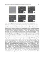
models employed and results obtained are illustrated in Figs.3-5. The sampling interval t0
is assumed to be equal to 0.1 s corresponding to Δz0= 15m. Models of a maximum-resolved
lidar profile Ps(z) and the corresponding detected lidar return Pl(z) [see Eq.(10)] in the case of
pulse response function f() given in the inset are shown in Fig.3. As can be seen, Ps(z)
consists of some mean profile, a high-resolution component in the near field, and a doublepeak structure introducing discontinuities at a further range. The system response function
f() is chosen to have a shape close to this of the typical TEA-CO2 laser pulses. It consists of
an initial spike followed by a long tail. As a result of the effect of convolution, important
information about the small-scale variations of the backscattering within the long-resolution
cell (about 200-300 m) is lost in the registered long-pulse profile Pl(z). In the absence of noise
the deconvolution procedures ensure accurate retrieval of the short-pulse profile Ps(z). Then
the restored profiles Psc(z) do not differ visibly from the original model Ps(z). As it is shown
in Gurdev et al., 1993, the systematic errors due to discrete data processing can be of the
order of or smaller than 1% on the average. The random noise influence on the retrieval
accuracy is simulated assuming that c1,2<<f,q,q<<f and even q<t0 as it is in the
atmospheric lidars. In this case, at comparable noise levels N1 and N2 , the influence of the
stationary background component N2 will be dominating [see Eqs.(11), (17), (24a), (29a), (33),
and (38)]. Therefore, we have simulated a stationary effective additive noise n
corresponding to the convolution of N2 and the receiving system response q. The correlation
time c of the noise n is of the order of q and may be both larger and smaller than Δt0. In the
latter case we have in practice a white noise with restricted frequency band (</Δt0) due to
sampling. The effective correlation time of such a noise is equal to Δt0. In the simulations we
have generated white noise (c~Δt0) and Gaussian-correlation noise (c>Δt0). The noise level
is specified by the (signal-to-noise, SNR) ratio of the minimum of the double-peak structure
of Ps(z) (see Fig.3) to the standard deviation of the noise n.
In Fig.4, the original short-pulse profile Ps(z) is compared with the profiles Psr(z) restored by

using Fourier deconvolution in the presence of white noise with SNR=50. As seen in Fig.4a, the
deconvolution leads to an increase of the noise influence and the error magnitude considerably
exceeds the oscillation amplitude of the retrieved profile. So, some type of controllable lowpass filtering is necessary, retaining at the same time an improved retrieval resolution. In


261

Deconvolution of Long-Pulse Lidar Profiles

Fig.4b such a filtering is realized by increasing the computing step up to t=4t0. The results
from filtering the measured lidar profiles Plm(z) by a smooth monotonic low-pass filter with
4t0-wide window are shown in Fig.4c. As seen, both types of processing lead to similar
restored profiles with considerable reduction of the noise effect [see Eq.(19)].
0.4

0.5

0.3

Laser Power

Power (arb. units)

0.6
0.4

0.2
0.1

0.3

0.0

0.2

0

2

4
6
8
Time ( s)

10

12

0.1
0.0

0

2

4

6 8 10 12 14
Range (km)

Fig. 3. Short-pulse lidar profile Ps(z) (red) and the corresponding detected lidar return Pl(z)
(blue) obtained for the pulse response shape f() (inset).

Power (arb. units)

(a)

0.5
0.0
-0.5

0

2

4

6 8 10 12 14
Range (km)

Power (arb. units)

Power (arb. units)

1.0

0.6
0.5
0.4
0.3

0.2
0.1
0.0

0.6
0.5
0.4
0.3
0.2
0.1
0.0

(b)

0

2

4

6 8 10 12 14
Range (km)

(c)

0

2

4

6 8 10 12 14
Range (km)

Fig. 4. Profile Ps(z) (red) and the profile restored by use of Fourier deconvolution (blue), in
the presence of white Gaussian-distributed noise with SNR=50, at t=t0 (a), t=4t0 (b),
and when using a smooth monotonic filter with a 4t0-wide window applied to the
measured lidar profile (c).


Lasers – Applications in Science and Industry

(a)

0.6
0.5
0.4
0.3
0.2
0.1
0.0
-0.1
0

2

4

6 8 10 12 14
Range (km)

(b)

0.6
Power (arb. units)

Power (arb. units)

262

0.4
0.2
0.0

0

2

4

6 8 10 12 14
Range (km)

Fig. 5. Profile Ps(z) (red) and the profile restored by use of Fourier deconvolution (blue) in
the presence of additive Gaussian correlated and distributed noise with SNR=50 and
correlation time c=2t0 (a) and 5t0 (b).
The effect of the correlated noise with c>t0 (i.e., c~q>t0) is gradually lower than that of
the white noise [see Eq.(19)]. It is illustrated in Fig.5 where the profiles Psr(z) are shown
restored by Fourier deconvolution in the presence of correlated Gaussian noise with c=2t0
and 5t0 and SNR=50. As expected, the error magnitude decreases with increasing the

correlation time of the noise and at c=5t0 the accuracy of the deconvolved lidar profiles is
satisfactory even without any filtering applied.
The efficiency of the Fourier deconvolution approach is demonstrated as well in Stoyanov et al.,
1996, where data (backscattering power profiles) have been processed, obtained by the National
Oceanic and Atmospheric Administration (NOAA) pulsed coherent CO2 Doppler lidar.
In Fig.6, the profile Pl(z) is shown obtained by convolution of Ps(z) with a rectangular-like
sensing laser pulse with =2 s and r =0.1 s. The recovered by algorithm (31) profiles Psr(z)
in the presence of white noise at SNR=50 are represented in Fig.7. As it is seen, the noise
influence is strong if no filtering is employed (Fig.7a). At the same time, increasing the
computing step [Eq.(34)] up to t=4t0 (Fig.7b) or filtering Plm(z) using a smooth monotonic
low-pass filter with 4t0-wide window (Fig.7c) lead to comparable substantial reduction of
the noise effect at minimum distortion of Psr(z) with respect to Ps(z). The intrinsic noise
0.5
0.4

0.5

Laser Powe r

Power (arb. units)

0.6

0.3

0.4

0.2
0.1

0.3

0.0

0

1
2
Time (s)

3

0.2
0.1
0.0

0

2

4

6 8 10 12 14
Range (km)

Fig. 6. Short-pulse lidar profile Ps(z) (red) and the corresponding detected lidar return Pl(z)
(blue) obtained for the rectangular-like pulse response shape f() given in the inset.


263

Deconvolution of Long-Pulse Lidar Profiles

accumulation with the range is also noticeable. In Fig.8 it is shown that the effect of a
correlated noise (with c~q>t0) on the retrieval accuracy is considerably lower compared to
the effect of white noise. In agreement with the theoretical results [Eq.(33)], the retrieval
error decreases with increasing the correlation time of the noise. At c=5t0 the accuracy of
the restored profiles is quite acceptable without any filtering performed.

(a)
Power (arb. units)

0.4
0.2
0.0
-0.2
-0.4

0

2

4

6 8 10 12 14
Range (km)
Power (arb. units)

Power (arb. units)

0.6

0.6
0.5
0.4
0.3
0.2
0.1
0.0

0.6
0.5
0.4
0.3
0.2
0.1
0.0

(b)

0

2

4

6 8 10 12 14
Range (km)

(c)

0

2

4

6 8 10 12 14
Range (km)

Fig. 7. Profile Ps(z) (red) and the profile restored by use of Fourier deconvolution (blue), in
the presence of white Gaussian-distributed noise with SNR=50, at t=t0 (a), t=4t0 (b),
and when using a smooth monotonic filter with a 4t0-wide window applied to the
measured lidar profile (c).
The investigations described in this section show that deconvolution techniques can be
successfully used for improving the accuracy and resolution of sensing the atmosphere or
other objects by long-pulse elastic direct-detection lidars. At negligibly weak noise a high
accuracy in the restoration of the short-pulse lidar profile is achievable at short-enough
computing step. Also, the uncertainties in the lidar pulse response function lead to some
characteristic retrieval distortions that can be reduced to some extent by using suitable
approaches. Even at high initial SNR, a broadband noise, i.e., fast fluctuations with
correlation time below the sensing-pulse duration, can cause considerable noise effect such
that the retrieved short-pulse lidar profile is fully disguised. In this case, the noise influence
can be effectively reduced by using appropriate filtering or choice of the computing step.
The filter window or the computing step should exceed the fluctuation correlation time. At


264

Lasers – Applications in Science and Industry

0.6

(a)

Power (arb. units)

Power (arb. units)

0.6
0.4
0.2
0.0
0

2

4

6 8 10 12 14
Range (km)

(b)

0.4
0.2
0.0
0

2

4

6 8 10 12 14
Range (km)

Fig. 8. Profile Ps(z) (red) and the profile restored by use of Fourier deconvolution (blue) in
the presence of additive Gaussian correlated and distributed noise with SNR=50 and
correlation time c=2t0 (a) and 5t0 (b).
the same time, they should be smaller than the least variation scale of the short-pulse lidar
profile to avoid essential distortions and lowering of the retrieval resolution. Note as well
that the deconvolution algorithm performance decreases the effect of narrow-band noise
whose correlation time substantially exceeds the pulse duration. At last, let us mention one
more virtue of the deconvolution-based retrieval of the short-pulse lidar profiles. That is, it
allows high-resolution sensing of small finite-size objects by longer laser pulses, realizing in
this way double-sided linear-strategy optical tomography of such objects.

4. Deconvolution-based improvement of the accuracy of measuring electron
temperature profiles in tokamak plasmas by Thomson scattering lidar
The electron temperature Te and density ne distributions in the torus are basic characteristics of
the tokamak fusion plasma. They are conditioned by the modes of heating and confinement of
the high-temperature plasma as well as by the different oscillatory movements of the plasma
particles sometimes leading to the appearance of crucial instabilities. Thus, the Te and ne
profiles are not only important factors of the development and the efficiency of the fusion
process but indicators as well of the dynamic plasma state. So far, the most appropriate
approach to their simultaneous express determination in a remote contactless way is the
Thomson scattering (TS) lidar approach (Salzmann et al., 1988; Kempenaars et al., 2008, 2010).
It allows one to obtain the Te and ne profiles along a LOS through the torus core. The minimum
range resolution interval achievable by the contemporary core TS lidars (Kempenaars et al.,
2010) is about 12-15 cm. Such a resolution is relatively good in general, but is insufficient for

resolving small-scale inhomogeneities and the edge pedestal areas of Te and ne profiles in the
so-called high-confinement mode (H-mode) of operation of the tokamak reactors. A way of
improving the range resolution of the TS lidars is based on the use of deconvolution
techniques for recovering the high-resolution lidar profiles. The deconvolution procedures,
however, increase the influence of the noise. Therefore, to achieve acceptable recovered
profiles one should apply a final filtering that lowers the sensing resolution to some
compromise extent. The statistical modeling is a way to outline some optimal conditions under
which the deconvolution techniques lead to satisfactory high-resolution restoration of the Te
profiles (Stoyanov et al., 2009; Dreischuh et al., 2011).


265

Deconvolution of Long-Pulse Lidar Profiles

The TS lidar return signal from fussion plasma as well as the plasma light background and
other additive noise are convenient to be analyzed on the basis of an equivalent photon
counting procedure (Gurdev et al., 2008b). Based on Eqs.(1), (4) and (9), the long-pulse lidar
equation in this case, for some say m-th spectral interval [s1m,s2m], is expressible as
z

N l ( s 1m , s 2 m ; z)  N lm ( z)   2 / c   dz ' f [2( z  z ') / c ]N s (s 1m , s 2 m ; z) ,
0

(46)

where the maximum-resolved lidar profile Ns is described by the short-pulse lidar equation
N s (s 1m , s 2 m ; z )  N sm ( z )  (c / 2) AN 0 (i )

s 2 m

s 1 m

dsK (i , s )(i , s ; z ) ;

(47)

K(i,s)=Kt(i)Kt(s)Kf(s)EQE(s); Kt(i), Kt(s), Kf(s) and EQE(s) are respectively the
wavelength-dependent optical transmittance of the plasma-irradiating path, the optical
transmittance of the scattered-light collecting path, the receiver filter spectral characteristic,
and the effective quantum efficiency of the photon detection accounting for the quantum
yield and the Poisson fluctuations of the photoelectron number after the photocathode
enhanced in the process of cascade multiplying in the employed microchannel tube;
(i,s;z) is given by Eq.(2) with T(i,s;z) 1, (i;z)=(z)=ne(z)r02, and
1

L[s , i ; z] 


2
4

c
15 vth ( z) 105 vth ( z)  (i / s )3

1 

2
16 c
512 c 4  (1  i / s )

 i vth ( z) 



 c2


(i / s )1/2  (s / i )1/2  2   q[ i , s , Te ( z)]
exp  2


 vth ( z)




;

(48)

r0=e2/(40mec2) is the classical electron radius, e and me are respectively the electron charge
and rest mass, 0 is the dielectric constant of vacuum, vth(z)=[2kBTe(z)/me]1/2 is the rms
thermal velocity of the electrons, kB is the Boltzmann constant, ne(z) and Te(z) are
respectively the electron density and temperature profiles along the lidar LOS, and
q[i,s,Te(z)] is the depolarization term accounting for the relativistic depolarization effects
on the backscattered radiation. For scattering at 180o the depolarization can be expressed in
terms of exponential integral En(p) (Naito et al., 1993):

q[i , s , Te ( z)]  1  2 e p  E3 ( p )  3E5 ( p )  1 

p

me c 2
2 kBTe ( z)







p2 
1  p3 p2


 p  1  p 2  1   e p E1 ( p )
 


2 2
2
4 





(49)

  px

e
dx .
n
1 x

s / i  i / s , and En ( p )  

The TS lidar signal is accompanied by the plasma light background that is a serious source
of error in the determination of Te. Its emissivity spectrum per unit solid angle, mainly due
to the bremsstrahlung, is given by the expression (Sheffield, 1975; Foord et al., 1982) :


dE 0.95  10 19 2
hc


ne ( z)Zeff ( z)[ kBTe ( z)]1/2 exp  
 g ff ( , Te ) ,
d
 4
 kBTe ( z) 


(50)


266

Lasers – Applications in Science and Industry

where Zeff (z) is the effective ion charge, the quantities kBTe and hc/ are in eV, exp[-hc/

(kBTe)]1 and g ff ( , Te ) is the so-called Gaunt factor that depends weakly on Te and on the
radiation wavelength , and accounts for the quantum effects, the electron screening of
nuclei, etc. (Brusaard & van de Hulst, 1962). For the photoelectron rate characterizing the
parasitic background due to plasma light penetrating into the m-th spectral channel we
obtain the following expression:

N bm (s1m , s2 m )  6.25  1021 ADD
2
 dzne ( z) kBTe ( z)

1/2

z

s 2 m



s 1 m

dsKt (s )K f (s )EQE(s )s1 ln  kBTe ( z) /(13.6h 2c 2 / s2 )1/3  ,



(51)

where AD is the photon detector effective area and D is the solid angle determined by the

relative aperture of the receiving optics. In order to take into account additional background
light sources, an enhancement factor is included in the simulations.
The center-of-mass wavelength (CMW) approach (Gurdev et al., 2008b; Dreischuh et al.,
2009) to the determination of the electron temperature profiles Te(z) in fusion plasma is
based on the unambiguous temperature dependence of the CMW of the relativistic
Thomson backscattering spectrum. The TS lidar profiles Nsm are measured for M selected
spectral intervals [s1m,s2m] (m=1,2,…,M) [see Eq.(48)]. The CMW CM defined as


 



CM (Te ; z)    m N sm ( z)  /   N sm ( z) 


 

m

m

(52)



is unambiguous function of the electron temperature (see also Fig.10 below);

m=(s1m+s2m)/2 is the central wavelength of the m-th interval. Then the temperature is
determined on the basis of the inverse function Te(CM,z).

The linear error propagation approach leads to the following expression of the rms error Te
in the determination of Te on the basis of the dependence CM= f(Te) (Gurdev et al., 2008b):
 Te  d ln CM (Te ) / dTe

1 


  N pm q 
m


1  M

1/2

2

  m  CM 

 N pm q (1  N bm / N pm )
 
CM 
m1 





, (53)

where Npm is the convolution of the laser pulse shape and the short-pulse lidar profile. The
determinant temporal factor in Eq.(53) is q because it is in practice the signal integration
time interval. In case of applying deconvolution techniques for recovering the short-pulse
lidar profiles and thus for obtaining more accurate Te profiles, instead of Eq.(53) we have
(Dreischuh et al., 2011)

 Te  d ln CM (Te ) / dTe

1 


  Nsm 
m


1  M

1/2

2

  m  CM 

 Nsm [1   ( s / )Nbm / Nsm ]

CM 
m1 


,

(54)

where  is the time-domain filter window and the factor (s/) is an increasing function
of the ratio s/. This factor is accounting for the fact that the background is initially


Deconvolution of Long-Pulse Lidar Profiles

267

smoothed (integrated) only by the receiving system response function while the
deconvolution is performed using the total lidar response function including the laser
pulse shape.
An estimate of the SNR for the m-th spectral channel could be written as follows:
SNRm  { N pm q /(1  N bm / N pm )} 1/2

(55)

in the case of convolved lidar profiles, and
SNRm  { N sm  /(1   ( s /  )N bm / N sm )} 1/2

(56)

in the case of deconvolved lidar profiles.
From Eqs.(53-56) evidently follows that the signal-to-noise ratios SNRm are the main factor
conditioning the statistical retrieval accuracy.
The characteristic parameters of the plasma and the TS lidar used in the simulations are
chosen to be close to those of the core TS lidar system on the Joint European Torus (JET)
(Casci et al., 2002; Salzmann et al., 1988; Kempenaars et al., 2008, 2010). The sensing laser

radiation is assumed to have wavelength i=694 nm and pulse energy E0=N0hc/i=1 J, and
to be injected horizontally along the plasma midplane. The minor radius r of the torus, along
the LOS, is supposed to be 1 m. Correspondingly, the plasma is supposed to occupy the
region between R=2 m and R=4 m, R being the radial distance from the center of the torus
(Casci et al., 2002). Assuming that the LOS coordinate of the center of the torus is zc, we
obtain that R=zc- z. The number of receiving spectrometer channels is chosen to be six. Their
absolute spectral responses, including the EQE of the detectors, are also close to those of JET
TS core lidar (Kempenaars et al., 2010). In particular, the detectors considered in the
simulations are multialkali microchannel plate photomultiplier tubes (MCP-PMTs) with
response times of about 650 ps and EQE equal to 0.005 for channel 1 and 0.02 for the other
five channels. TS spectrum is observed within the wavelength region from 350 nm to 850
nm. To correct the collection efficiency the values of the solid angle of acceptance given in
Kempenaars et al., 2010 are used. They vary from 0.005 sr, at R=2 m, to 0.007 sr at R=4 m.
The irradiating and collecting paths optical transmittances assumed are Kt(i)=0.75 and
Kt(s)=0.25, respectively. The detector’s etendue E=ADD needed for the estimation of the
plasma bremsstrahlung photoelectron rate is assumed to have a value of ~0.32 cm2sr. The
factor of reducing the plasma bremsstrahlung conditioned by the plasma torus observation
pupil is supposed to be 0.3. The effective atomic number of an equivalent plasma ion is
chosen to be Zeff=2. The bremsstrahlung background is added multiplied by an
enhancement factor of 2 in order to take into account additional background light sources.
The temporal sampling interval t0 is supposed to be 200 ps (z0=3 cm spatial interval).
The models of the temperature and density profiles used in the simulations consist of a
smooth parabolic component whose parameters are chosen to simulate the real plasma
conditions (Dreischuh et al., 2011; see also Figs. 12-14). Additionally, the Te(z) profile has a
multiscale high-resolution component superimposed on the smooth component in order to
illustrate the improvement of the retrieval accuracy and resolution depending on the noise
level. The central electron density is varied in the range ne= 2  9 x1019 m-3 to simulate
different plasma conditions and SNRs.
The sensing laser pulse shape is chosen to be s() = (/l2) exp(-/l) for  0 and s() = 0 for
< 0, where l is a time constant. Such a pulse shape can be a good approximation of various

268

Lasers – Applications in Science and Industry
9

Pulse shape [arb. units]

3.0x10

Laser
Receiving electronics
TS Lidar

9

2.5x10

9

2.0x10

9

1.5x10

9

1.0x10

8

5.0x10

0.0
0.0

-10

-9

-9

-9

5.0x10 1.0x10 1.5x10 2.0x10
Time [s]

Center-of-mass wavelength [nm]

Fig. 9. Models of the laser pulse shape (circles), receiving system response shape (triangles)
and the resulting TS lidar system response shape (stars) used in the simulations.

750
700
650
600
550

0

1

2 3 4 5 6 7 8 9 10
Electron temperature [keV]

Fig. 10. Reference function CM(Te) underlying the CMW approach.
real asymmetric laser pulses (e.g., Dong et al., 2001; Kondoh et al., 2001). The same model is
used for the shape of the receiving system response function q(), that is, q() = (/e2)exp(/e) for 0, and q() = 0 for <0, where e is another time constant. The Fourier spectrum
modulus of the above pulse shapes is equal to (1+2l,e2)-1, i.e., it has no zeros, which is
favorable for applying Fourier-deconvolution algorithm. The values of l and e are chosen
so that the effective durations s=el and q=ee of s() and q() to be respectively about 350 ps
(l = 130 ps) and 810 ps (e= 300 ps). Then the effective duration of the resulting system
response shape f will be about 1 ns, which corresponds to 15 cm range resolution cell of the
TS lidar. The models of the laser pulse shape, the receiving system response shape and the
TS lidar system response shape are shown in Fig.9.
The reference function CM(Te) is determined on the basis of the temperature dependence of
the TS spectrum and is presented in Fig.10 for temperatures up to 10 keV. In the case of
long-pulse sensing, when the pulse length exceeds the spatial scale of the temperature
inhomogeneities, the temperature information provided by the lidar profiles from the
different spectral channels will be distorted. Correspondingly, the recovered temperature


269

Deconvolution of Long-Pulse Lidar Profiles

profiles will also be distorted with respect to the true ones. The role of the deconvolution
here is to reduce, as much as possible at the corresponding noise level, the convolution-due

distortions of the recovered Te profiles.
The Monte-Carlo simulations are performed in the following way. First, the mean values
Nsm(z) of the TS signal in each spectral channel are determined and then convolved with the
laser pulse shape in order to account for the real pulse duration. Next, the mean background
photoelectron count rate Nbm(z) is evaluated. Then, assuming Poisson statistics of the signal
and background photoelectrons within a t0 - long interval and using random –
number generator, J realizations of the TS signal Nlm(z)t0 and background Nbm(z)t0
photoelectrons are produced (see Fig11). Further, the receiving system response function is
taken into account performing the convolution with it of the profiles of the background and
signal count rates in each channel. Assuming an accurate measurement of the mean
convolved background count rate, it is subtracted from the corresponding background
count rate realizations. Thus, the convolved background count rate fluctuations are
obtained. At last, the obtained realizations of the long-pulse lidar profiles including the
background fluctuations are deconvolved using the system response function f(). The
center of mass wavelength as a function of the coordinate along the LOS is determined
according to Eq.(52) on the basis of the deconvolved profiles, and is used together with the
ˆ
reference function CM(Te) for obtaining J estimates T ( z) of the electron temperature
ej

ˆ
profile Te(z), j=1,2,…,J. Then, an estimate  Te ( z) of the measurement error is obtainable as

Number of photoelectrons

350
300
250
200

J



1/2

.

(a)

1st channel
2nd channel
3rd channel
4th channel
5th channel
6th channel

150
100
50
0
2.0

2.5

3.0
Radius [m]

3.5

4.0

350
Number of photoelectrons



ˆ
ˆ
 Te ( z)  J 1  j  1[Tej ( z)  Te ( z)]2

300
250
200

(b)

1st channel
2nd channel
3rd channel
4th channel
5th channel
6th channel

150
100
50
0
2.0

2.5

3.0
Radius [m]

3.5

4.0

Fig. 11. TS lidar profiles: (a) mean short-pulse lidar profiles including the mean plasma light
background, (b) realizations of the measured long-pulse lidar profiles including the
background realizations; ne = 9x1019 m-3 .
To simulate correctly the detection of the analog signals, the convolved profiles are
calculated almost ideally by a computing step much less than t0. The real ADC step t0 is
used when processing further the long-pulse profiles. The obtained mean short-pulse lidar
profiles and simulated realizations of the measured long-pulse lidar profiles for the six
spectral channels are shown in Figs.11a,b.


270

Lasers – Applications in Science and Industry

Аs an illustration of the deconvolution effect, the Te profiles restored in the absence of noise
on the basis of the convolved and deconvolved lidar profiles are shown in Fig.12. As it is
seen, the direct use of the long-pulse lidar profiles leads to significant distortions in the
restored electron temperature profiles. After applying deconvolution techniques to the longpulse lidar profiles, at negligible noise level the Te profiles are determined with considerably
higher accuracy, and resolution scale of the order of the sampling interval z0.
Because of the strong Poisson fluctuations, some type of low-pass noise filtering is necessary
to ensure a satisfactory quality of the restored profiles. However, the filtering procedure

lowers the range resolution. The range resolution cell will be already of the order of the
width W of the range-domain window of the filter employed. To retain a satisfactory range
resolution the value of W should be less than the least variation scale (along the line of sight)
of the temperature profile. Then the restored temperature profiles are minimally distorted
with respect to the true ones. Different low-pass digital filters are used in the numerical
simulations. Results presented below are obtained using filers with 2z0 and 3z0 –wide
windows for smoothing the recorded lidar profiles.

Model
Restored

(a)

5
4
3
2
1
0

2.0

2.5
3.0
Radius [m]

3.5

4.0

6
Electron temperature [keV]

Electron temperature [keV]

6

Model
Restored

(b)

5
4
3
2
1
0
2.0

2.5

3.0
Radius [m]

3.5

4.0

Fig. 12. Electron temperature profiles restored in absence of noise on the basis of the

convolved (a) and deconvolved (b) lidar profiles; ne = 9x1019 m-3.
In Fig.13 the profiles of the electron temperature restored on the basis of the measured
convolved and deconvolved lidar profiles for one realization of the Poisson noise are
presented. It is well seen that the temperature profiles restored on the basis of convolved
lidar profiles (Fig.13a) are essentially distorted with respect to the original model. At the
same time, the temperature profile restored on the basis of deconvolved lidar profiles
(Fig.13b) is disguised by strongly increased fluctuations. In order to suppress the
deconvolution-due increase of the noise, noise controlling filters have been applied
(Figs.13c,d) ensuring acceptable accuracy and resolution of the restored electron
temperature profiles. It is seen in Fig.13d that even 2z0–wide filter window (corresponding
to 6 cm range resolution) ensures good quality of the obtained Te profile. The theoretical
statistical errors presented in these figures are estimated assuming empirically in Eq.(54)
that (s/) = 25 (Fig.13b), 15 (Fig.13c), and 10 (Fig.13d). When using convolved profiles
for determination of Te (Fig.13a), the factor (s/) is not of importance [Eq.(53)]. In this