RECENT ADVANCES IN ROBUST CONTROL – NOVEL APPROACHES AND DESIGN METHODSE Part 5 pdf

Neural Control Toward a Unified
Intelligent Control Design Framework for Nonlinear Systems

109
Define
12
() () ()xt x t x tΔ= − , and
ˆ
p
pp
Δ
=−. Then we have
0
0
1
() { () ()()] ()}
(())
t
TT T
t
t
t
xt a xs B xsus C xspds
C x s pds
Δ
=Δ+Δ +Δ +
Δ
∫
∫

If the both sides of the above equation takes an appropriate norm and the triangle inequality

is applied, the following is obtained:
0
0
1
|| ( )|||| { ( ) ( ) ( )] ( ) } ||
|| ( ( )) ||
t
TT T
t
t
t
xt a xs B xsus C xspds
Cx s p ds
Δ
≤Δ+Δ +Δ +
Δ
∫
∫

Note that
1
|| ( ( ) ||Cx s p
Δ
can be made uniformly bounded by
ε
as long as the estimate of
p
is made sufficiently close to
p
(which can be controlled by the granularity of tessellation),

and
p
is bounded; |()|1ut
≤
; || || sup ( )
TxT
aax
∈Ω
=
<∞, || || sup ( )
TxT
BBx
∈Ω
=
<∞and
|| || sup ( )
TxT
CCx
∈Ω
=<∞
.
It follows that
0
0
|| ( )|| ( ) (|| || || || || |||| ||) ( )
t
TTT
t
xt t t a B C p xsds
ε

Δ≤−+ + + Δ
∫

Define a constant
0
(|| || || || || |||| ||)
TTT
Ka B Cp=++
. Applying the Gronwall-Bellman
Inequality to the above inequality yields
0
000 0
2
0
00 00
|| ( )|| ( ) ( )exp{ }
()
() exp(())
2
tt
ts
xt t t K s t Kd ds
tt
tt K Ktt K
εε σ
εε ε
Δ≤−+ −
−
≤−+ − ≤
∫∫

where
0
00 00
()
( )(1 exp( ( )))
2
tt
Ktt K Ktt
−
=− + −
, and K
<
∞ .
This completes the proof.
6. Simulation
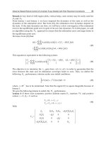
Consider the single-machine infinity-bus (SMIB) model with a thyristor-controlled series-
capacitor (TCSC) installed on the transmission line (Chen, 1998) as shown in Fig. 5, which
may be mathematically described as follows:

0
(1)
1
((1) sin)
(1 )
b
t
m
de
VV

PPD
MXsX
ωω
δ
ω
δ
ω
−
⎡
⎤
⎡⎤
⎢
⎥
=
∞
⎢⎥
⎢
⎥
−− −−
⎣⎦
⎢
⎥
+−
⎣
⎦




Recent Advances in Robust Control – Novel Approaches and Design Methods

110
where
δ
is rotor angle (rad),
ω
rotor speed (p.u.), 260
b
ω
π
=
× synchronous speed as base
(rad/sec),
0.3665
m
P =
is mechanical power input (p.u.),
0
P
is unknown fixed load (p.u.),
2.0D = damping factor, 3.5M
=
system inertia referenced to the base power, 1.0
t
V =
terminal bus voltage (p.u.),
0.99V
∞
=
infinite bus voltage (p.u.), 2.0

d
X
=
transient
reactance of the generator (p.u.),
0.35
e
X = transmission reactance (p.u.),
min max
[ , ] [0.2,0.75]ss s∈= series compensation degree of the TCSC, and (,1)
e
δ
is system
equilibrium with the series compensation degree fixed at
0.4
e
s = .
The goal is to stabilize the system in the near optimal time control fashion with an
unknown load
0
P ranging 0 and 10% of
m
P . Two nominal cases are identified. The
nominal neural networks have 15 and 30 neurons in the first and second hidden layer
with log-sigmoid and tan-sigmoid activation functions for these two hidden layers,
respectively. The input data to regional neural networks is the rotor angle, its two
previous values, the control and its previous value, and the outputs are the weighting
factors. The regional neural networks have 15 and 30 neurons in the first and second
hidden layer with log-sigmoid and tan-sigmoid activation functions for these two hidden
layers, respectively. The global neural networks are really not necessary in this simple

case of parameter uncertainty.
Once the nominal and regional neural networks are trained, they are used to control the
system after a severe short-circuit fault and with an unknown load (5% of
m
P ). The resulting
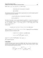
trajectory is shown in Fig. 6. It is observed that the hierarchical neural controller stabilizes
the system in a near optimal control manner.













Fig. 5. The SMIB system with TCSC
Synchronous
Machine
Transmission
Line with TCSC
Infinite
Bus
Neural Control Toward a Unified
Intelligent Control Design Framework for Nonlinear Systems

111


Fig. 6. Control performance of hierarchical neural controller. Solid - neural control; dashed -
optimal control.
7. Conclusion
Even with remarkable progress witnessed in the adaptive control techniques for the
nonlinear system control over the past decade, the general challenge with adaptive control
of nonlinear systems has never become less formidable, not to mention the adaptive control
of nonlinear systems while optimizing a pre-designated control performance index and
respecting restrictions on control signals. Neural networks have been introduced to tackle
the adaptive control of nonlinear systems, where there are system uncertainties in
parameters, unmodeled nonlinear system dynamics, and in many cases the parameters may
be time varying. It is the main focus of this Chapter to establish a framework in which
general nonlinear systems will be targeted and near optimal, adaptive control of uncertain,
time-varying, nonlinear systems is studied. The study begins with a generic presentation of
the solution scheme for fixed-parameter nonlinear systems. The optimal control solution is
presented for the purpose of minimum time control and minimum fuel control, respectively.
The parameter space is tessellated into a set of convex sub-regions. The set of parameter
vectors corresponding to the vertexes of those convex sub-regions are obtained.
Accordingly, a set of optimal control problems are solved. The resulting control trajectories
and state or output trajectories are employed to train a set of properly designed neural
networks to establish a relationship that would otherwise be unavailable for the sake of near
optimal controller design. In addition, techniques are developed and applied to deal with
the time varying property of uncertain parameters of the nonlinear systems. All these pieces

Recent Advances in Robust Control – Novel Approaches and Design Methods

112
come together in an organized and cooperative manner under the unified intelligent control

design framework to meet the Chapter’s ultimate goal of constructing intelligent controllers
for uncertain, nonlinear systems.
8. Acknowledgment
The authors are grateful to the Editor and the anonymous reviewers for their constructive
comments.
9. References
Chen, D. (1998). Nonlinear Neural Control with Power Systems Applications, Doctoral
Dissertation, Oregon State University, ISBN 0-599-12704-X.
Chen, D. & Mohler, R. (1997). Load Modelling and Voltage Stability Analysis by Neural
Network, Proceedings of 1997 American Control Conference, pp. 1086-1090, ISBN 0-
7803-3832-4, Albuquerque, New Mexico, USA, June 4-6, 1997.
Chen, D. & Mohler, R. (2000). Theoretical Aspects on Synthesis of Hierarchical Neural
Controllers for Power Systems, Proceedings of 2000 American Control Conference, pp.
3432 – 3436, ISBN 0-7803-5519-9, Chicago, Illinois, June 28-30, 2000.
Chen, D. & Mohler, R. (2003). Neural-Network-based Loading Modeling and Its Use in
Voltage Stability Analysis. IEEE Transactions on Control Systems Technology, Vol. 11,
No. 4, pp. 460-470, ISSN 1063-6536.
Chen, D., Mohler, R., & Chen, L. (1999). Neural-Network-based Adaptive Control with
Application to Power Systems, Proceedings of 1999 American Control Conference, pp.
3236-3240, ISBN 0-7803-4990-3, San Diego, California, USA, June 2-4, 1999.
Chen, D., Mohler, R., & Chen, L. (2000). Synthesis of Neural Controller Applied to Power
Systems. IEEE Transactions on Circuits and Systems I, Vol. 47, No. 3, pp. 376 – 388,
ISSN 1057-7122.
Chen, D. & Yang, J. (2005). Robust Adaptive Neural Control Applied to a Class of Nonlinear
Systems, Proceedings of 17th IMACS World Congress: Scientific Computation, Applied
Mathematics and Simulation, Paper T5-I-01-0911, pp. 1-8, ISBN 2-915913-02-1, Paris,
July 2005.
Chen, D., Yang, J., & Mohler, R. (2006). Hierarchical Neural Networks toward a Unified
Modelling Framework for Load Dynamics. International Journal of Computational
Intelligence Research, Vol. 2, No. 1, pp. 17-25, ISSN 0974-1259.

Chen, D., Yang, J., & Mohler, R. (2008). On near Optimal Neural Control of Multiple-Input
Nonlinear Systems. Neural Computing & Applications, Vol. 17, No. 4, pp. 327-337,
ISSN 0941-0643.
Chen, D., Yang, J., & Mohler, R. (2006). Hierarchical Neural Networks toward a Unified
Modelling Framework for Load Dynamics. International Journal of Computational
Intelligence Research, Vol. 2, No. 1, pp. 17-25, ISSN 0974-1259.
Chen, D. & York, M. (2008). Neural Network based Approaches to Very Short Term Load
Prediction, Proceedings of 2008 IEEE Power and Energy Society General Meeting, pp. 1-
8, ISBN 978-1-4244-1905-0, Pittsbufgh, PA, USA, July 20-24, 2008.
Neural Control Toward a Unified
Intelligent Control Design Framework for Nonlinear Systems

113
Chen, F. & Liu, C. (1994). Adaptively Controlling Nonlinear Continuous-Time Systems
Using Multilayer Neural Networks. IEEE Transactions on Automatic Control, Vol. 39,
pp. 1306–1310, ISSN 0018-9286.
Haykin, S. (2001). Neural Networks: A Comprehensive Foundation, Prentice-Hall, ISBN
0132733501, Englewood Cliffs, New Jersey.
Hebb, D. (1949). The Organization of Behavior, John Wiley and Sons, ISBN 9780805843002,
New York.
Hopfield, J. J., & Tank, D. W. (1985). Neural Computation of Decisions in Optimization
Problems. Biological Cybernetics, Vol. 52, No. 3, pp. 141-152.
Irwin, G. W., Warwick, K., & Hunt, K. J. (1995). Neural Network Applications in Control, The
Institution of Electrical Engineers, ISBN 0906048567, London.
Kawato, M., Uno, Y., & Suzuki, R. (1988). Hierarchical Neural Network Model for Voluntary
Movement with Application to Robotics. IEEE Control Systems Magazine, Vol. 8, No.
2, pp. 8-15.
Lee, E. & Markus, L. (1967). Foundations of Optimal Control Theory, Wiley, ISBN 0898748070,
New York.
Levin, A. U., & Narendra, K. S. (1993). Control of Nonlinear Dynamical Systems Using

Neural Networks: Controllability and Stabilization. IEEE Transactions on Neural
Networks, Vol. 4, No. 2, pp. 192-206.
Lewis, F., Yesidirek, A. & Liu, K. (1995). Neural Net Robot Controller with Guaranteed
Tracking Performance. IEEE Transactions on Neural Networks, Vol. 6, pp. 703-715,
ISSN 1063-6706.
Liang, R. H. (1999). A Neural-based Redispatch Approach to Dynamic Generation
Allocation. IEEE Transactions on Power Systems, Vol. 14, No. 4, pp. 1388-1393.
Methaprayoon, K., Lee, W., Rasmiddatta, S., Liao, J. R., & Ross, R. J. (2007). Multistage
Artificial Neural Network Short-Term Load Forecasting Engine with Front-End
Weather Forecast. IEEE Transactions Industry Applications, Vol. 43, No. 6, pp. 1410-
1416.
Mohler, R. (1991). Nonlinear Systems Volume I, Dynamics and Control, Prentice Hall,
Englewood Cliffs, ISBN 0-13-623489-5, New Jersey.
Mohler, R. (1991). Nonlinear Systems Volume II, Applications to Bilinear Control, Prentice Hall,
Englewood Cliffs, ISBN 0-13- 623521-2, New Jersey.
Mohler, R. (1973). Bilinear Control Processes, Academic Press, ISBN 0-12-504140-3, New York.
Moon S. (1969). Optimal Control of Bilinear Systems and Systems Linear in Control, Ph.D.
dissertation, The University of New Mexico.
Nagata, S., Sekiguchi, M., & Asakawa, K. (1990). Mobile Robot Control by a Structured
Hierarchical Neural Network. IEEE Control Systems Magazine, Vol. 10, No. 3, pp. 69-
76.
Pandit, M., Srivastava, L., & Sharma, J. (2003). Fast Voltage Contingency Selection Using
Fuzzy Parallel Self-Organizing Hierarchical Neural Network. IEEE Transactions on
Power Systems, Vol. 18, No. 2, pp. 657-664.
Polycarpou, M. (1996). Stable Adaptive Neural Control Scheme for Nonlinear Systems. IEEE
Transactions on Automatic Control, Vol. 41, pp. 447-451, ISSN 0018-9286.

Recent Advances in Robust Control – Novel Approaches and Design Methods

114

Sanner, R. & Slotine, J. (1992). Gaussian Networks for Direct Adaptive Control. IEEE
Transactions on Neural Networks, Vol. 3, pp. 837-863, ISSN 1045-9227.
Yesidirek, A. & Lewis, F. (1995). Feedback Linearization Using Neural Network. Automatica,
Vol. 31, pp. 1659-1664, ISSN.
Zakrzewski, R. R., Mohler, R. R., & Kolodziej, W. J. (1994). Hierarchical Intelligent Control
with Flexible AC Transmission System Application. IFAC Journal of Control
Engineering Practice, pp. 979-987.
Zhou, Y. T., Chellappa, R., Vaid, A., & Jenkins B. K. (1988). Image Restoration Using a
Neural Network. IEEE Transactions on Acoustics, Speech, and Signal Processing, Vol.
36, No. 7, pp. 1141-1151.
6
Robust Adaptive Wavelet Neural Network
Control of Buck Converters
Hamed Bouzari
*1,2
, Miloš Šramek
1,2
,
Gabriel Mistelbauer
2
and Ehsan Bouzari
3

1
Austrian Academy of Sciences
2
Vienna University of Technology
3
Zanjan University
1,2

Austria
3
Iran
1. Introduction
Robustness is of crucial importance in control system design because the real engineering
systems are vulnerable to external disturbance and measurement noise and there are always
differences between mathematical models used for design and the actual system. Typically, it
is required to design a controller that will stabilize a plant, if it is not stable originally, and to
satisfy certain performance levels in the presence of disturbance signals, noise interference,
unmodelled plant dynamics and plant-parameter variations. These design objectives are best
realized via the feedback control mechanism (Fig. 1), although it introduces in the issues of
high cost (the use of sensors), system complexity (implementation and safety) and more
concerns on stability (thus internal stability and stabilizing controllers) (Gu, Petkov, &
Konstantinov, 2005). In abstract, a control system is robust if it remains stable and achieves
certain performance criteria in the presence of possible uncertainties. The robust design is to
find a controller, for a given system, such that the closed-loop system is robust.
In this chapter, the basic concepts and representations of a robust adaptive wavelet neural
network control for the case study of buck converters will be discussed.
The remainder of the chapter is organized as follows: In section 2 the advantages of neural
network controllers over conventional ones will be discussed, considering the efficiency of
introduction of wavelet theory in identifying unknown dependencies. Section 3 presents an
overview of the buck converter models. In section 4, a detailed overview of WNN methods is
presented. Robust control is introduced in section 5 to increase the robustness against noise by
implementing the error minimization. Section 6 explains the stability analysis which is based
on adaptive bound estimation. The implementation procedure and results of AWNN
controller are explained in section 7. The results show the effectiveness of the proposed
method in comparison to other previous works. The final section concludes the chapter.
2. Overview of wavelet neural networks
The conventional Proportional Integral Derivative (PID) controllers have been widely used
in industry due to their simple control structure, ease of design, and inexpensive cost (Ang,

Recent Advances in Robust Control – Novel Approaches and Design Methods
116
Chong, & Li, 2005). However, successful applications of the PID controller require the
satisfactory tuning of parameters according to the dynamics of the process. In fact, most PID
controllers are tuned on-site. The lengthy calculations for an initial guess of PID parameters
can often be demanding if we know a few about the plant, especially when the system is
unknown.


Fig. 1. Feedback control system design.
There has been considerable interest in the past several years in exploring the applications of
Neural Network (NN) to deal with nonlinearities and uncertainties of the real-time control
system (Sarangapani, 2006). It has been proven that artificial NN can approximate a wide
range of nonlinear functions to any desired degree of accuracy under certain conditions
(Sarangapani, 2006). It is generally understood that the selection of the NN training
algorithm plays an important role for most NN applications. In the conventional gradient-
descent-type weight adaptation, the sensitivity of the controlled system is required in the
online training process. However, it is difficult to acquire sensitivity information for
unknown or highly nonlinear dynamics. In addition, the local minimum of the performance
index remains to be challenged (Sarangapani, 2006). In practical control applications, it is
desirable to have a systematic method of ensuring the stability, robustness, and performance
properties of the overall system. Several NN control approaches have been proposed based
on Lyapunov stability theorem (Lim et al., 2009; Ziqian, Shih, & Qunjing, 2009). One main
advantage of these control schemes is that the adaptive laws were derived based on the
Lyapunov synthesis method and therefore it guarantees the stability of the under control
system. However, some constraint conditions should be assumed in the control process, e.g.,
that the approximation error, optimal parameter vectors or higher order terms in a Taylor
series expansion of the nonlinear control law, are bounded. Besides, the prior knowledge of
the controlled system may be required, e.g., the external disturbance is bounded or all states

of the controlled system are measurable. These requirements are not easy to satisfy in
practical control applications.
NNs in general can identify patterns according to their relationship, responding to related
patterns with a similar output. They are trained to classify certain patterns into groups, and
then are used to identify the new ones, which were never presented before. NNs can
correctly identify incomplete or similar patterns; it utilizes only absolute values of input
variables but these can differ enormously, while their relations may be the same. Likewise
we can reason identification of unknown dependencies of the input data, which NN should
learn. This could be regarded as a pattern abstraction, similar to the brain functionality,
where the identification is not based on the values of variables but only relations of these.
In the hope to capture the complexity of a process Wavelet theory has been combined with
the NN to create Wavelet Neural Networks (WNN). The training algorithms for WNN

Robust Adaptive Wavelet Neural Network Control of Buck Converters
117
typically converge in a smaller number of iterations than the conventional NNs (Ho, Ping-
Au, & Jinhua, 2001). Unlike the sigmoid functions used in conventional NNs, the second
layer of WNN is a wavelet form, in which the translation and dilation parameters are
included. Thus, WNN has been proved to be better than the other NNs in that the structure
can provide more potential to enrich the mapping relationship between inputs and outputs
(Ho, Ping-Au, & Jinhua, 2001). Much research has been done on applications of WNNs,
which combines the capability of artificial NNs for learning from processes and the
capability of wavelet decomposition (Chen & Hsiao, 1999) for identification and control of
dynamic systems (Zhang, 1997). Zhang, 1997 described a WNN for function learning and
estimation, and the structure of this network is similar to that of the radial basis function
network except that the radial functions are replaced by orthonormal scaling functions. Also
in this study, the family of basis functions for the RBF network is replaced by an orthogonal
basis (i.e., the scaling functions in the theory of wavelets) to form a WNN. WNNs offer a
good compromise between robust implementations resulting from the redundancy
characteristic of non-orthogonal wavelets and neural systems, and efficient functional

representations that build on the time–frequency localization property of wavelets.
3. Problem formulation
Due to the rapid development of power semiconductor devices in personal computers,
computer peripherals, and adapters, the switching power supplies are popular in modern
industrial applications. To obtain high quality power systems, the popular control technique
of the switching power supplies is the Pulse Width Modulation (PWM) approach
(Pressman, Billings, & Morey, 2009). By varying the duty ratio of the PWM modulator, the
switching power supply can convert one level of electrical voltage into the desired level.
From the control viewpoint, the controller design of the switching power supply is an
intriguing issue, which must cope with wide input voltage and load resistance variations to
ensure the stability in any operating condition while providing fast transient response. Over
the past decade, there have been many different approaches proposed for PWM switching
control design based on PI control (Alvarez-Ramirez et al., 2001), optimal control (Hsieh,
Yen, & Juang, 2005), sliding-mode control (Vidal-Idiarte et al., 2004), fuzzy control (Vidal-
Idiarte et al., 2004), and adaptive control (Mayosky & Cancelo, 1999) techniques. However,
most of these approaches require adequately time-consuming trial-and-error tuning
procedure to achieve satisfactory performance for specific models; some of them cannot
achieve satisfactory performance under the changes of operating point; and some of them
have not given the stability analysis. The motivation of this chapter is to design an Adaptive
Wavelet Neural Network (AWNN) control system for the Buck type switching power
supply. The proposed AWNN control system is comprised of a NN controller and a
compensated controller. The neural controller using a WNN is designed to mimic an ideal
controller and a robust controller is designed to compensate for the approximation error
between the ideal controller and the neural controller. The online adaptive laws are derived
based on the Lyapunov stability theorem so that the stability of the system can be
guaranteed. Finally, the proposed AWNN control scheme is applied to control a Buck type
switching power supply. The simulated results demonstrate that the proposed AWNN
control scheme can achieve favorable control performance; even the switching power
supply is subjected to the input voltage and load resistance variations.

Recent Advances in Robust Control – Novel Approaches and Design Methods
118
Among the various switching control methods, PWM which is based on fast switching and
duty ratio control is the most widely considered one. The switching frequency is constant
and the duty cycle,
(
)
UN
varies with the load resistance fluctuations at the N th sampling
time. The output of the designed controller
(
)
UN
is the duty cycle.


Fig. 2. Buck type switching power supply
This duty cycle signal is then sent to a PWM output stage that generates the appropriate
switching pattern for the switching power supplies. A forward switching power supply
(Buck converter) is discussed in this study as shown in Fig. 2, where
i
V
and
o
V
are the
input and output voltages of the converter, respectively,
L
is the inductor, C is the output
capacitor,

R
is the resistor and Q
1
and Q
2
are the transistors which control the converter
circuit operating in different modes. Figure 1 shows a synchronous Buck converter. It is
called a synchronous buck converter because transistor Q
2
is switched on and off
synchronously with the operation of the primary switch Q
1
. The idea of a synchronous buck
converter is to use a MOSFET as a rectifier that has very low forward voltage drop as
compared to a standard rectifier. By lowering the diode’s voltage drop, the overall efficiency
for the buck converter can be improved. The synchronous rectifier (MOSFET Q
2
) requires a
second PWM signal that is the complement of the primary PWM signal. Q
2
is on when Q
1
is
off and vice a versa. This PWM format is called Complementary PWM. When Q
1
is ON and
Q
2
is OFF,
i

V
generates:

(
)
xilost
VVV=−
(1)
where
lost
V
denotes the voltage drop occurring by transistors and represents the unmodeled
dynamics in practical applications. The transistor Q
2
ensures that only positive voltages are

Robust Adaptive Wavelet Neural Network Control of Buck Converters
119
applied to the output circuit while transistor Q
1
provides a circulating path for inductor
current. The output voltage can be expressed as:

() ()
()
() () ()
() ()
CC
L
L

xC
OC
dV t V t
CI
dt R
dI t
LUtVtVt
dt
Vt Vt
⎧
=−
⎪
⎪
⎪
=−
⎨
⎪
⎪
=
⎪
⎩
(2)
It yields to a nonlinear dynamics which must be transformed into a linear one:

(
)
()
(
)
() ()

2
2
11 1
OO
Ox
dV t dV t
Vt UtVt
dt LC RC dt LC
=− − +
(3)
Where,
(
)
x
VtLC
, is the control gain which is a positive constant and
(
)
Ut
is the output of
the controller. The control problem of Buck type switching power supplies is to control the
duty cycle
(
)
Ut
so that the output voltage
o
V
can provide a fixed voltage under the
occurrence of the uncertainties such as the wide input voltages and load variations. The

output error voltage vector is defined as:

()
()
()
()
()
Od
Od
Vt Vt
t
dV t dV t
dt dt
⎡
⎤⎡ ⎤
⎢
⎥⎢ ⎥
⎢
⎥⎢ ⎥
=−
⎢
⎥⎢ ⎥
⎢
⎥⎢ ⎥
⎣
⎦⎣ ⎦
e
(4)
where
d

V
is the output desired voltage. The control law of the duty cycle is determined by
the error voltage signal in order to provide fast transient response and small overshoot in
the output voltage. If the system parameters are well known, the following ideal controller
would transform the original nonlinear dynamics into a linear one:

()
()
()
(
)
(
)
()
2
*
2
1
Od
T
O
x
dV t d V t
L
U t V t LC LC t
Vt R dt dt
⎡
⎤
=+++
⎢

⎥
⎣
⎦
Ke (5)
If
[]
21
,
T
kk=K is chosen to correspond to the coefficients of a Hurwitz polynomial, which
ensures satisfactory behavior of the close-loop linear system. It is a polynomial whose roots
lie strictly in the open left half of the complex plane, and then the linear system would be as
follows:

(
)
(
)
() ()
2
12
2
0 lim 0
det det
k k e t e t
dt dt
t
+
+=⇒ =
→∞

(6)
Since the system parameters may be unknown or perturbed, the ideal controller in (5)
cannot be precisely implemented. However, the parameter variations of the system are
difficult to be monitored, and the exact value of the external load disturbance is also difficult

Recent Advances in Robust Control – Novel Approaches and Design Methods
120
to be measured in advance for practical applications. Therefore, an intuitive candidate of
(
)
*
Ut
would be an AWNN controller (Fig. 1):

(
)
(
)
(
)
AWNN WNN A
UtUtUt=+
(7)
Where
(
)
WNN
Ut
is a WNN controller which is rich enough to approximate the system
parameters, and

(
)
A
Ut
, is a robust controller. The WNN control is the main tracking
controller that is used to mimic the computed control law, and the robust controller is
designed to compensate the difference between the computed control law and the WNN
controller.
Now the problem is divided into two tasks:
•
How to update the parameters of WNN incrementally so that it approximates the
system.
•
How to apply
(
)
A
Ut
to guarantee global stability while WNN is approximating the
system during the whole process.
The first task is not too difficult as long as WNN is equipped with enough parameters to
approximate the system. For the second task, we need to apply the concept of a branch of
nonlinear control theory called sliding control (Slotine & Li, 1991). This method has been
developed to handle performance and robustness objectives. It can be applied to systems
where the plant model and the control gain are not exactly known, but bounded.
The robust controller is derived from Lyapunov theorem to cope all system uncertainties in
order to guarantee a stable control. Substituting (7) into (3), we get:

(
)

()
(
)
() ()
2
2
11 1
OO
OAWNNx
dV t dV t
Vt U tVt
dt LC RC dt LC
=− − +
(8)
The error equation governing the system can be obtained by combining (6) and (8), i.e.

(
)
(
)
() () () () ()
()
2
*
12
2
1
xWNNA
det det
kketVtUtUtUt

dt dt LC
++= −−
(9)
4. Wavelet neural network controller
Feed forward NNs are composed of layers of neurons in which the input layer of neurons is
connected to the output layer of neurons through one or more layers of intermediate
neurons. The notion of a WNN was proposed as an alternative to feed forward NNs for
approximating arbitrary nonlinear functions based on the wavelet transform theory, and a
back propagation algorithm was adapted for WNN training. From the point of view of
function representation, the traditional radial basis function (RBF) networks can represent
any function that is in the space spanned by the family of basis functions. However, the
basis functions in the family are generally not orthogonal and are redundant. It means that
the RBF network representation for a given function is not unique and is probably not the
most efficient. Representing a continuous function by a weighted sum of basis functions can
be made unique if the basis functions are orthonormal.
It was proved that NNs can be designed to represent such expansions with desired degree
of accuracy. NNs are used in function approximation, pattern classification and in data

Robust Adaptive Wavelet Neural Network Control of Buck Converters
121
mining but they could not characterize local features like jumps in values well. The local
features may exist in time or frequency. Wavelets have many desired properties combined
together like compact support, orthogonality, localization in time and frequency and fast
algorithms. The improvement in their characterization will result in data compression and
subsequent modification of classification tools.
In this study a two-layer WNN (Fig. 3), which is comprised of a product layer and an output
layer, was adopted to implement the proposed WNN controller. The standard approach in
sliding control is to define an integrated error function which is similar to a PID function.
The control signal
(

)
Ut
is calculated in such way that the closed-loop system reaches a
predefined sliding surface
(
)
St
and remains on this surface. The control signal
(
)
Ut

required for the system to remain on this sliding surface is called the equivalent control
(
)
*
Ut
. This sliding surface is defined as follows:

() ()
, 0
d
St et
dt
⎛⎞
=
+>
⎜⎟
⎝⎠
 (10)

where

is a strictly positive constant. The equivalent control is given by the requirement
(
)
0St =
, it defines a time varying hyperplane in
2
ℜ
on which the tracking error vector
(
)
et

decays exponentially to zero, so that perfect tracking can be obtained asymptotically.
Moreover, if we can maintain the following condition:

()
dS t
dt
<
−η
(11)
where
η
is a strictly positive constant. Then
(
)
St
will approach the hyperplane

(
)
0St =
in
a finite time less than or equal to
(
)
St
η
. In other words, by maintain the condition in
equation (11),
(
)
St
will approaches the sliding surface
(
)
0St
=
in a finite time, and then
error,
(
)
et
will converge to the origin exponentially with a time constant
1 
. If
2
0k =
and

1
k=
, then it yields from (6) and (10) that:

() () ()
2
1
2
dS t d e t de t
k
dt dt dt
=+
(12)
The inputs of the WNN are S and
dS dt
which in discrete domain it equals to
1
1S( z )
−
−
,
where
1
z
−
is a time delay. Note that the change of integrated error function
1
1S( z )
−
−

, is
utilized as an input to the WNN to avoid the noise induced by the differential of integrated
error function
dS dt
. The output of the WNN is
WNN
U (t)
. A family of wavelets will be
constructed by translations and dilations performed on a single fixed function called the
mother wavelet. It is very effective way to use wavelet functions with time-frequency
localization properties. Therefore if the dilation parameter is changed, the support region
width of the wavelet function changes, but the number of cycles doesn’t change; thus the
first derivative of a Gaussian function
2
exp 2Φ(x) x ( x )=− − was adopted as a mother
wavelet in this study. It may be regarded as a differentiable version of the Haar mother
wavelet, just as the sigmoid is a differentiable version of a step function, and it has the
universal approximation property.

Recent Advances in Robust Control – Novel Approaches and Design Methods
122

Fig. 3. Two-layer product WNN structure.
4.1 Input layer

11 111 1
; 1 2net x
yf
(net ) net , i ,
ii ii i i

==== (13)
where
1,2i = indicates as the number of layers.
4.2 Wavelet layer
A family of wavelets is constructed by translations and dilations performed on the mother
wavelet. In the mother wavelet layer each node performs a wavelet
j
Φ that is derived from
its mother wavelet. For the
j
th node:


Robust Adaptive Wavelet Neural Network Control of Buck Converters
123

2
:
ii
j
j
ij
xm
net
d
−
=
,
2
222 2

1
, 1 2
jj j jj
i
M
yf(net) Φ (net )
j
, , ,n
=
== =
∏
(14)
There are many kinds of wavelets that can be used in WNN. In this study, the first
derivative of a Gaussian function is selected as a mother wavelet, as illustrated why.
4.3 Output layer
The single node in the output layer is labeled as
∑
, which computes the overall output as
the summation of all input signals.

333333 3
00000
,
M
kk
k
n
net α .y y f (net ) net===
∑
(15)

The output of the last layer is
WNN
U
, respectively. Then the output of a WNN can be
represented as:

()
WNN
T
US,M,D,ΘΘΓ= (16)
where
33 3
12
n
M
T
Γ [y ,y , ,y ]=
,
12
M
n
T
Θ [α ,α , ,α ]= ,
12
M
n
T
M
[m ,m , ,m ]= and
12

M
n
T
D [d ,d , ,d ]= .
5. Robust controller
First we begin with translating a robust control problem into an optimal control problem.
Since we know how to solve a large class of optimal control problems, this optimal control
approach allows us to solve some robust control problems that cannot be easily solved
otherwise. By the universal approximation theorem, there exists an optimal neural controller
nc
U (t) such that (Lin, 2007):

nc
*
ε U (t) U (t)=− (17)
To develop the robust controller, first, the minimum approximation error is defined as
follows:

WNN
* *** *
ε U(S,M,D,Θ ) U (t)
*T * *
ΘΓ U (t)
=−
=−
(18)
Where
***
M,D,Θ
are optimal network parameter vectors, achieve the minimum

approximation error. After some straightforward manipulation, the error equation
governing the closed-loop system can be obtained.

() () () ()
()
*
1
xWNNA
S(t) V t U t U t U t
LC
=−−

(19)
Define
WNN
U

as:

Recent Advances in Robust Control – Novel Approaches and Design Methods
124

WNN WNN WNN WNN
**
U U (t) U (t) U (t) U (t) ε
*T T
ΘΓΘΓε
=
−=−−
=−−


(20)
For simplicity of discussion, define
**
ΘΘ Θ ; ΓΓ Γ
=
−=−


to obtain a rewritten form of
(20):

WNN
*T T
U ΘΓΘΓε
=
+−


(21)
In this study, a method is proposed to guarantee closed-loop stability and perfect tracking
performance, and to tune translations and dilations of the wavelets online. The linearization
technique was employed to transform the nonlinear wavelet functions into partially linear
form to obtain the expansion of
Γ

in a Taylor series:

11
1

22
2
yy
MD
y
yy
y
Γ MDH
MD
y
n
yy
M
nn
MM
MD
⎡⎤⎡⎤
∂∂
⎢⎥⎢⎥
⎢⎥⎢⎥
∂∂
⎡⎤
⎢⎥⎢⎥
⎢⎥
⎢⎥⎢⎥
∂∂
⎢⎥
⎢⎥⎢⎥
⎢⎥
== + +

⎢⎥⎢⎥
∂∂
⎢⎥
⎢⎥⎢⎥
⎢⎥
⎢⎥⎢⎥
⎢⎥
⎢⎥⎢⎥
∂∂
⎣⎦
⎢⎥⎢⎥
⎢⎥⎢⎥
⎢⎥⎢⎥
∂∂
⎣⎦⎣⎦






(22)

Γ AM BD H
=
++

(23)
Where
**

MM M ; DD D=− =−

;
H
is a vector of higher order terms, and:

12
T
y
n
yy
M
A
MM M
⎡
⎤
∂
⎢
⎥
∂∂
⎢
⎥
=
⎢
⎥
∂∂ ∂
⎢
⎥
⎣
⎦

… (24)

12
T
y
n
yy
M
B
DD D
⎡
⎤
∂
⎢
⎥
∂∂
⎢
⎥
=
⎢
⎥
∂∂ ∂
⎢
⎥
⎣
⎦
… (25)
Substituting (23) into (21), it is revealed that:

WNN

TT
U(ΘΘ) ΓΘΓε
TTT
Θ (AM BD H) ΘΓ ΘΓ ε
TT T
ΘΓ ΘAM Θ BD ψ
=+ + −
=
+++ + −
=+ + +



 


(26)

Robust Adaptive Wavelet Neural Network Control of Buck Converters
125
Where the lumped uncertainty
TT
ψΘΓΘΓε
=
+−


is assumed to be bounded by
ψρ<
, in

which
.
is the absolute value and
ρ
is a given positive constant.

(
)
(
)
ˆ
ρ
t ρ t ρ
=
−

(27)
6. Stability analysis
System performance to be achieved by control can be characterized either as stability or
optimality which are the most important issues in any control system. Briefly, a system is
said to be stable if it would come to its equilibrium state after any external input, initial
conditions, and/or disturbances which have impressed the system. An unstable system is of
no practical value. The issue of stability is of even greater relevance when questions of safety
and accuracy are at stake as Buck type switching power supplies. The stability test for WNN
control systems, or lack of it, has been a subject of criticism by many control engineers in
some control engineering literature. One of the most fundamental methods is based on
Lyapunov’s method. It shows that the time derivative of the Lyapunov function at the
equilibrium point is negative semi definite. One approach is to define a Lyapunov function
and then derive the WNN controller architecture from stability conditions (Lin, Hung, &
Hsu, 2007).

Define a Lyapunov function as:

() () () ()
2
2
12 3
1
2
11 1 1
22 2 2
A
xx x x
V (S(t),ρ(t),Θ, M,D) S (t)
Vt Vt Vt Vt
TTT
LC LC LC LC
ρ
(t) ΘΘ MM DD
λη η η
=
++ + +




 

(28)
where
λ

,
1
η
,
2
η
and
3
η
are positive learning-rate constants. Differentiating (28) and using
(19), it is concluded that:

()
()
()
12 3
1
1
11 1 1
ˆ
Ax WNNA
x
x
*
V S(t) V t U (t) U (t) U (t)
LC
Vt
TTT
LC
ρ

(t)ρ(t) V t ΘΘ MM DD
λ LC ηη η
⎡⎤
=−−
⎢⎥
⎣⎦
⎡
⎤
+− ++
⎢
⎥
⎣
⎦



 

(29)
For achieving
0
A
V
≤

, the adaptive laws and the compensated controller are chosen as:

1
ΘηS(t)Γ=


,
2
M η S(t)AΘ=

and
3
D η S(t)BΘ=

(30)

ˆ
sgn
A
U (t) ρ(t) (S(t))=
(31)

ˆ
ρ
(t) λ S(t)=

(32)
If the adaptation laws of the WNN controller are chosen as (30) and the robust controller is
designed as (31), then (29) can be rewritten as follows:

Recent Advances in Robust Control – Novel Approaches and Design Methods
126

() () () ()
()
111 1

1
0
Ax x x x
x
V V t S(t)
ψρ
V t S(t) V t S(t)
ψρ
VtS(t)
LC LC LC LC
V t S(t) ψρ
LC
=− ≤ −
⎡⎤
=−≤
⎣⎦

(33)
Since
0
A
V ≤

,
A
V

is negative semi definite:

() ()

(
)
() ()
(
)
,,, 0,0,,
AA
VSt t ,D VS ,D≤
 


ρθΜ ρ θΜ
(34)
Which implies that
S(t)
,
Θ

,
M

and
D

are bounded. By using Barbalat’s lemma (Slotine &
Li, 1991), it can be shown that
0t S(t)→∞ ⇒ → . As a result, the stability of the system
can be guaranteed. Moreover, the tracking error of the control system,
e , will converge to
zero according to 0

S(t) → .
It can be verified that the proposed system not only guarantees the stable control
performance of the system but also no prior knowledge of the controlled plant is required in
the design process. Since the WNN has introduced the wavelet decomposition property into
a general NN and the adaptation laws for the WNN controller are derived in the sense of
Lyapunov stability, the proposed control system has two main advantages over prior ones:
faster network convergence speed and stable control performance.
The adaptive bound estimation algorithm in (34) is always a positive value, and tracking
error introduced by any uncertainty, such as sensor error or accumulation of numerical
error, will cause the estimated bound
ˆ
ρ(t)
increase unless the integrated error function S(t)
converges quickly to zero. These results that the actuator will eventually be saturated and
the system may be unstable. To avoid this phenomenon in practical applications, an
estimation index
I
is introduced in the bound estimation algorithm as
ˆ
ρ
(t) Iλ S(t)=

. If the
magnitude of integrated error function is small than a predefined value
0
S
, the WNN
controller dominates the control characteristic; therefore, the control gain of the robust
controller is fixed as the preceding adjusted value (i.e. I 0
=

). However, when the magnitude
of integrated error function is large than the predefined value
0
S
, the deviation of the states
from the reference trajectory will require a continuous updating of, which is generated by
the estimation algorithm (i.e.
1I
=
), for the robust controller to steer the system trajectory
quickly back into the reference trajectory (Bouzari, Moradi, & Bouzari, 2008).
7. Numerical simulation results
In the first part of this section, AWNN results are presented to demonstrate the efficiency of
the proposed approach. The performance of the proposed AWNN controlled system is
compared in contrast with two controlling schemes, i.e. PID compensator and NN
Predictive Controller (NNPC). The most obvious lack of these conventional controllers is
that they cannot adapt themselves with the system new state variations than what they were
designed based on at first. In this study, some parameters may be chosen as fixed constants,
since they are not sensitive to experimental results. The principal of determining the best
parameter values is based on the perceptual quality of the final results. We are most
interested in four major characteristics of the closed-loop step response. They are:
Rise Time:
the time it takes for the plant output to rise beyond 90% of the desired level for the first time;

Robust Adaptive Wavelet Neural Network Control of Buck Converters
127
Overshoot: how much the peak level is higher than the steady state, normalized against the
steady state;
Settling Time: the time it takes for the system to converge to its steady state.
Steady-state Error: the difference between the steady-state output and the desired output.

Specifically speaking, controlling results are more preferable with the following
characteristics:
Rise Time, Overshoot, Settling Time and Steady-state Error: as least as possible
7.1 AWNN controller
Here in this part, the controlling results are completely determined by the following
parameters which are listed in Table 1. The converter runs at a switching frequency of 20
KHz and the controller runs at a sampling frequency of 1 KHz. Experimental cases are
addressed as follows: Some load resistance variations with step changes are tested:
1) from
20Ω to
4Ω
at slope of 300ms , 2) from
4
Ω
to 20
Ω
at slope of 500ms , and 3) from 20Ω to
4Ω
at slope of 700ms . The input voltage runs between 19V and 21V randomly.





2.2mF 0.5mH 2 0.001 0.001 0.001 8 0.1 7
Table 1. Simulation Parameters.
At the first stage, the reference is chosen as a Step function with amplitude of 3 V.

Fig. 4. Output Voltage, Command(reference) Voltage.
C
L
1
k
1
η
2
η
3
η
λ
0
S
M
n
0 1 2 3 4 5 6 7 8
-1
-0.5
0
0.5
1
1.5
2
2.5
3
3.5
Time ( s e c)
Vout, Vref (volt)

AWNN
0.1 0.2 0.3 0.4 0.5 0.6 0.7 0.8 0.9
2.5
3
3.5


Overshoot
Rise Time
Settling Time
Steady-state Error

Recent Advances in Robust Control – Novel Approaches and Design Methods
128

Fig. 5. Output Current.


Fig. 6. Error Signal.
0 1 2 3 4 5 6 7 8
-0.1
0
0.1
0.2
0.3
0.4
0.5
0.6
0.7

0.8
0.9
Tim e ( s e c)
Iout (amp)


AWNN
0 1 2 3 4 5 6 7 8
-0.5
0
0.5
1
1.5
2
2.5
3
3.5
4
Time ( s e c)
Error (volt)


AWNN
0 0.2 0.4 0.6 0.8 1
-0.5
-0.4
-0.3
-0.2
-0.1
0

Robust Adaptive Wavelet Neural Network Control of Buck Converters
129
At the second stage, the command is a burst signal which changes from zero to 2 V with the
period of 3 seconds and vice versa, repetitively. Results which are shown in Fig. 7 to Fig. 9
express that the output voltage follows the command in an acceptable manner from the
beginning. It can be seen that after each step controller learns the system better and
therefore adapts well more. If the input command has no discontinuity, the controller can
track the command without much settling time. Big jumps in the input command have a
great negative impact on the controller. It means that to get a fast tracking of the input
commands, the different states of the command must be continues or have discontinuities
very close to each other.















Fig. 7. Output Voltage, Command(reference) Voltage.

0 1 2 3 4 5 6 7 8
-0.5
0
0.5
1
1.5
2
2.5
Time ( s e c)
Vout, Vref (volt)


Ref AWNN
0 0.2 0.4 0.6 0.8 1
1.9
2
2.1
2.2


6 6.2 6.4 6.6 6.8
1.9
2
2.1
2.2



Recent Advances in Robust Control – Novel Approaches and Design Methods
130

Fig. 8. Output Current.

Fig. 9. Error Signal.
0 1 2 3 4 5 6 7 8
-0.1
0
0.1
0.2
0.3
0.4
0.5
0.6
Time ( s e c)
Iout (amp)


AWNN
2.4 2.5 2.6 2.7 2.8
0.09
0.1
0.11
0.12
0.13
0.14
0.15


0 1 2 3 4 5 6 7 8
-1.5

-1
-0.5
0
0.5
1
1.5
2
2.5
Time ( s e c)
Error (volt)


AWNN
0 0.2 0.4 0.6 0.8 1
-0.2
-0.1
0
0.1


2.95 3 3.05
-1
-0.8
-0.6
-0.4
-0.2
0

Robust Adaptive Wavelet Neural Network Control of Buck Converters
131
At the third stage, to show the well behavior of the controller, the output voltage follows the
Chirp signal command perfectly, as it is shown in Fig. 10 to Fig. 12.


Fig. 10. Output Voltage, Command(reference) Voltage.

Fig. 11. Output Current.
0 1 2 3 4 5 6 7 8
-1.5
-1
-0.5
0
0.5
1
1.5
Time ( s e c )
Vout, Vref (volt)


Ref
AWNN
0 0.1 0.2
-0.5
0
0.5


0 1 2 3 4 5 6 7 8

-0.4
-0.3
-0.2
-0.1
0
0.1
0.2
0.3
Time (se c)
Iout (amp)


AWNN
0 0.1 0.2 0.3 0.4 0.5
-0.05
0
0.05
0.1



Recent Advances in Robust Control – Novel Approaches and Design Methods
132

Fig. 12. Error Signal.
7.2 NNPC
To compare the results with other adaptive controlling techniques, Model Predictive
Controller (MPC) with NN as its model descriptor (or NNPC), was implemented. The name
NNPC stems from the idea of employing an explicit NN model of the plant to be controlled
which is used to predict the future output behavior. This technique has been widely

adopted in industry as an effective means to deal with multivariable constrained control
problems. This prediction capability allows solving optimal control problems on-line, where
tracking error, namely the dierence between the predicted output and the desired reference,
is minimized over a future horizon, possibly subject to constraints on the manipulated
inputs and outputs. Therefore, the first stage of NNPC is to train a NN to represent the
forward dynamics of the plant. The prediction error between the plant output and the NN
output is used as the NN training signal (Fig. 14). The NN plant model can be trained offline
by using the data collected from the operation of the plant.


Fig. 13. NN Plant Model Identification.
0 1 2 3 4 5 6 7 8
-0.2
-0.1
0
0.1
0.2
0.3
0.4
0.5
0.6
0.7
Time ( s e c)
Error (volt)


AWNN
0 0.2 0.4 0.6 0.8 1
-0.06
-0.04

-0.02
0
0.02
0.04
0.06



Robust Adaptive Wavelet Neural Network Control of Buck Converters
133
The MPC method is based on the receding horizon technique. The NN model predicts the
plant response over a specified time horizon. The predictions are used by a numerical
optimization program to determine the control signal that minimizes the following
performance criterion over the specified horizon: (Fig. 15)

() ()
()
()()
()
22
1
2
1
12
N
N
rm
jN j
u
J ytj ytj utj utj

==
′′
=+−++ρ+−−+−
∑∑
(35)





Fig. 14. NNPC Block Diagram.
where
1
N
,
2
N
, and
u
N
define the horizons over which the tracking error and the control
increments are evaluated. The
u
′
variable is the tentative control signal,
r
y
is the desired
response, and
m

y
is the network model response. The
ρ
value determines the contribution
that the sum of the squares of the control increments has on the performance index. The
following block diagram illustrates the MPC process. The controller consists of the NN plant
model and the optimization block. The optimization block determines the values of
u
′
that
minimize J , and then the optimal u is input to the plant.


2
N

u
N

ρ

Hidden
Layers
Delayed
Inputs
Delayed
Outputs
Training Algorithm Iterations
5 2 0.05 30 10 20
Levenberg-Marquardt

Optimization
5

Table 3. NNPC Simulation Parameters.