Water Conservation Part 7 doc
Bạn đang xem bản rút gọn của tài liệu. Xem và tải ngay bản đầy đủ của tài liệu tại đây (335.16 KB, 15 trang )
Determination of the Storage Volume in
Rainwater Harvesting Building Systems: Incorporation of Economic Variable
81
All input data were shown earlier. Additionally, the following data was considered: Height of
3,00 m for the reservoir, percentage of the lot will be occupied by the reservoir: 5% of the total
area of the lot and simulation with 10 particles and 10 interactions. Table 9 shows the results.
The commercial opportunities of the use of the simulation are related to investments that
can be considered infeasible or not so feasible, which could discourage investments in
rainwater harvesting systems.
Raiwater demand
scenarios
Concrete Tanks Fiberglass Tanks
Vol(m
3
) NPV(US$) Vol(m
3
) NPV (US$)
BD 101.4 1351650.72 101.4 329909.77
L 5.0 14560.97 5.0 -1705.45
R 51.8 37620.16 46.2 4338.77
BD+L 101.4 1354093.47 101.4 329909.77
BD+R 101.4 1389173. 78 101.4 337771.93
L+R 51.9 37620.15 45.2 4338.87
BD+L+R 101.4 1389173.78 101.4 337771.93
Table 9. Volumes and NPV using Rain Toolbox
®
Besides that, the method proposed a factor that was not considered elsewhere. Economic
variables are also important to stimulate the use of alternative sources of water, mainly for
non-potable uses.
4.2.4 Case 4 – Commercial building (industrial plant)
The fourth and last case is a building in an industrial complex in the city of Paulinia, located
only 5 km from the other cases analyzed in this work. This building is comprised of 4
pavements, in the first there is a kitchen and a refectory, in the other the administrative
offices of the complex can be found.
Each pavement has two men’s and two women’s restrooms. On the ground level, aside from
the four restrooms, there are two changing rooms, one for each gender. The kitchen has a
capacity for 250 meals/day and a total of 180 workers.
The covered area is 291.40 m². The building has a 410.55 m² garden and an impermeable
area of 677.13 m².
Similarly to cases 2 and 3, rainwater demand scenarios were made (BD, R, L, BD+R, BD+L; L+R
e BD+L+R). Taking into account that the building was not constructed yet, the consumption
data and usage of the sanitary facilities of the consulted bibliography were estimated.
Thus, 3 flushes/day*person were projected (Tomaz, 2000), 2 with partial volume and 1 with
the total volume. One L/m² for the garden’s irrigation was estimated, three times a week;
and 1 L/m² to wash the floors, once a week. Considering 4 weeks (28 days), the demand for
February was estimated. For 31-day months a 1.107143 correction factor was applied and for
30-day months, a 1.071429 factor was applied. Table 10 shows the results yielded.
The reservation volumes determined by the different methods are presented in Table 11.
Water Conservation
82
Scenario
Volume (m
3
)
February 31 day Months 30 day Months
BD 48.96 54.20 52.46
R 4,96 5.45 5.28
L 2.71 3.00 2.90
BD+R 53.89 59.66 57.74
BD+L 51.69 57.20 55.36
L+R 7.63 8.45 8.18
BD+R+L 56.59 62.66 60.64
Table 10. Rainwater demand for the considered scenarios
Rainwater
demand
scenarios
Volume of the reservoir (m
3
)
I II III IV V VI VII VIII
BD 295.76 308.15
61.11 21.78
22.22 5.00 78.75 5.00
R 0.00 0.70 3.21 0.00 7.92 4.50
L 0.00 0.22 1.77 0.00 4.35 4.00
BD+R 351.56 364.13 22.22 7.00 86.61 5.00
BD+L 325.09 337.88 22.22 5.00 83.04 5.00
L+R 1.02 2.67 4.95 0.00 12.27 4.50
BD+L+R 384,50 398.44 22.22 7.00 90.96 5.00
Table 11. Rainwater demand for different scenarios of use – case study 4 – office building
industrial plant
Similarly to the previous cases, the economical analysis was carried out by calculating each
scenario’s NPV. The previously used adjustment rates are used here as well. Fig. 5 presents
the results yielded using the average adjustment rate.
Determination of the Storage Volume in
Rainwater Harvesting Building Systems: Incorporation of Economic Variable
83
Fig. 5. NPV for concrete/fiberglass tanks - average readjustment
Water Conservation
84
Even considering the maximum adjustment rate of the historical series, most scenarios
remain unviable, with negative NPV.
In the case of concrete storages, only the volume determined using the Practical German
Method for the L scenario and the Practical Brazilian Method for BD+R, BD+L and BD+R+L
yielded positive NPV. The highest value, however, was calculated using the volume found
with the Practical German Method for the R scenario (US$7,721.08).
For fiberglass storages, aside from the aforementioned scenarios, the NPV positive values
were yielded by the Rippl method be it with daily or monthly data, for the BD, BD+R, BD+L
and BD+R+L. The highest NPV was found using the volume determined with the Rippl
method, with daily data for the BD+L scenario, which was US$7,687.34.
Given the results, for case study 4 only the irrigation scenario would be viable (NPV>0) if
the storage used had 3.21 m³ of volume, value yielded by the Practical German Method.
Furthermore, considering average and minimum adjustment scenarios, which are more
realistic, this case has a positive NPV.
This is unviable largely due to the small harvesting area in relation to the relatively high
demand, which calls for larger volumes.
Furthermore, not only in this case but also in others, even if the largest NPV volumes were
to be utilized, one cannot be sure that it would yield the best results.
Considering this and maintaining the same input data as in the previous case studies
(maximum storage height of 3.00m, maximum area of 5% of the total land area and the
simulation with 10 particles and 10 iterations), the following NPV values were calculated for
each volume and presented in Table 12.
Scenario
Concrete storage Glass fiber storage
Volume (m
3
) NPV (US$) Volume (m
3
) NPV (US$)
BD 163.15 137349,4 52.99 24293,02
L 5.00 12019,8 5.00 -2405,91
R 5.00 12019,8 5.00 -2405,91
BD+L 163.15 143905 49.02 25368,73
BD+R 160.40 146723,1 45,13 25943,1
L+R 5.00 12019,8 5,00 -2405,91
BD+L+R 131.43 151674,7 44.99 26586,67
Table 12. Volumes and NPV using Rain Toolbox
®
4.2.5 Comparative analysis
Tables 13 and 14 show the best results yielded by the sensibility analysis and the model
proposed in this work, respectively for concrete and fiberglass storages.
Determination of the Storage Volume in
Rainwater Harvesting Building Systems: Incorporation of Economic Variable
85
Case
study
Best result (scenario)
Sensibility Analysis Rain Toolbox
1
Volume (m
3
) 1.00 3.00
NPV (US$) -2970 -891.86
2
Volume (m
3
) 91.3 (BD+R) 303.3 (BD+R+L)
NPV (US$) 191775.02(BD+R) 511214.4 (BD+R+L)
3
Volume (m
3
) 107.00 (R) 101.4 (BD+R+L)
NPV (US$) 10678.55 (R) 1337301 (BD+R+L)
4
Volume (m
3
) 3.21 (R) 131.4 (BD+R+L)
NPV (US$) 3091.67 (R) 151674.70 (BD+R+L)
Table 13. Best results yielded by sensibility analysis and by Rain Toolbox
–
concrete storage.
Case
Study
Best Result (scenario)
Sensibility Analysis Rain Toolbox
1
Volume (m
3
) 1.00 3.00
NPV (US$) -2470,28 -5795,67
2
Volume (m
3
) 91.3 (BD+R+L) 303.3 (BD+R+L)
NPV (US$) 157052.76 (BD+R+L) 131277.20 (BD+R+L)
3
Volume (m
3
) 300.2 (BD) 101.4 (BD+R+L)
NPV (US$) 79475.76 (BD) 339806.70 (BD+R+L)
4
Volume (m
3
) 3.24 (R) 45.00 (BD+R+L)
NPV (US$) 2534.17 (R) 26586.67 (BD+R+L)
Table 14. Best results yielded by sensibility analysis and by Rain Toolbox
–
concrete storage.
It can be seen that the use of economic criteria to size storages is an interesting alternative
that solves the lack of criteria in determining the volume. Moreover, the use of sensibility
analysis, though extremely laborious, yields economically satisfactory results. The use of
PSO as a way to incorporate was also very effective, providing the decision maker another
investment opportunity, seeking the best possible return.
Analyzing with software, it is observed that the gain from the use of the volumes
determined by the proposed method for cases 3 and 4 is evident: not only was the highest
NPV found, but the demand also was completely supplied. For cases 1 and 2, the yield by
the sensibility analysis is larger than the ones yielded by the proposed method. This is due
to the fact that different adjustment factors were used in each method. Even though the
minimum, average and maximum values were used in the sensibility analysis, the results
selected for comparative analysis were the ones corresponding to an average adjustment
rate.
Some of the volumes determined using the Rain Toolbox can be considered high, but they
are limited by available land, never occupying more than 5% of its total free area.
With this method of sizing reservoirs, it is possible to make investments in rainwater
harvesting systems more attractive, as there is a possibility of financial return.
This is only one way to think about the sizing of these system’s reservoirs. Evidently a
hydrological analysis of the system must be performed, but it has to be noted that the
system is part of a building, increasing its costs, and they must frequently be viable not only
environmentally, but also economically and financially.
Water Conservation
86
The method proposed also seeks to solve a common problem in other such methods, which is
the incompatibility of the storage’s volume and land availability. This is the case especially in
urban areas, where there this is a problem with other methods, which take the proposed
method into account, fixing a maximum percentage of the land’s area for the storage to occupy.
The development of the computational tool contributes to facilitate the implantation of these
concepts, incorporating a more fitting sizing method, considering the aforementioned aspects.
5. Conclusion
This article’s main objective was to evaluate the incorporation of economical factors and
land occupation for the dimensioning of rainwater harvesting system storages.
For this purpose, two methods were analyzed: firstly, sensibility analysis of various
demand, water tariff adjustment and storage service life scenarios. Secondly the use of PSO
as optimization technique of the NPV function, yielding the volume that gives the highest
NPV value, considering a maximum limit of land occupation.
Both methods are viable to determine the reservation volume, however PSO revealed itself
as the more interesting alternative, since the developed software will enable the decision of
whether the system should be implemented and the optimal volume and it can reveal
previously dismissed opportunities.
This technique’s biggest advantage is its flexibility. It is possible, at certain moments, to
introduce new variables to help determine the storage’s volume, and it works well with one or
multiple variables. Other limiting factors could be included in proposed method, such as initial
investment, which allows this software to yield a volume compatible with the investor’s budget.
On the other hand, it is considered that future studies may clarify aspects not touched upon
in this work, such as the inclusion of further parameters that can interfere with the decision-
making and the behavior of the system in different rainfall patterns, as enhancements.
It is our hope that this work will effectively contribute to the enhancement of storages,
increasing the number of these systems, improving conservation of water in buildings and
helping urban draining.
6. Abbreviation list
GA – Genetic Algorithms
Gbest – Global best
NPV – Net Present Value
Pbest – personal best
PSO – Particle Swarm Optimization
7. References
Caraciolo, M.; Fernandes, D.; Bockholt, T.& Soares, L.Artificial Intelligence In Motion.
(2010). Artificial Intelligence in Motion, In: http://. Date of
access January, 21
st
2010, Available from: <>
Associação Brasileira De Normas Tecnicas. Nbr 15527: Água De Chuva – Aproveitamento
de coberturas em áreas urbanas para fins não potáveis – Requisitos Rio de Janeiro.
Sept. 2007
Determination of the Storage Volume in
Rainwater Harvesting Building Systems: Incorporation of Economic Variable
87
Boeringer. D. W.& Werner. D.H (2004).Particle Swarm Optimization Versus Genetic
Algorithms for Phased Array Synthesis. IEEE Transactions on Antennas and
Propagation, Vol. 3, 3, (March, 2004), pp. (771-779), ISSN 0018-926X
Campos. M. A. S. (2004)Aproveitamento de água pluvial em edfifícios residenciais
multifamiliares na cidade de São Carlos São Carlos. 2004. 131 f. MasterDegree
Thesis - Federal University of Sao Carlos, Brazil.
Carrilho. O. J. B. (2007)Algoritmo Híbrido para Avaliação da Integridade Estrutural: Uma
abordagem Heurística. São Carlos. 2007. 162 f. Doctoral Degree Thesis – São Carlos
School of Engineering. University of Sao Paulo, Brazil.
Fewkes,A. (1999).The use of rainwater for WC flushing: the field-testing of a collection
system. Building and Environment, Vol. 34, 6, (November, 1999), pp. (765-772), ISSN
0360-1323
Ghisi, E.; Bressan, D.L. & Martini, M. (2007). Rainwater tank capacity and potential for
potable water savings by using Rainwater in the residential sector of southeastern
Brazil. Building and Environment, Vol. 42, 4, (April, 2007), pp. (1654-1666), ISSN
0360-1323
Gould, J. & Nissen-Pettersen, E. (1999). Rainwater catchment systems for domestic supply. (2
nd
edition), Intermediate TEchonology Publications. ISBN 1-85339-456-4, United
Kingdom
Group Raindrops. (2002).Aproveitamento de água de chuva. (1
st
edition), Organic
Trading.ISBN85-87755-02-1, Brazil.
Liao. M.C.; Cheng. C. L.; Liu. Y. C.& Ding. J.W. (2005). Sustainable approach of existing
building rainwater system from drainage to harvesting in Taiwan. Proceedingsof CIB
W062 Symposium on Water Supply and Drainage in Buildings, Brussels, Belgium,
September of 2005.
Liaw, C. H. & Tsai. Y.L. (2004). Optimal Storage Volume of rooftop rainwater harvesting
systems for domestic use. Journal of the American Water Resources Association, Vol. 40,
4, (August, 2004), pp. (901-912), ISSN 1093-474X
Montalvo, I. J.; Izquierdo. S.; Schwarze R. &Pérez-García. (2010). Multi-objective Particle
Swarm Optimization applied to water distribution systems design: an approach
with human interaction.Proceedingsof International Congress on Environmental
Modelling and Software, Ottawa, Canada, July of 2010.
Rocha. V. L. (2009). Avaliação do potencial de economia de água potável e
dimensionamento de reservatórios de sistemas de aproveitamento de água pluvial
em edificações. Master Degree Thesis - Federal University of Santa Catarina, Brazil.
Simioni. W. I.; Ghisi. E & Gómez. L. A. (2004). Potencial de economia de água tratada
através do aproveitamento de águas pluviais em postos de combustíveis :estudo de
caso. Proceedingsof Conferência Latino-Americana de Construção Sustentável/Encontro
Nacional de Tecnologia do Ambiente Cosntruído, , São Paulo, Brazil, July of 2004.
Thomaz, P. (2003). Aproveitamento de água de chuva: aproveitamento de água de chuva para Áreas
urbanas e fins não potáveis. (1
st
edition), Navegar Editora. ISBN 85-87678-26-4, Brasil.
Yang. K. & Zhai. J. (2009). Particle Swarm optimization Algorithms for Optimal scheduling
of Supply systems. Proceedingsof International Symposium on Computational
Intelligence and Design, China, December of 2009.
Water Conservation
88
Yruska. I.; Braga. L.G & Santos, C (2004). Viability of precipitation frequency use for
reservoir sizing in Condominiums. Journal of Urban and Environmental Engineering,
Vol. 4, 1, (January, 2010), pp. (23-28), ISSN 1982-3922
Wang. Y-G Kuhnert. P Henderson. B. & Stewart. L (2009). Reporting credible estimates of
river loads with uncertainties in Great Barrier Reef catchments Proceedingsof
International Congress on Modeling and Simulation, Australia, ISBN 978-0-9758400-7-
8. July of 2009.
6
Analysis of Potable Water Savings Using
Behavioural Models
Marcelo Marcel Cordova and Enedir Ghisi
Federal University of Santa Catarina, Department of Civil Engineering, Laboratory of
Energy Efficiency in Buildings, Florianópolis – SC
Brazil
1. Introduction
The availability of drinking water in reasonable amounts is currently considered the most
critical natural resource of the planet (United Nations Educational, Scientific and Cultural
Organization [UNESCO], 2003). Studies show that systems of rainwater harvesting have been
implemented in different regions such as Australia (Fewkes, 1999a; Marks et al., 2006), Brazil
(Ghisi et al., 2009), China (Li & Gong, 2002; Yuan et al., 2003), Greece (Sazakli et al., 2007), India
(Goel & Kumar, 2005; Pandey et al., 2006), Indonesia (Song et al., 2009), Iran (Fooladman &
Sepaskhah, 2004), Ireland (Li et al., 2010), Jordan (Abdulla & Al-Shareef, 2009), Namibia
(Sturm et al., 2009), Singapore (Appan, 1999), South Africa (Kahinda et al., 2007), Spain
(Domènech & Saurí, 2011), Sweden (Villareal & Dixon, 2005), UK (Fewkes, 1999a), USA (Jones
& Hunt, 2010), Taiwan (Chiu et al., 2009) and Zambia (Handia et al., 2003).
One of the most important steps in planning a system for rainwater harvesting is a method
for determining the optimal capacity of the rainwater tank. It should be neither too large
(due to high costs of construction and maintenance) nor too small (due to risk of rainwater
demand not being met). This capacity can be chosen from economic analysis for different
scenarios (Chiu et al., 2009) or from the potential savings of potable water for different tank
sizes (Ghisi et al., 2009).
Several methodologies for the simulation of a system for rainwater harvesting have been
proposed. The approaches commonly used are behavioural (Palla et al., 2011; Fewkes, 1999b;
Imteaz et al., 2011; Ward et al., 2011; Zhou et al., 2010; Mitchell, 2007) and probabilistic
(Basinger et al., 2010; Chang et al., 2011; Cowden et al., 2008; Su et al., 2009; Tsubo et al., 2005).
One advantage of the behavioural methods is that they can measure several variables of the
system over time, such as volumes of consumed and overflowed rainwater, percentage of days
in which rainwater demand is met (Ghisi et al., 2009), etc. The main disadvantage of these
methods is that as the simulation is based on a mass balance equation, there is no guarantee of
similar results when using different rainfall data from the same region (Basinger et al., 2010).
This problem can be avoided, in part, with the use of long-term rainfall time series.
Probabilistic methods have the advantage of their robustness, for example, by using
stochastic precipitation generators. A disadvantage of these methods is their portability.
Several models adequately describe the rainfall process in one location but may not be
satisfactory in another (Basinger et al., 2010).
Water Conservation
90
A way of comparing different models for rainwater harvesting systems is by assessing their
potential for potable water savings and optimal tank capacities.
The objective of this study is to compare the potential for potable water savings using three
behavioural models for rainwater harvesting in buildings. The analysis is performed by
varying rainwater demand, potable water demand, upper and lower tank capacities,
catchment area and rainfall data.
Studies which consider behavioural models generally use either Yield After Spillage (YAS)
or Yield Before Spillage (YBS) (Jenkins et al., 1978). This study aims to compare them with a
software named Neptune (Ghisi et al., 2011). A method for determining the optimal tank
capacity will also be presented based on the potential for potable water savings.
2. Methodology
Behavioural methods are based on mass balance equations. A simplified model is given by
Eq. (1).
(
)
=Q
(
)
+V
(
−1
)
−
(
)
−() (1)
where V is the stored volume (litres), Q is the inflow (litres), Y is the rainwater supply
(litres), and O is the overflow (litres).
The software named Neptune was used to perform the simulations. YAS and YBS
methods were implemented only for simulations in this research, but they are not
available to users.
Neptune requires the following data for simulation: daily rainfall time series (mm);
catchment area (m²); number of residents; daily potable water demand (litres per
capita/day); percentage of potable water that can replaced with rainwater; runoff
coefficient; lower tank capacity; and upper tank capacity (if any).
For each day of the rainfall time series, Neptune estimates: the volume of rainwater that
flows on the catchment surface area, the stored volume in the lower tank (at the beginning
and end of the day), the overflow volume and the volume of rainwater consumed. If an
upper tank is used, the volume stored in the upper tank and the volume of rainwater
pumped from the lower to the upper tank are also estimated.
The volume of rainwater that flows on the catchment surface is estimated by using Eq. (2).
()=()∙S∙ (2)
where
is the volume of rainwater that flows on the catchment surface (litres); is the
precipitation in day t (mm); is the catchment surface area (m²); is the runoff coefficient
(non-dimensional, 0<≤1).
The methods Neptune, YAS and YBS differ in the way stored volumes are calculated and
pumped. Details about them are shown as follows.
2.1 Neptune
The volume of rainwater stored in the lower tank at the beginning of a given day is
calculated using Eq. (3).
()=
()+
(
−1
)
(3)
Analysis of Potable Water Savings Using Behavioural Models
91
where
() is the volume of rainwater stored in the lower tank at the beginning of day t
(litres);
is the capacity of the lower tank (litres);
(
)
is the volume of rainwater
that flows on the catchment surface on day t (litres);
(
)
is the volume of rainwater
available in the lower tank at the end of the day (litres).
Next, the volume of rainwater that can be pumped to the upper tank is calculated by using
Eq. (4).
(
)
=
()
−
(
−1
)
(4)
where
(
)
is the volume of rainwater pumped on day t (litres);
() is the volume
of rainwater stored in the lower tank at the beginning of day t (litres);
is the
capacity of the upper tank (litres);
(
−1
)
is the volume of rainwater available in the
upper tank at the end of the previous day (litres).
The volume of rainwater available in the lower tank at the end of a day is defined as the
difference between the volume of rainwater in the beginning of the day and the volume that
was pumped (Eq. (5)(4)).
(
)
=
(
)
−
(
)
(5)
where
(
)
is the volume of rainwater available in the lower tank at the end of day t
(litres);
() is the volume of rainwater stored in the lower tank at the beginning of day
t (litres);
(
)
is the volume of rainwater pumped on day t (litres).
The volume of rainwater available in the upper tank at the beginning of a given day (after
pumping) is given by Eq. (6).
(
)
=
(
−1
)
+
(
)
(6)
where
(
)
is the volume of rainwater available in the upper tank at the beginning of
day t (litres);
(
−1
)
is the volume of rainwater available in the upper tank at the
end of the previous day (litres);
(
)
is the volume of rainwater pumped on day t
(litres).
The volume of rainwater consumed daily depends on rainwater demand and volume stored
in the upper tank; it is calculated by using Eq. (7).
(
)
=
()
()
(7)
where
() is the volume of rainwater consumed in day t (litres); () is the rainwater
demand in day t (litres per capita/day);
(
)
is the volume of rainwater available in the
upper tank at the beginning of day t (litres).
The volume of rainwater available in the upper tank at the end of a given day is obtained by
using Eq. (8).
(
)
=
(
)
−
(
)
(8)
where
(
)
is the volume of rainwater available in the upper tank at the end of day t
(litres);
(
)
is the volume of rainwater available in the upper tank at the beginning of
day t (litres);
() is the volume of rainwater consumed on day t (litres).
Water Conservation
92
The potential for potable water savings results from the relationship between the total
volume of rainwater consumed and the potable water demand over the period considered
in the analysis, according to Eq. (9).
=100∙
∑
(
)
()∙
(9)
where
is the potential for potable water savings (%);
() is the volume of rainwater
consumed on day t (litres); () is the rainwater demand on day t (litres per capita/day);
is the number of inhabitants; is the period considered in the analysis (the same as the
duration of the rainfall time series).
2.2 YAS
In the YAS method, the volume of rainwater collected will be consumed only in the next
day. Thus, in systems where there is an upper and a lower tank, rainwater will be pumped
at the beginning of the next day (Chiu & Liaw, 2008).
When considering the use of an upper tank, the difference between YAS and Neptune
resides only in calculating the volume of rainwater pumped. It can be seen, in Eq. (10), that
YAS method considers the volume stored in the tank at the previous day.
(
)
=
(−1)
−
(
−1
)
(10)
where
(
)
is the volume of rainwater pumped on day t (litres);
(−1) is the
volume of rainwater stored in the lower tank at the beginning of the previous day (litres);
is the capacity of the upper tank (litres);
(
−1
)
is the volume available in the
upper tank at the end of the previous day (litres).
The other equations are identical to those presented for Neptune.
2.3 YBS
In Neptune and YAS methods, the available volume of rainwater at the end of a given day is
estimated by using Eq. (8). Thus, it is possible to notice that the tank is never full at the end
of the day, no matter the amount of rainwater available.
The main feature of the YBS method is the possibility that this gap does not exist. When using
both upper and lower tanks, a way to fill the upper tank is pumping rainwater two times a
day; the first time before or during consumption and the second one after consumption
(usually at night).
For YBS method, the volume of rainwater stored in the lower tank at the beginning of day t
is the same as that for Neptune and YAS, given by Eq. (3).
Thus, according to YBS method, the first volume of rainwater to be pumped is calculated by
using Eq. (11).
(
)
=
()
−
(
−1
)
(11)
where
(
)
is the volume of rainwater pumped on day t (litres);
() is the volume
of rainwater stored in the lower tank at the beginning of day t (litres);
is the volume
Analysis of Potable Water Savings Using Behavioural Models
93
of the upper tank (litres);
(
−1
)
is the volume of rainwater available in the upper
tank at the end of the previous day (litres).
The volume of rainwater available in the lower tank after the first pumping is given by Eq.
(12).
()=
(
−1
)
+
(
)
−
(
)
(12)
where
() is the volume of rainwater available in the lower tank after the first
pumping (litres);
is the capacity of the lower tank (litres);
(
−1
)
is the
volume of rainwater available in the lower tank at the end of the previous day (litres);
(
)
is the volume of rainwater that flows on the catchment surface (litres);
(
)
is
the volume of rainwater pumped on day t (litres).
The volume of rainwater available in the upper tank after the first pumping is given by Eq.
(13).
(
)
=
(
−1
)
+
(
)
(13)
where
(
)
is the volume of rainwater available in the upper tank after the first
pumping (litres);
(
−1
)
is the volume of rainwater available in the upper tank at the
end of the previous day (litres);
(
)
is the volume of rainwater pumped on day t
(litres).
The volume of rainwater consumed in a given day is calculated by using Eq. (14).
(
)
=
()
()
(14)
where
() is the volume of rainwater consumed on day t (litres); () is the rainwater
demand on day t (litres per capita/day);
(
)
is the volume of rainwater available in the
upper tank at the beginning of day t (litres).
After that consumption, the volume of rainwater available in the upper tank is calculated by
using Eq. (15).
(
)
=
(
)
−
(
)
(15)
where
(
)
is the volume of rainwater available in the upper tank after
consumption (litres);
(
)
is the volume of rainwater available in the upper tank at the
beginning of day t (litres);
() is the volume of rainwater consumed on day t (litres).
The volume of rainwater available for the second pumping is given by Eq. (16).
(
)
=
()
−
(
)
(16)
where
(
)
is the volume of rainwater available for the second pumping (litres);
() is the volume of rainwater available in the lower tank after the first pumping
(litres);
is the capacity of the upper tank (litres);
(
)
is the volume of
rainwater available in the upper tank after consumption (litres).
The volume of rainwater available in the upper and lower tanks at the end of a given day
are given by Eqs. (17) and (18), respectively.
Water Conservation
94
(
)
=
(
)
+
(
)
(17)
where
(
)
is the volume of rainwater available in the upper tank at the end of day t
(litres);
is the capacity of the upper tank (litres);
(
)
is the volume of
rainwater available in the upper tank after consumption (litres);
(
)
is the volume of
rainwater available for the second pumping (litres).
(
)
=
()−
(
)
(18)
where
(
)
is the volume of rainwater available in the lower tank at the end of the day
(litres);
() is the volume of rainwater available in the lower tank after the first
pumping (litres);
(
)
is the volume of rainwater available for the second pumping
(litres).
2.4 Computer simulations
In order to compare Neptune, YAS and YBS, computer simulations were carried out for
different cases. Table 1 shows the parameters considered for the simulations.
Parameter
Case 1 – Low
rainwater
demand
Case 2 – Medium
rainwater
demand
Case 3 – High
rainwater
demand
Catchment surface area (m²) 100 200 300
Potable water demand (litres per
capita/day)
100 200 300
Number of inhabitants per house 3 4 5
Percentage of potable water that
can be replaced with rainwater (%)
30 40 50
Total rainwater demand (litres/day
per house)
90 320 750
Capacity of the upper tank (litres) 90 320 750
Table 1. Simulation parameters for low, medium and high rainwater demand for Santana do
Ipanema, Florianópolis and Santos.
In all three cases a runoff coefficient of 0.8 was taken into account, i.e., 20% of rainwater is
discarded due to dirt on the roof, gutters, etc. The capacity of the upper tank is given by the
daily rainwater demand. It is calculated by using Eq. (19).
=
∙
∙
(19)
where
is the capacity of the upper tank (litres);
is the potable water demand
(litres);
is the number of inhabitants;
is the percentage of potable water that can
be replaced with rainwater.
Three cities with different rainfall patterns were considered in the simulations: Santana do
Ipanema, Florianópolis and Santos. The monthly average rainfall for the three cities are
shown in Figure 1, Figure 2 and Figure 3, respectively.
Analysis of Potable Water Savings Using Behavioural Models
95
Fig. 1. Monthly average rainfall in Santana do Ipanema over 1979-2010.
Fig. 2. Monthly average rainfall in Florianópolis over 1949-1998.
0
50
100
150
200
250
300
350
Rainfall (mm/month)
0
50
100
150
200
250
300
350
Rainfall (mm/month)