Water Conservation Part 8 ppt
Bạn đang xem bản rút gọn của tài liệu. Xem và tải ngay bản đầy đủ của tài liệu tại đây (334.2 KB, 15 trang )
Water Conservation
96
Fig. 3. Monthly average rainfall in Santos over 1910-1996.
The annual average rainfall for the three cities are: Santana do Ipanema – 652 mm;
Florianópolis – 1486 mm; Santos – 2252 mm.
For the simulations, the last 10 years of daily rainfall data were used for each city. Data from
2001-2010 were used for Santanan do Ipanema; from 1989-1998 for Florianópolis , and from
1987-1996 for Santos.
2.5 Optimal capacity for the lower tank
To calculate the ideal capacity for the lower tank, simulations were performed for tank
capacities ranging from 0 to 10,000 litres, at interval of 250 litres. Then graphs of
potential for potable water savings as a function of tank capacities were drawn. For each
two points in the graph, the difference between potable water savings was estimated by
using Eq. (20).
∆
=
(
)
(
)
(
)
()
(20)
where ∆
is difference between potable water savings (%/m³);
is the potential for
potable water savings (%);
is the lower tank capacity (m³).
Eq. (20) represents the resulting increase in
for a given increase in
. As “%/litre”
usually results in very small values, the tank capacities are expressed in m³.
The tank capacity chosen as optimal is the one in which ∆
≤1%/
. This means that, for
that interval, an increase of 1 m³ in the capacity of the lower tank results in an increase less
or equal to 1% in the potential for potable water savings.
This ensures that the tank capacity will not be too small (such that the rainwater demand
will not be met) or too large (such that the tank will not be filled for most of the time).
3. Results
In this section, results for the three cases and three cities are shown. The optimal capacities
for the lower tank are determined for YAS, YBS and Neptune.
It will be seen that the potential for potable water savings, in %, obtained with Neptune is
always greater than YBS and smaller than YAS. Thus, to compare results for a given
capacity, the reference will be that estimated by Neptune.
0
50
100
150
200
250
300
350
Rainfall (mm/month)
Analysis of Potable Water Savings Using Behavioural Models
97
3.1 Low rainwater demand
The simulation for Santana do Ipanema gives the results shown in Figure 4.
Fig. 4. Potential for potable water savings for Santana do Ipanema, with low rainwater
demand.
Due to low rainfall, even with a low rainwater demand (90 litres/day), it can be seen that
the maximum percentage of rainwater demand, 30%, is not reached within the range of tank
capacities simulated.
The ideal capacities for the lower tanks are: Neptune – 4500 litres; YAS – 4750 litres; YBS –
4500 litres. The potential for potable water savings are, respectively, 25.15%, 25.31% and
25.24%.
Considering a tank capacity of 4500 litres, additional results are obtained (Table 2).
Parameter Neptune YAS YBS
Volume of rainwater overflowed (litres) 26,826 26,943 26,727
Daily average of volume overflowed (litres/day) 7.4 7.4 7.3
Volume of rainwater consumed (litres) 275,554 274,384 276,570
Daily average of volume consumed (litres/day) 75.9 75.2 75.8
Percentage of days that rainwater demand is
completely met
83.19 82.83 83.54
Percentage of days that rainwater demand is
partially met
1.23 1.23 1.15
Percentage of days that rainwater demand is not
met
15.58 15.94 15.31
Table 2. Results for Santana do Ipanema for low rainwater demand and a lower tank
capacity of 4500 litres.
0
5
10
15
20
25
30
35
0 1000 2000 3000 4000 5000 6000 7000 8000 9000 10000
Potential for water savings (%)
Lower tank capacity (litres)
Neptune
YAS
YBS
Water Conservation
98
The difference between average rainwater consumption for Neptune and YAS is 0.32
litres/day, which is equivalent to 0.36% of daily rainwater demand. Similarly, the difference
between YBS and Neptune is 0.28 litres/day, which corresponds to 0.31% of daily rainwater
demand.
For Florianópolis, the potential for potable water savings as a function of the volume of
lower tank is presented in Figure 5.
Fig. 5. Potential for potable water savings for Florianópolis, with low rainwater demand.
For Florianópolis, which has greater rainfall than Santana do Ipanema, one sees that, with
tank capacity around 3000 litres the maximum potential for water savings is reached.
The ideal capacities for the lower tanks are: Neptune – 2000 litres; YAS – 2000 litres; YBS –
1750 litres. The potential for potable water savings are, respectively, 29.24%, 29.15% and
29.08%.
Table 3 presents additional results for the three methods using a lower tank of 2000
litres.
Parameter Neptune YAS YBS
Volume of rainwater overflowed (litres) 103,548 103,649 103,473
Daily average of volume overflowed (litres/day) 31.2 31.3 31.2
Volume of rainwater consumed (litres) 290,840 289,924 291,432
Daily average of volume consumed (litres/day) 87.7 87.5 87.9
Percentage of days that rainwater demand is
completely met
97.20 96.83 97.44
Percentage of days that rainwater demand is
partially met
0.51 0.57 0.36
Percentage of days that rainwater demand is not
met
2.29 2.60 2.20
Table 3. Results for Florianópolis for low rainwater demand and a lower tank of 2000 litres.
0
5
10
15
20
25
30
35
0 1000 2000 3000 4000 5000 6000 7000 8000 9000 10000
Potential for water savings (%)
Lower tank capacity (litres)
Neptune
YAS
YBS
Analysis of Potable Water Savings Using Behavioural Models
99
The difference between average rainwater consumption for Neptune and YAS is 0.28
litres/day, which is equivalent to 0.31% of daily rainwater demand. Similarly, the difference
between YBS and Neptune is 0.18 litres/day, which corresponds to 0.20% of daily rainwater
demand.
The potential for potable water savings for Santos is presented in Figure 6.
Fig. 6. Potential for potable water savings for Santos, with low demand of rainwater.
In this case, the maximum potential for potable water savings is reached for a lower tank
capacity of about 2000 litres.
The ideal capacities for the lower tanks are: Neptune – 1500 litres; YAS – 1500 litres; YBS –
1500 litres. The potential for potable water savings are, respectively, 29.76%, 29.67% and
29.84%.
Table 4 presents additional results for the three methods using a lower tank of 1500 litres.
Parameter Neptune YAS YBS
Volume of rainwater overflowed (litres) 250,974 251,075 250,924
Daily average of volume overflowed (litres/day) 68.8 68.8 67.8
Volume of rainwater consumed (litres) 321460 320460 322228
Daily average of volume consumed (litres/day) 88.1 87.8 88.3
Percentage of days that rainwater demand is
completely met
99.06 98.72 99.33
Percentage of days that rainwater demand is
partially met
0.25 0.31 0.20
Percentage of days that rainwater demand is not
met
0.69 0.97 0.47
Table 4. Results for Santos for low rainwater demand and a lower tank of 1500 litres.
0
5
10
15
20
25
30
35
0 1000 2000 3000 4000 5000 6000 7000 8000 9000 10000
Potential for water savings (%)
Lower tank capacity (litres)
Neptune
YAS
YBS
Water Conservation
100
The difference between average rainwater consumption for Neptune and YAS is 0.27
litres/day, which is equivalent to 0.27% of daily rainwater demand. Similarly, the difference
between YBS and Neptune is 0.21 litres/day, which corresponds to 0.23% of daily rainwater
demand.
3.2 Medium rainwater demand
Considering a daily rainwater demand of 320 litres and a catchment surface of 200 m², the
shape of the curves on the graphs remain the same, with an asymptotic tendency.
For Santana do Ipanema, the maximum potential for potable water savings (40%) cannot be
reached due to small amounts of rainfall. The ideal capacity for the lower tank with method
Neptune is 5000 litres. YAS estimated a capacity 250 litres bigger, while YBS estimated a
capacity 250 litres smaller. The potential for potable water savings are, respectively, 23.29%,
23.26% and 23.36%. With a lower tank with capacity of 5000 litres, the difference between
average rainwater consumption for Neptune and YAS is equivalent to 0.78% of daily
rainwater demand. Similarly, the difference between YBS and Neptune corresponds to
0.73% of daily rainwater demand.
The ideal capacities for the lower tank using Neptune and YAS were the same as those
estimated for Santana do Ipanema. YBS had an optimal capacity of 4500 litres. However,
due to higher rainfall the potential for potable water savings are, respectively, 36.34%,
36.27% and 36.17%. With a lower tank capacity of 5000 litres, the difference between average
rainwater consumption for Neptune and YAS corresponds to 0.82% of daily rainwater
demand. Similarly, the difference between YBS and Neptune is equivalent to 0.71% of daily
rainwater demand.
As an example, Figure 7 shows the potential for potable water savings as a function of the
lower tank capacity for Santos.
Fig. 7. Potential for potable water savings for Santos, with medium rainwater demand.
Santos, which has higher rainfall than Santana do Ipanema and Florianópolis, can reach
the maximum potential for potable water savings, with a tank capacity of about 7000
0
5
10
15
20
25
30
35
40
0 1000 2000 3000 4000 5000 6000 7000 8000 9000 10000
Potential for water savings (%)
Lower tank capacity (litres)
Neptune
YAS
YBS
Analysis of Potable Water Savings Using Behavioural Models
101
litres. The ideal capacities, however, are considerably smaller. The estimated capacities for
Neptune, YAS and YBS were, respectively, 4000 litres, 4250 litres and 3750 litres. For these
lower tanks, the potential for potable water savings are 38.49%, 38.42% and 38.56%. With
a lower tank capacity of 4000 litres, the difference between average rainwater
consumption for Neptune and YAS is equivalent to 0.89% of daily rainwater demand.
Likewise, the difference between YBS and Neptune corresponds to 0.68% of daily
rainwater demand.
3.3 High rainwater demand
The third case considers a higher rainwater demand, i.e., 750 litres/day. The catchment
surface is also larger, i.e., 300 m².
For Santana do Ipanema, which has the lowest rainfall, the simulation gives the results
shown in Figure 8.
Fig. 8. Potential for potable water savings for Santana do Ipanema, with high rainwater
demand.
Due to low rainfall in Santana do Ipanema, and the high rainwater demand, the highest
potential for potable water savings obtained in the interval 0-10000 litres is less than 25%.
Differences in the lower tank capacity are greater than the ones obtained in the previous
sections. The ideal capacities for Neptune, YAS and YBS are 5500 litres, 6250 litres and 4750
litres, respectively. The potential for potable water savings, on the other hand, are very
similar: respectively 20.90%, 20.97% and 20.90%. Considering a lower tank capacity of 5500
litres, the difference between average rainwater consumption for Neptune and YAS
corresponds to 1.46% of daily rainwater demand. Similarly, the difference between YBS and
Neptune is equivalent to 1.43% of daily rainwater demand.
For Florianópolis, a potential for potable water savings of 40% is the most that can be
obtained in the interval 0-10000 litres, due to the high rainwater demand. The ideal
capacities for the lower tanks are: Neptune – 8250 litres; YAS – 9000 litres; YBS – 7500 litres.
The potential for potable water savings, however, are almost equal: 39.63%, 39.65% and
0
5
10
15
20
25
30
35
40
45
50
0 1000 2000 3000 4000 5000 6000 7000 8000 9000 10000
Potential for water savings (%)
Lower tank capacity (litres)
Neptune
YAS
YBS
Water Conservation
102
39.63%, respectively. The biggest difference in the average rainwater consumption occurs
between Neptune and YAS, and is equivalent to 1.50% of daily rainwater demand.
Because of higher amounts of rainfall, lower tank capacities estimated for Santos are smaller
than those obtained for Florianópolis. For Neptune, it is 7750 litres. YAS and YBS estimated
volumes of 8500 litres and 7000 litres, respectively. The potential for potable water savings
are, respectively, 46.10%, 46.11% and 46.79%. With a lower tank capacity of 7750 litres, the
difference between average rainwater consumption for Neptune and YAS is equivalent to
1.65% of daily rainwater demand. Similarly, the difference between YBS and Neptune
corresponds to 1.35% of daily rainwater demand.
As noted in the previous sections, the differences between methods are very small
compared to the daily rainwater demand.
4. Conclusions
Three behavioural models for rainwater harvesting analysis were investigated. Two
rainwater tanks were considered, i.e., a lower and an upper one, so that the water is
pumped from the lower to the upper tank.
A methodology for determining the optimum lower tank capacity was presented, based on
variations in the potential for potable water savings as a function of the tank capacity.
Results showed that the method estimates a capacity for the lower tank that is not too small
so as to allow for a great amount of rainwater to be wasted; and neither too large so as to
allow for the increase in construction and maintaining costs to surpass the increase in
potential for potable water savings.
Simulations were performed for three rainwater demands and three cities. Results showed
that, due to the modelling, the YAS method always estimates the smallest potential for
potable water savings, followed by Neptune and YBS, respectively. It was also found that
the differences between the methods increase as increases the rainwater demand.
Despite the potential for potable water savings obtained with YBS being slightly higher than
the other two methods, one should take into account that two pumpings per day can occur;
and this causes an increase in system maintenance and energy costs.
The greatest difference of daily average rainwater consumed obtained between Neptune
and YAS was 1.65%. Similarly, the greatest difference between Neptune and YBS was 1.35%.
Thus, it can be concluded that, for practical purposes, the methods are equivalent.
5. References
Abdulla, F. A. & Al-Shareef, A. W. (2009). Roof rainwater harvesting systems for household
water supply in Jordan. Desalination, n. 243, p. 195-207.
Appan, A. (1999). A dual-mode system for harnessing roofwater for non-potable uses. Urban
Water, n. 1, p. 317-321.
Basinger, M.; Montalto, F. & Lall, U. (2010). A rainwater harvesting system reliability model
based on nonparametric stochastic rainfall generator. Journal of Hydrology, n. 392, p.
105-118.
Chang, N.; Rivera, B. J. & Wanielista, M. P. (2011). Optimal design for water conservation
and energy savings using green roofs in a green building under mixed
uncertainties. Journal of Cleaner Production, n. 19, p. 1180-1188.
Analysis of Potable Water Savings Using Behavioural Models
103
Chiu, Y. & Liaw, C. (2008). Designing rainwater harvesting systems for large-scale potable
water saving using spatial information system. Lecture Notes in Computer Science, v.
5236, p. 653-66.
Chiu, Y.; Liaw, C. & Chen, L. (2009). Optimizing rainwater harvesting systems as an
innovative approach to saving energy in hilly communities. Renewable Energy, n. 34,
p. 492-498.
Cowden, J. R.; Watkins Jr., D. W. & Mihelcic, J. R. (2008). Stochastic rainfall modeling in
West Africa: Parsimonious approaches for domestic rainwater harvesting
assessment. Journal of Hydrology, n. 361, p. 64-77.
Domènech, L &; Saurí, D. (2011). A comparative appraisal of the use of rainwater harvesting
in single and multi-family buildings of the Metropolitan Area of Barcelona (Spain):
social experience, drinking water savings and economic costs. Journal of Cleaner
Production, n. 19, p. 598-608.
Fewkes, A. (1999a). The use of rainwater for WC flushing: the field testing of a collection
system. Building and Environment, n. 34, p. 765-772.
Fewkes, A. (1999b). Modelling the performance of rainwater collection systems: towards a
generalized approach. Urban Water, n. 1, p. 323-333.
Fooladman, H. R. & Sepaskhah, A. R. (2004). Economic analysis for the production of four
grape cultivars using microcatchment water harvesting systems in Iran. Journal of
Arid Environments, v. 58, p. 525-533.
Ghisi, E. Tavares, D. F. & Rocha, V. L. (2009). Rainwater harvesting in petrol stations in
Brasília: Potential for potable water savings and investment feasibility analysis.
Resources, Conservation and Recycling, v. 54, p. 79-85.
Ghisi, E.; Cordova. M. M. & Rocha, N. L. (2011). Neptune 3.0. Computer programme. Federal
University of Santa Catarina, Department of Civil Engineering. Available in:
.
Goel, A. K. & Kumar, R. (2005). Economic analysis of water harvesting in a mountainous
watershed in India. Agricultural Water Management, v. 71, p. 257-266.
Handia, L.; Tembo, J. M. & Mwiindwa, C. (2003). Potential of Rainwater harvesting in urban
Zambia. Physics and Chemistry of the Earth, v. 28, p. 893-896.
Imteaz, M. A.; Shanableh, A.; Rahman, A. & Ahsan, A. (2011). Optimisation of rainwater
tank design from large roofs: A case study in Melbourne, Australia. Resources,
Conservation and Recycling, Article in press.
Jenkins, D.; Pearson, F.; Moore, E.; Sun, J. K. & Valentine, R. (1978). Feasibility of rainwater
collection systems in California. Californian Water Resources Centre, University of
California, USA.
Jones, M. P. & Hunt, W. F. (2010). Performance of rainwater harvesting systems in the south
eastern United States. Resources, Conservation and Recycling, v. 54, p. 623-629.
Kahinda, J. M.; Taigbenu, A. E. & Boroto, J. R. (2007). Domestic Rainwater harvesting to
improve water supply in rural South Africa. Physics and Chemistry of the Earth, v. 32,
p. 1050-1057.
Li, X. & Gong, J. (2002). Compacted microcatchments with local earth materials for
rainwater harvesting in the semiarid region of China. Journal of Hydrology, v. 257, p.
134-144.
Li, Z.; Boyle, F. & Reynolds, A. (2010). Rainwater harvesting and greywater treatment
systems for domestic application in Ireland. Desalination
, v. 260, p. 1-8.
Water Conservation
104
Marks, R.; Clark, R.; Rooke, E. & Berzins, A. (2006). Meadows, South Australia: development
through integration of local water resources. Desalination, v. 188, p. 149-161.
Mitchell, V. G. (2007). How important is the selection of computational analysis method to
the accuracy of rainwater tank behaviour modelling. Hydrological Processes, v. 21, p.
2850-2861.
Palla, A.; Gnecco, I. & Lanza, L. G. (2011). Non-dimensional design parameters and
performance assessment of Rainwater harvesting systems. Journal of Hydrology, v.
401, p. 65-76.
Pandey, P. K.; Panda, S. N. & Panigrahi, B. (2006). Sizing on-farm reservoirs for crop-fish
integration in rainfed farming systems in Eastern India. Biosystems Engineering, v.
93, p. 475-489.
Sazakli, E.; Alexopoulos, A. & Leotsinidis, M. (2007). Rainwater harvesting, quality
assessment and utilization in Kefalonia Island, Greece. Water Research, v. 41, p.
2039-2047.
Song, J.; Han, M.; Kim, T. & Song, J. (2009). Rainwater harvesting as a sustainable water
supply option in Banda Aceh. Desalination, v. 248, p. 233-240.
Sturm, M.; Zimmermann, M.; Schütz, K.; Urban, W. & Hartung, H. (2009). Rainwater
harvesting as an alternative water resource in rural sites in central northern
Namibia. Physics and Chemistry of the Earth, v. 34, p. 776-785.
Su, M.; Lin, C.; Chang, L.; Kang, J. & Lin, Mei. (2009). A probabilistic approach to rainwater
harvesting systems design and evaluation. Resources, Conservation and Recycling, v.
53, p. 393-399.
Tsubo, M.; Walker, S. & Hensley, M. (2005). Quantifying risk for water harvesting under
semi-arid conditions: Part I. Rainfall intensity generation. Agricultural Water
Management, v. 76, p. 77-93.
United Nations Educational, Scientific and Cultural Organization (UNESCO). (2003). The 1st
UN World Water Development Report: Water for People, Water for Life. Available in:
< />ml>.
Villareal, E. L. & Dixon, A. (2005). Analysis of a rainwater collection system for domestic
water supply in Ringdansen, Norrköping, Sweden. Building and Environment, v. 40,
p. 1174-1184.
Ward, S.; Memon, A. & Butler, D. (2011). Rainwater harvesting: model-based design
evaluation. Water Science and Technology, v. 61, n. 1, p. 85-96.
Yuan, T.; Fengmin, L. & Puhai, L. (2003). Economic analysis of rainwater harvesting and
irrigation methods, with an example from China. Agricultural Water Management, v.
60, p. 21-226.
Zhou, Y.; Shao, W. & Zhang, T. (2010). Analysis of a Rainwater harvesting system for
domestic water supply in Zhoushan, China. Journal of Zhejian University, v. 11, n. 5,
p. 342-348.
7
Water Management in the Petroleum
Refining Industry
Petia Mijaylova Nacheva
Mexican Institute of Water Technology
Mexico
1. Introduction
Petroleum refining industry uses large volumes of water. The water demand is up to 3 m
3
of
water for every ton of petroleum processed (US EPA, 1980, 1982; WB, 1998). Almost 56% of
this quantity is used in cooling systems, 16% in boiling systems, 19% in production
processes and the rest in auxiliary operations. The water usage in the Mexican refineries is
almost 155 millions m
3
per year; it is 2.46 m
3
of water per ton of processed petroleum
(PEMEX, 2007). The water supply and distribution for the different uses depend on the oil
transformation processes in the refineries, which are based on the type of crude petroleum
that each refinery processes and on the generated products. The cooling waters are generally
recycled, but the losses by evaporation are high, up to 50% of the amount of the used water.
The reduction of the losses and the increase of the cycles of recirculation represent an area of
opportunities to diminish the water demand. The requirements with respect to the quality of
the water used in the cooling systems are not very strict (Nalco, 1995; US EPA, 1980), which
makes possible to use treated wastewater as alternative water source (Sastry &
Sundaramoorthy, 1996; Levin & Asano, 2002). The water for the production processes and
for services must be of high quality, equivalent to the one of the drinking water. For the
boilers and some production processes, the water must be in addition demineralized
(Powel, 1988; Nalco, 1995). The Mexican refineries have demineralizing plants which
generally use filtration and ion exchange or reverse osmosis systems.
The quantity of the wastewater generated in the refineries is almost 50% of the used fresh
water (US EPA, 1982; WB, 1998; EC, 2000). Different collection systems are used in the
refineries, depending on the effluent composition and the point of generation. The waters
that are been in contact with petroleum and its derivatives contain oil, hydrocarbons,
phenols, sulfides, ammonia and large quantities of inorganic salts (US EPA, 1995; Mukherjee
et al., 2011). Following the implemented production processes, organic acids, dissolving
substances and aromatic compounds may by also present in the wastewater. These effluents
are conducted by means of an oily drainage towards the pre-treatment systems for the oil
and oily solids separation. The optimization of the production processes, the appropriate
control of the operation procedures and the implementation of appropriate water
management practices have yield significant reductions of the wastewater flows and of the
level of the contaminant loads. Consequently the quality of wastewater discharges can be
improved reducing this way their environmental impact and the treatment costs (IPIECA,
Water Conservation
106
2010). Ones of the first recommendations were with regard to the management of sour water
and spent caustics (US EPA, 1982, 1995; WB, 1998; EC, 2000). The sour waters that contain
ammoniac, phenol, hydrogen sulphide and cyanides require previous treatment before
being mixed with other effluents. Spent caustics that contain sulfides, mercaptans and
hydrocarbons must be also collected and treated individually.
The waters that do not have been in contact with petroleum are collected by means of
separated drainages (EC, 2000). This is the case of the cooling towers blowdowns that
basically contain dissolved or suspended mineral salts, as well as the effluents from filter
backwashings and resin regenerations or the inverse osmosis rejections. The concentrates
discharges from the resin regeneration and the inverse osmosis rejections require a special
management, whereas the cooling towers blowdowns and the effluents from filter
backwashings need only a slight treatment and after this they can be successfully reused (US
EPA, 1982). The sanitary wastewaters are also treated individually. Surface water runoff is
generated in the refineries during the raining periods. Special sewage system is constructed
for the recollection and conduction of this water. Theoretically this sewage system does not
receive contaminated waters, nevertheless some accidental spills and discharges can be
received. That is why retention tanks are constructed for these waters to remove the main
pollutions, oil and solids.
The oily wastewater is the most contaminated effluent of the above described. After the
pretreatment, the wastewaters must be submitted to biological and advanced treatments for
accomplishment of the requirements for discharge in the receiving body (WB, 1998;
Eckenfelder, 2000; EC, 2000). The effluent obtained after the advanced treatment is apt for
reuse in the cooling system, compensating therefore the losses by evaporation. It may be
also used in other processes and services of the refinery. This way, besides reducing the
water consumption, the danger of contamination of the receiving bodies can be eliminated.
The first pretreatment process of the oily wastewater is the oil-water separation. The
conventional rectangular-channel separators, developed by the American Petroleum
Institute (API) are wildly used for this purpose, and their design criteria are summarized in
the publication API, 1990. Many other separators had been developed based on the oil-water
separation theory and some of them, as the parallel plate and corrugated plate separators,
had been implemented in the petroleum refineries (WEF, 1994). The oil separators remove
only the fraction of free oil; the emulsified and the dissolved oil remain in the separator
effluent. Therefore, destabilization of oil-water emulsions followed by separation by
dissolved air flotation (DAF) is required for the further pretreatment of the oily wastewaters
(Eckenfelder, 2000; Galil & Wolf, 2001; Al-Shamrani et al., 2002). Different biological
treatment processes have been used for refinery wastewater treatment, such as aerated
ponds, activated sludge, biological contactors, sequential bath reactors and moving bed
reactors (Galil & Rebhun, 1992; Baron et al., 2000; Lee et al., 2004; Schneider et al., 2011). The
first researches that had been done for recycling of the biologically treated refinery effluent
involved: activated carbon adsorption alone or in combination with ozonation or sand
filtration (Miskovic et al., 1986; Guarino et al., 1988; Farooq & Misbahuddin, 1991). The
membrane technology development allowed additional options, such as ultrafiltration and
reverse osmosis (Zubarev et al., 1990; Elmaleh & Ghaffor,1996; Teodosiu et al.,1999; Daxin
Wang et al., 2011). The implementation of the advanced treatment technology allowed
reusing of the biologically treated wastewater and freshwater savings in the refineries.
Baron et al. (2000) reported a case study of water management project for the use of
Water Management in the Petroleum Refining Industry
107
reclaimed wastewater in one Mexican refinery. Lime softening and filtration were
implemented for the advanced treatment of the secondary effluent. The use of seawater as
alternative fresh water source was considered in this project. Reverse osmosis (RO) system
was installed for the seawater demineralization and the performed evaluation indicated that
the RO facility assures the Refinery a reliable water supply resulting in reduction of the
freshwater consume.
The objective of the presented here study was to develop appropriate water resource
management options for reaching complete wastewater reuse and water use minimization
in two Mexican refineries. The technological feasibility of the wastewater reuse was based
on evaluation of the current wastewater treatment performance and experimental tests on
alternative treatment processes with a view to improve the quality of the reclaimed water
and enable its recycling.
2. Methodology
The study of the refinery wastewater treatment for reuse began with the characterization of
the main effluents. Evaluation of the current wastewater treatment systems were performed
based on three samplings performed in different periods of the year. The following
parameters were considered: Oil and Grease (O&G), Chemical Oxigen Demand (COD),
Soluble Chemical Oxigen Demand (COD
soluble
), Biochemical Oxigen Demand (BOD
5
), Total
Suspended Solids (TSS), Total Dissolved Solids (TDS), Phenols, Ammonium Nitrogen (NH
4
-
N), Total Kjeldahl Nitrogen (TKN), Total Phosphorus (P
total
), S
2-
, Hardness, Alkalinity, pH,
Conductivity, SO
4
2-
, F
-
, Cl
-
. Based on the obtained characterizations, appropriate water
handling options were analyzed. Treatability tests were performed for all of the proposed
treatment processes to obtain the values of the design parameters. The performance of
gravity oil-water separators varies with changes in the characteristics of the oil and
wastewater, including flow rate, specific gravity, salinity, temperature, viscosity, and oil-
globule seize (API, 1990). That is why tests for natural flotation were performed in situ using
acrylic columns with 0.25 m diameter and 2.5 m high. Sampling taps were located at 0.5 m
depth intervals. The columns were felt with the tested wastewater and samples were drawn
off at selected time intervals up to 120 min. The samples were analyzed for O&G and TSS.
Additional samples for COD were obtained for the study in refinery R2. The results were
expressed in terms of percent removal at each tap and time interval. These removals were
plotted against their respective depth and times and the flotation and settling curves were
obtained. Then the data were used to develop the removal-surface loading rate
relationships.
The destabilization of oil-water emulsions was studied by means of jar tests in an equipment
Philips y Bird PB 700. Different mineral coagulants, polymers and their combinations were
evaluated in the effluents from the oil separators. The commercialized products were:
Aluminium sulphate (SAS), polyaluminium chloride (PAX-XL19, PAX-260XLS, PAX-16S,
PAX-XL60S), ferric chloride (PIX-111), ferric sulphate (PIX-145 and Ferrix-3). The coagulants
were tested individually and combined with polymers. The following anionic polymers were
used: OPTOFLOC A-1638 and AE-1488 (high molecular weight and high charge density);
SUPERFLOC A-100 HMW (high molecular weight and moderate charge density) and
PHENOLPOL A-305 (high molecular weight and low charge density). Cationic polymers
were: SUPEFLOC C-1288, C-1392, C-1781 and LACKFLOC-C-5100 (high molecular weight and
Water Conservation
108
high charge density); SUPERFLOC C-498 (moderate molecular weight and high charge
density); ECOFLOC (high molecular weight and moderate charge density). The test conditions
during the study in refinery R1 were: rapid mixing at 120 rpm during 3 min, slow mixing at 30
rpm during 20 min, separation time of 25 min. The tests with the effluents in refinery R2 were
performed as follows: rapid mixing at 150 rpm during 3 min, slow mixing at 20 rpm during 15
min, separation during 30 min. The effect of wastewater acidification and alcalinization was
first determined using H
2
SO
4
and NaOH. Then tests with dose variation were carried out and
the best product and dose were selected for each case. The pH effect on the removal efficiency
was determined for some of the tested products. The analyzed parameters were O&G, COD
and TSS. Turbidity and color were also followed in the refinery R2 study.
Once selected the best chemical reagents, the separation process of the formed flocks and oil
with dissolved air flotation (DAF) was evaluated. A bench scale DAF unit consisting of an
compressor, a 3 L stainless steel unpacked saturator vessel and a 5 L flotation cell was used.
The flotation cell has a variable speed-controlled impeller providing rotational speeds between
100-300 and 20-100 rpm for rapid and slow mixing respectively. The process of dissolved air
flotation was studied with previous flocculation. The tested wastewater was introduced to the
flotation cell which was first used for the flocculation. The flocculant was added and mixed
with the wastewater for 3 min at 150 rpm, followed by slow mixing for 15 min at 20 rpm for
flocculation. At the end of the flocculation process the saturator vessel was connected to the
flotation cell in order to transfer a controlled amount of previously pressurized treated water.
At that moment the flotation was allowed to proceed. When released to the open cell, the
dissolved air was transformed into a mass of fine air bubbles, which could attach to the flocs
and carry them to the upper liquid surface. After determined retention time, samples of the
treated water were collected for analysis. Two experimental runs were carried out with oily
wastewater from refinery R1 and one with water from refinery R2. Chemical reagents,
recycling ratio (R) and saturation pressure (P) were the variables during the first experimental
run. Initial O&G concentration, P and R were the variables during the second run. Factorial
experimental designs 2
3
were used in the first experimental run, adding central points for P
and R. ANOVA was applied for the analysis of the obtained results. Experimental design 3
3
with two central points for P and R was used in the second run. The tests performed for
refinery R2 used 3
3
experimental design and the variables were: P, R and HRT. The output
parameters were O&G, COD, TSS, turbidity and color. All analytical procedures were based
on the Standard Methods for Examination of Water and Wastewater, (2005). The biological and the
advanced processes were evaluated based on the reports provided by the real scale facilities.
The obtained water qualities of the effluents from the evaluated treatment processes were
compared with the required ones for different kinds of reuse. Finally, the feasibility of the
proposed water reuse options was determined for each refinery.
3. Results and discussion
3.1 Water consumption, wastewater characteristics and evaluation of the current
pretreatment systems
Surface water, such as water from river, reservoir and lagoon, are the main water sources
for both studied refineries (R1 and R2). The current water consumption and the fresh
water distribution for the different uses are presented in Table 1. The wastewater
quantities represent 48%of the consumption in both refineries. There are two main oily
effluents in each refinery and both refineries have separate treatment of the sour waters
Water Management in the Petroleum Refining Industry
109
and for the spent caustics. The refinery R1 has three stage oil separators. The discharge
with the highest oil content passes through First Stage Separator (S1); the effluent from
this separator is mixed with the second oily discharge and the mixture passes through the
second (S2) and third stage separators (S3). The characteristics of the main oily effluents
(D1 and D2) are presented in Table 2. The high O&G concentration in the oily wastewater
indicates the necessity of prevention measures, such as process optimization and control
implementation.
Refinery
Fresh water consumption Water distribution per uses, %
Water-
flow, L/s
Consumption,
m
3
/t processed
petroleum
Cooling
tower
make-up
Boiler make-
up and power
generation
Production
processes
Service
water
R1 384 2.10 58.1 19.5 11.9 10.5
R2 467 2.28 59.7 18.8 14.3 7.1
Table 1. Water consumption and uses in the studied refineries
Parameter
Oil
y
dischar
g
e
D1
Oil
y
dischar
g
e
D2
Efluent from
S1
Efluent from
S2
Efluent from
S3
Flow, L/s
499 5010 497 9919 9919
Temperature,
°C
376 365 365 354 344
O&G, mg/L
11,4555,230 7,8804,870 2,2911,350 697 275
COD, mg/L
8,3162,980 6,8061,990 2,2451,105 1,390228 44881
TSS, mg/L
49678 37665 23345 20722 289
TDS, mg/L
964248 1,390295 894196 1,160220 1,138206
Sulphates,
mg/L
25538 42449 24332 31939 28035
Chlorides,
mg/L
24947 11922 22934 23037 22833
Sulphides,
mg/L
3722 5934 3620 3711 65
Fluorides,
mg/L
3.52.2 4.33.2 3.52.4 5.32.2 2.62.1
Phenols, mg/L
0.400.44 1.630.85 0.370.25 0.510.32 0.220.21
NH
4
-N, mg/L
7.06.5 15.33.4 6.95.1 12.45.5 12.36.6
TKN, mg/L
12.47.9 28.09.2 11.26.1 20.48.5 20.37.4
Alkalinity,
mg/L
13338 20055 13226 14944 13229
Hardness, mg
CaCO
3
/L
33745 53226 33034 41244 34732
pH
7.200.12 7.220.11 7.150.13 7.330.11 7.380.10
Conductivity,
S/cm
2,570387 1,989266 2,375306 2,250278 2,153255
Table 2. Characteristics of the oily effluents in refinery R1
Water Conservation
110
The evaluation of the oil wastewater pretreatment indicated that the first stage separator
provided average removals of 80%, 73% and 53% for O&G, COD and TSS respectively. The
second stage separator present higher O&G removal, of 99%, the COD removal was of 69%,
however the TSS removal was only 32%. The third stage separator has high hydraulic
residence time, of 37 h and this contribute to an additional removal of O&G, COD and TSS
of 61%, 68% and 86% respectively. Sulphides and phenols were partially removed in the
separators. The rest of the components were not removed, precipitation phenomena were
not observed. The oil specific gravity was determined of 0.92-0.95 (17-22°API) which allows
the theoretic calculation of 0.07-0.11 cm/s rise rate of the oil globules with 0.15 mm
diameter.
The three stage oil separators were well designed, considering all API recommendations
(API, 1990); however the second and third stage separators are designed for flows 10 times
higher than the real ones. The relatively low O&G removal obtained in the first stage
separator is attributed to the deficient equipment for oil and sludge separation. The
equipments of the second and third stage separators are also deficient and the obtained
removals are attributed to the high retention capacity. Recommendation of better process
control actions were made for the reduction of the oil concentrations in the wastewaters.
The refinery R1 has also two additional discharges. One of them (DS) is from a collector for
mixture of sanitary discharges, cooling towers blowdowns and effluents from filter
backwashings (average flowrate of 50 L/s). This wastewater has low COD and O&G,
averages of 120 and 8 mg/L respectively; the TSS and TDS concentrations are 143 and 1,536
mg/L respectively. This effluent is currently discharged to the see without treatment;
however TSS removal has to be implemented before its disposal.
The second additional discharge (D3) is from the area for crude petroleum storage and from
oil demineralization (average flowrate of 13 L/s). This wastewater contains oil (980490
mg/L) and high salinity, which is attributed basically to the chlorides (2,332254 mg/L).
The effluent is submitted to a pretreatment in corrugated plate separator and after this is
discharged to the see. It has to be mentioned that a lot of organic matter is still present in the
effluent after the oil separation, average COD of 783 mg/L and phenols of 0.13 mg/L were
determined. Thus, this effluent needs additional treatment before its final disposal.
The refinery R2 has two API separators, one for each oily wastewater discharge. Corrugated
plate separators (CPS) are used as a second separation stage. The characteristics of the oily
wastewaters and of the effluents from the separators are presented in Table 3. The O&G
concentrations were significantly lower compared with the determined in the oily
wastewaters generated in the refinery R1. The oil specific gravities were determined of 0.897
(24°API) and 0.951 (16°API) for discharge 1 and 2 respectively. The theoretic rise rates were
calculated of 0.17 and 0.07 cm/s respectively, considering 0.15 mm oil globules and the
minimal temperatures for each discharge. The fraction of soluble COD was 25-40% of the
total COD. The high salinity of the oily discharge 1 is due to effluents from oil desalination
processes. The salinity is attributed basically to the chlorides. The values of the BOD
5
were
24-15% of the COD. Ammonia nitrogen represented 52-57% of the TKN in the wastewater.
The performed evaluation indicated that the average O&G removals in both API separators
were of 91%. The TSS removals were 87 and 78% in API 1 and API 2 respectively. The COD
removals were 49 and 67% respectively. Hardness, TDS and chloride removals (22-36%)
were observed in the API separator for discharge 1, which can be attributed to precipitation
caused by the high water temperature. The sulphide removals in both API separators can be