Expert Systems for Human Materials and Automation Part 6 pot

Expert System for Simulation of Metal Sheet Stamping:
How Automation Can Help Improving Models and Manufacturing Techniques

141
2. Simulating a stamping process by FEM
2.1 Choosing the software
Not any finite elements software is appropriate for the purposes of this work.
Manufacturing processes involve intense plastic behavior of the material with deep cupping
operations leading to very large deformations. Furthermore, the application of the dies is
intermittent and abrupt, resulting in significant strain rates that require the consideration of
the dynamic nature of the problem.
Moreover, deformation processes are carried out in several steps. Because of this, simulation
must be divided into steps also and for each of them the geometry obtained after springback
must be calculated, as well as the stress distribution of the material. This information is
fundamental to feed the following steps.
According to previous exposition, it is necessary to take into account dynamic effects,
especially those related to:
• Inertia loads produced in the material.
• Stiffening that metals present when the strain rates are important (the σ-ε curve is
modified at high strain rates).
Not every software can tackle with such material models, and so the number of possibilities
decreases drastically. This work adopts LS-DYNA (LSTC, 2006), specifically the integrated
tool ANSYS + LS- DYNA, that allows to use the powerful LS- DYNA processor and the
more friendly environment of ANSYS during pre-processor and post-processor stages. LS-
DYNA is one of the softwares that passed all the NUMISHEETº93 benchmark tests
(Makinouchi, 1996), so it is proved to be suitable for the purposes of this work.
Even using ANSYS pre-processor, creating a finite element model of a stamping process is
not a trivial task. Furthermore, in order to design an application that allows to optimize the
main parameters of the materials used in the simulation it is absolutely necessary to
automate the creation of the model. This implies that several assumptions must be done.
These aspects are discussed in the following sections.

2.2 Explicit and implicit simulations
A general stamping process can be divided into two stages:
• Firstly, the blank is deformed by the contact of the dies.
• Secondly, the dies retire and the springback phenomenon appears.
This springback can be defined as the change in the shape of a sheet metal part upon the
removal of stamping tooling (Gau, 1999). This deformation is an essential parameter that
significantly complicates the design of forming dies, especially with the increasing use of
high strength steels, which are not as well known as typical steels. This forces the
construction of multiple prototypes (Narasimhan & Lovell, 1999) to find the dies that
produces the right deformation in the black to obtain a final component with the desired
shape. Because of this, to perform an accurate sheet metal forming simulation, springback
effects must be taken into account.
Mathematically, the resolution of the set of equations generated to solve the finite element
problem can be tackled through explicit or implicit methods. Explicit codes are usually
adopted over implicit codes in industrial sheet metal applications as seen in Buranathiti and
Cao (Buranathiti & Cao, 2005a, b), but implicit codes are sometimes used to simulate
springback (Narasimhan & Lovell, 1999).
Explicit codes produce simulation results as accurate as the implicit FEM solvers
(Belytschko, et al., 2000, Firat, 2007a) and use less computer resources, since the

Expert Systems for Human, Materials and Automation

142
computational time grows linearly with the problem size instead of the quadratic growth in
the implicit codes. On the other hand, using only explicit codes forces to simulate both
application and withdrawal of dies, so several iterations must be solved, resulting in much
greater computational costs.
According to this, the first proposal of this work is to use explicit codes for application of dies
and implicit codes for springback simulation. However, it will be seen in following sections
that implict codes have several limitations that can be avoided by using explicit simulations.

2.3 Material model
One of the main points in the simulation of a stamping process by means of finite elements
is the choice of the material model of the blank. For a given process and deformation
geometry, the forming limits vary from material to material, so knowledge of the
formability of sheet metal is critical (Chen, Gao, Zuo & Wang, 2007). The selection of a
proper finite element plasticity model and the efficient utilization of the material formability
data are main factors controlling the accuracy of the sheet metal deformation response
prediction using a computer simulation code (Firat, 2007b).
Nowadays, the isotropic hardening plasticity models are widely accepted in the industry for
sheet metal simulation, and it is assumed to be accurate enough for classical steels (Firat,
2007b). But the increasing introduction of high strength metals is showing that this model
must be reevaluated. Because of this, several possible models have been taken into account
in this work.
When trying to select a material model for the blank (between the more than 100 models
implemented in LS-DYNA), several aspects must be considered:
• The model has to be applicable to metals.
• It has to work with shell elements (that are generally used the standard for meshing the
blank (Tekkaya, 2000)).
• It must include strain- rate sensitivity.
• It has to deal with plasticity.
• It has to be able to study failure.
According to these statements, three material models have been selected for this study:
1. Kinematic / Isotropic elastic plastic.
2. Strain rate dependent isotropic plasticity.
3. Piecewise linear isotropic plasticity.
2.3.1 Selected material model
A real stamping process has been selected to compare simulation results obtained by using
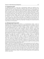
each of previous material models. This process (see Figure 1) is the first of the five stages
needed to manufacture a part that belongs to the fix system of the spare tire of a commercial
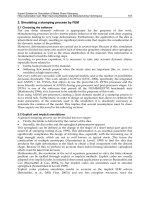
vehicle. Deformed blank obtained by this process is shown in Figure 2.

Fig. 1. Starting situation of the dies
Expert System for Simulation of Metal Sheet Stamping:
How Automation Can Help Improving Models and Manufacturing Techniques

143

Fig. 2. Deformed blank
The comparison between simulation results and the real deformed blank has been carried
out by means of a coordinate measuring machine. The dimension used to be compared
with simulation results is the stamping depth shown in Figure 3, and its real value is 15,88
mm.


Fig. 3. Stamping depth used to compare experimental and simulation results
Table 1 shows a comparison between results obtained by using the three material models.
For each model, several values of the main parameters have been tested. The maximum and
minimum value obtained as well as the averaged depth are displayed.

Model Minimum depth Averaged depth Maximum depth
Kinematic / Isotropic elastic
plastic model
15,82 mm 15,87 mm 15,92 mm
Strain rate dependent
isotropic plasticity model
15,68 mm 15,76 mm 15,85 mm
Piecewise linear isotropic
plasticity model
15,85 mm 15,90 mm 15,98 mm

Table 1. Comparison between material models
According to these results, and taking into account the real obtained depth (15,88 mm) it
can be concluded that any material model that has been considered in this study is
accurate enough to simulate the stamping process and the behavior of the involved
material.
However, the kinematic/isotropic elastic plastic model is the simplest one and the most
appropriate when the material behavior is not well known. Because of this, this model has
been adopted in the present work and is explained in the following section.
2.3.2 Kinematic / Isotropic elastic plastic model
This material model is described by the expresion Eq.(1) (Hallquist, 1998), based on the
Cowper- Symonds model (Cowper & Symonds, 1958, Dietenberger, et al., 2005, Jones, 1983),
which scales the yield stress by a strain rate dependent factor:

Expert Systems for Human, Materials and Automation

144

()
1
0
1
p
p
yp
e
ff
E
C
ε
σσβε

⎡⎤
⎛⎞
⎢⎥
=+ +
⎜⎟
⎢⎥
⎝⎠
⎢⎥
⎣⎦

(1)
Where:
0
σ
: Initial yield stress.
y
σ
: Yield stress.
ε

: Strain rate.
β
: Varying this parameter, isotropic ( 1
β
= ) or kinematic ( 0
β
= ) hardening can be
obtained. In this work, isotropic hardening is supposed, so
1
β

= .
p
E : Plastic hardening modulus, defined by Eq.(2), where
t
E
is the tangent modulus and E is
the elastic modulus:

t
p
t
EE
E
EE
=
−
(2)
p
eff
ε
: Effective plastic strain.
C and p: Strain rate parameters.
The following parameters have to be specified by the user in order to define properly this
material when using LS-DYNA. Those parameters are:
•
Density.
•
Young’s module.
•
Poisson ratio.

•
Initial yield stress.
•
Tangent modulus.
•
Hardening and strain rate parameters
β
, C and p.
2.4 Geometry of the dies and the blank
Finally, it is necessary to decide how to generate the geometry of the dies and the blank.
The forming tools are usually intended to impose the forming loads to the sheet metal
through the forming interface. In order to reduce computation time, only the surface of the
tooling has been included in the FEM model, rather than the complete geometry.
This is a common decision in sheet metal forming analysis (Firat, 2007a, c, Narasimhan &
Lovell, 1999), because of the fact that the forming tools should be, theoretically, designed to
be rigid and their deformation (that should be elastic with minimal shape changes) is
neglected.
The fact of defining dies as rigid bodies allows applying displacement restrictions in the
material definition.
The thickness defined for all the dies is 0.001mm, in order to distort the real geometry of the
contact faces as less as possible.
Regarding the sheet metal blank, because of its thin geometry, it is usually meshed with
shell elements (Darendeliler & Kaftanoglu, 1991, Firat, 2007a, c, Mattiasson, et al., 1995,
Narasimhan & Lovell, 1999, Taylor, Cao, Karafillis & Boyce, 1995, Tekkaya, 2000).
Expert System for Simulation of Metal Sheet Stamping:
How Automation Can Help Improving Models and Manufacturing Techniques

145
In this work, the reduced integration Belitschko-Tsay shell element (Belytschko, Liu &
Moran, 2000, Hallquist, 1998) has been used (included in the SHELL163 element

implemented in LS-DYNA). Five integration points have been defined through the thickness
in order to properly represent plasticity effects (Narasimhan & Lovell, 1999).
The Belitschko-Tsay shell element has proved to produce results that are similar to those
obtained with more complex elements and this element is the least expensive element
formulation of its kind (Firat, 2007a).
Contacts between the blank and the dies have been defined using an automatic surface-to-
surface contact algorithm and a static friction coefficient and a dynamic one are considered
during the simulation. With these two coefficients, the finite element simulation carries out a
thorough analysis of friction.
3. Developed application
3.1 Automation procedure
Every decision discussed above is aimed at achieving an application that automatically
generates the finite element model of a stamping process minimizing the user intervention.
The main steps of a FEM analysis can be resumed as follows (Álvarez- Caldas, 2009):
1.
Definition of analysis parameters (materials, loads…).
2.
Geometry creation.
3.
Analysis.
4.
Results post processing.
A different solution has been adopted to automate each one of them.
1.
Definition of analysis parameters: This is the hardest step for the user, and the one that
needs more automation. The designed application offers the user a window friendly
environment where all the parameters needed to define the simulation can be
introduced: blank thickness, material properties of the blank and the dies, loads,
restrictions, displacements, contact coefficients, simulation time… This windows
environment is programmed with Matlab Guide and generates a text file that can be

imported to LS-DYNA.
2.
Geometry creation: The user can generate the geometry entities for the blank and the
dies in any CAD program, exporting them to any graphic format that can be read by
LS-DYNA (as IGES).
3.
Analysis: All the parameters that have been introduced through the windows
environment, as well as the CAD geometries, have to be linked by the appropriate
ANSYS commands. The actions that must be done can be resumed as follows:
•
Import CAD geometry of the stamping tooling and the blank.
•
Creation and assignment of material models and real constants sets.
•
Definition of frictional contact conditions.
•
Description of forming process via the prescribed displacements or forces on the
tooling surfaces.
•
Meshing of the blank and the dies.
•
Resolution of the finite element model.
•
Since there are two kinds of potential users for this application (the ones that are
used to employ finite elements applications, and the ones that are not), two options
have been implemented:

Expert Systems for Human, Materials and Automation

146

• Blind analysis: All previous actions have been implemented in a generic
subroutine that is launched by the windows environment, so that all the
previous described process does not need user intervention.
•
Expert analysis: The automatic process ends before the solution step, allowing
the user to make any changes.
4.
Results post processing: this step cannot be automated because the user must be the one
to carry out the critical reviews of the results.
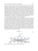
The proposed procedure is depicted in Figure 4, where stages that require user intervention
are drawn with solid line and those that can run “blindly” are drawn with broken line.


Fig. 4. Automation procedure
Once the proposed procedure is clear and taking into account that the automation may not
be done by someone non specialist in ANSYS LS-DYNA it is desirable to operate within a
friendly windows environment. In addition, the toolboxes available in some software such
as MATLAB are of great help. Therefore, a friendly windows environment has been
programmed in MATLAB by means of the GUI (Graphical User Interface) which is deeply
described in the following section.
3.2 Windows environment
By means of MATLAB’s GUI a friendly window environment has been designed in order to
provide the user a step by step procedure that ensures the correct operations that must be
done in the finite element model which simulates the stamping process. The proposed
environment generates a set of files which is afterwards forwarded automatically by the
software to ANSYS LS-DYNA so that it runs in batch mode, that is, under system without
having to involve the user in the modelling of the stamping process. In addition, the
proposed environment carries out an estimation loop so as to predict the values of the
material parameters that best fit the model with experimental test results. Therefore, the
software which has been developed allows the user either to simulate a stamping process or

to find the material parameters that best suit the stamping process. In Figure 5 the window
that allows simulating a stamping process is depicted.
Expert System for Simulation of Metal Sheet Stamping:
How Automation Can Help Improving Models and Manufacturing Techniques

147

Fig. 5. Window environment of the developed software


Fig. 6. Specifying the material properties of the blank

Expert Systems for Human, Materials and Automation

148
This part of the software is divided in three steps. In the first step the user must select the
plasticity material model that best describes the material used as a blank. Figure 6 shows the
parameters to be introduced by the user if an isotropic hardening plasticity model is selected
to model the blank.
In addition, the user has to introduce the thickness of the blank, the meshing size and has to
load the “*.iges” file that contains the blank geometry. Afterwards, the user must specify in
the second step the number of steps in which the stamping process will be done, as well as
other parameters such as the maximum number of dies which will be used during the
process, etc. Finally, in the third step the properties of the dies employed during the
stamping, including the die material properties (see Figure 7) and load vectors are applied.
During the clicking of each of the buttons certain files are being generated automatically
which will finally be the input to ANSYS LS-DYNA. In addition, the software allows
distinguishing between users that have previous experience in ANSYS LS-DYNA by
clicking in the simulation options button. Once clicked, the user can specify the simulation
time or either open LS–DYNA in order to load the simulation and allow changes in the

model before running the solution.



Fig. 7. Specifying the material properties of the die
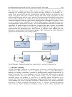
One of the problems that may be encountered is that the values of material parameters are
not known and therefore have to be adjusted before simulating the complete stamping
process. To solve this problem the following steps are proposed:
Expert System for Simulation of Metal Sheet Stamping:
How Automation Can Help Improving Models and Manufacturing Techniques

149
• In the first place the user must select a certain manufacturing process to be simulated.
•
Afterwards, this process will be carried out in an industry using the available dies and
devices. This test will be defined as a pattern test.
•
Thirdly, the pattern test will be done in the material whose parameters want to be
computed. Due to the fact that the selected process is well known and defined, all the
changes that take place in the final shape will be due to changes in material
properties.
•
Finally, once the material parameters have been clearly found other processes may be
simulated once the optimum material parameters are known. This information may be
used for designing new dies for new upcoming processes saving money and time as the
number of experimentally tested dies has decreased a lot.
3.3 Estimation of material parameters
In order to adjust the material parameters the designed software provides a specific tool that
compares the results of the finite element simulation with the results of a real experimental
test (Gauchía, 2009). The user must specify at least two sets of simulations where the values

of the material parameters are different. The software will create the files needed to carry
out the finite element model and return a solution which will be compared with the
experimental test results given by the user. From two simulations, the software provides by
means of a linear interpolation an estimation of the material parameters. Because the
provided values are the result of a linear interpolation the proposed material parameters
may not be the most appropriate. Therefore, the user can modify the proposed values and
carry out a third simulation. Once the results of this third simulation are provided the
software shows different graphs that show the results obtained in the previous simulations
for each of the material parameters. If for example, the depth is considered as the result to be
compared with the experimental tests the prediction plots display graphs where each of the
material properties is represented in the vertical axis and the depth in the horizontal axis. In
addition, the user may modify the polynomial degree (linear, quadratic, etc.) for the
simulated results. These graphs, represented inFigure 8, display the polynomial function
and confidence bounds. Each of the results are plotted in the polynomial fit estimation and
represented as a cross (“+”).
The proposed software allows carrying out more than three simulations. If the user does
more simulations the confidence bounds will narrow, however, the user will have to find
the proper balance between computation time and exactness. It must also by noted that
only some of the most sensitive material parameters can be changed by the user, as
depicted in Figure 9. The material parameters the user is allowed to change are the yield
stress, parameter C and parameter p of the plasticity model. The yield stress is without
doubt one of the most important parameters that characterize the plasticity material
model. Previous simulations (Quesada, et al., 2009) have shown that variations of
approximately 14% in the depth may be encountered. However, it was found that
parameters C and p do not have a great influence in the results. Previous simulations
revealed that varying parameter C a 900%, produces a variation of less than 0.5% in the
result and varying parameter p a 133% produces a variation of 0.4% in the final result.
Therefore, the influence of other parameters can be neglected and will not be considered
during the material parameter estimation.

Expert Systems for Human, Materials and Automation

150



Fig. 8. Polynomial fit estimation and confidence bounds of material parameters




Fig. 9. Material parameters that can be modified by the user
Expert System for Simulation of Metal Sheet Stamping:
How Automation Can Help Improving Models and Manufacturing Techniques

151

Fig. 10. Material parameters estimation procedure
4. Application example
4.1 Choosing and simulating the pattern test
The first step is choosing the pattern test. For a stamping process, the example explained in
2.3.4 has been chosen. As stated before, this test is the first of the five stages needed to
manufacture a part which belongs to the fix system of the spare tire of an real vehicle. The
parts involved in this step are shown in Figure 11:

Expert Systems for Human, Materials and Automation

152

Fig. 11. First step dies

The blank is leaned on the bed die and the process starts with the movement of the
blankholder, which applies a load to hold the blank once contact is established between them.
After that, punch begins to go down, deforming the blank to obtain the part shown in Figure 2.
Deformed blank was measured with a coordinate measuring machine, and the dimension
used to be compared with simulation results is shown in Figure 3. Simulation displacements
are compared with real ones because displacement measurement assures a controlled final
shape of the sheet blank. Other variables such as stress or strains are not useful from a
practical point of view for this purpose.
Every parameter involved in this simulation has to be adjusted according to the designer
experience and taking into account the conditions of the experimental stamping process
(loads, times, boundary conditions ). Boundary and loading conditions have been specified
by fixing degrees of freedom of the dies or by aplying displacements and loads to them to
simulate the real process (Table 2).

Time [s]
Punch displacement
[mm]
Blankholder
displacement [mm]
Blankholder load
[N]
0 0 0 0
0,5 -38 -25 -90000
1 -78,5 -49,998 -90000
1,5 -116,498 -49,998 -90000
2 -78,5 -49,998 -90000
2,5 -38 -25 -90000
3 0 0 0
Table 2. Loads and displacements used in the pattern test simulation
Those parameters are introduced in the friendly windows environment exposed in chapter

3.2, and the stamping process is automatically simulated by ANSYS LS-DYNA according to
the procedure shown in Figure 4.
As long as the patters test is well known and the real experiment can be carried out for any
desired material, simulation results can always be compared with experimental values and
simulation parameters can be adjusted in order to obtain a validated model.
Expert System for Simulation of Metal Sheet Stamping:
How Automation Can Help Improving Models and Manufacturing Techniques

153
4.2 Adjusting material parameters for a high strength steel
Once the pattern test can be simulated with great confidence, it is time to use it to adjust
parameters of an unknown material in order to optimize results, predict springback and
define new dies before carrying out the experimental test.
The material parameter estimation procedure needs two sets of material parameters to start.
The program simulates the pattern test with these two sets and the difference between
experimental and simulation results is calculated. If this difference is over the tolerance limit
specified by the user, the application founds new material parameters by applying linear
interpolation to previous ones and launches a new simulation with these new material
parameters. The process is repeated until results fit tolerance requirements.
In the experimental test, the displacement of the punch is 16.5 mm. For this value, the final
depth of the manufactured part, measured by the MMC machine, is 15.9 mm.
Initial values for the material parameters and the depths obtained for each combination can
be seen in Table 3 (1
st
and 2
nd
simulations). The last column shows the parameters values
obtained after optimization, considering a tolerance limit for the relative error of 0.4%.

Number of simulation

Parameter
1st 2nd
Last
Density (kg/m
3
) 7800 7800 7800
Young’s module (MPa) 210000 210000 210000
Poisson ratio 0.3 0.3 0.3
Yield stress (MPa) 354 425 664
Tangent modulus (MPa) 763 763 763
β

1 1 1
C (s
-1
) 40 100 10.99
p 5 5 2.5
Obtained depth (mm) 16.14 16.14 15.96
Relative error 1.5% 1.5% 0.38%
Table 3. Employed parameters
4.3 Results validation
To validate these results, obtained parameters have been used in a new deep stamping
process. The selected test covers steps 1, 2 and 3 of the manufacture process of the part
shown in Figure 12.


Fig. 12. Manufactured part

Expert Systems for Human, Materials and Automation

154
This process involves not only geometrical difficulty but also difficulties due to progressive
stamping processes. The first step is the pattern test explained in 4.1. Dies used in steps 2
and 3 are shown in Figure 13.


Fig. 13. Second and third steps dies
In this case, the dimension used to validate de model is the one shown in Figure 14. This
dimension achieved a value of 77.21 mm in the experimental test after springback.
Simulation result was 74.58 mm, representing a 3.4% error.


Fig. 14. Final dimension used for validation
5. Adaptive meshing
It has been mentioned before that computing time becomes an important aspect in this kind
of simulations. To solve the developed models, a PC can take from several hours to a week,
depending mainly on the mesh size and on the amount of plastic strain reached. Mesh size
is critical not only for the results quality but for taking into account properly contact
between parts. High relative speed between dies characteristic of stamping processes makes
necessary to use fine mesh sizes and high contact stiffness, both of them leading to increase
computational load.
In addition, to repeat many times the early steps of a multistep process is needed to adjust
properly the mesh size in order to get an acceptable going of the latest steps. It multiplies at
the same time programming and computing times. In this context, Numeric Calculation
Adaptive Meshing (AM) technique is of paramount importance.
Using the AM tool will allow the stress analyst to save because:
•
It is not needed to carry out meshing tests. An initial gross mesh can be provided, and
in the first calculation it will be automatically refined in those areas in which strains
Expert System for Simulation of Metal Sheet Stamping:

How Automation Can Help Improving Models and Manufacturing Techniques

155
grow higher. It won’t be necessary to have a prediction about the areas that are going to
need remeshing neither the remeshing level. Resources are disposed at the time they are
required.
•
It won’t be necessary to provide, for the early steps of the process, a refined mesh in the
areas that are going to experiment high strain levels in the last steps. It avoids the
calculation in these early steps to be unnecessarily heavy.
5.1 Adaptive meshing tool in LS-DYNA
LS-DYNA (LSTC, 1998) includes an h-adaptive method for the shell elements (Belytschko, et
al., 1989). In an h-adaptive method, the elements are subdivided into smaller elements
wherever an error indicator shows that subdivision of the elements will provide improved
accuracy. The beginning objective of the adaptive process used in LS-DYNA is to obtain the
greatest accuracy for a given set of computational resources. The user sets the initial mesh
and the maximum level of adaptivity, and the program subdivides those elements in which
the error indicator is the largest. Although this does not provide control on the error of the
solution, it makes it possible to obtain a solution of comparable accuracy with fewer
elements, and, hence, less computational resources, than with a fixed mesh.
The original mesh provided by the user is known as the parent mesh, the elements of this
mesh are called the parent elements, and the nodes are called parent nodes. Any elements
that are generated by the adaptive process are called descendant elements, and any nodes
that are generated by the adaptive process are called descendant nodes. Elements generated
by the second level of adaptivity are called first-generation elements, those generated by
third level of adaptivity are called second-generation elements, etc. The coordinates of the
descendant nodes are generated by using linear interpolation.
Refinement indicators are used to decide the locations of mesh refinement. One deformation
based approach checks for a change in angles between contiguous elements.
5.2 Adaptive meshing programming in LS-DYNA

EDADAPT command activates AM for a part of the simulation. It should be applied to
blank parts, since dies are modeled as rigid and no strains or stresses are calculated into
dies. The mesh size of rigid dies can be as fine as desired because it does not imply
additional calculations. For example, to activate AM for PART #1 the following command
must be written:
EDADAPT, 1, ON
AM activation command is placed just before SOLVE command, and does not modify any
other programming structure, which makes possible an easy incorporation to the
automation scheme described in previous sections.
5.3 Adaptive meshing controls
Adaptive Meshing control parameters have to be defined by means of EDCADAPT
command. These parameters are defined just below (ANSYS, 2005):
•
FREQ- Time interval between adaptive mesh refinements.
•
TOL- Adaptive angle tolerance (in degrees) for which adaptive meshing will occur.
If the relative angle change between elements exceeds the specified tolerance value,
the elements will be refined.

• OPT- Adaptivity option:

Expert Systems for Human, Materials and Automation

156
• 1. Angle change (in degrees) of elements is based on original mesh configuration.
• 2. Angle change (in degrees) of elements is incrementally based on previously
refined mesh.

• MAXLVL- Maximum number of mesh refinement levels. This parameter controls
the number of times an element can be remeshed. Values of 1, 2, 3, 4, etc. allow a

maximum of 1, 4, 16, 64, etc. elements, respectively, to be created for each original
element.

• BTIME/DTIME- Birth/Death time to begin/end adaptive meshing. It controls
when AM is activated/deactivated

• LCID- Data curve number identifying the interval of remeshing. The abscissa of
the data curve is time, and the ordinate is the varied adaptive time interval. If LCID
is nonzero, the adaptive frequency (
FREQ) is replaced by this load curve. Note that
a nonzero
FREQ value is still required to initiate the first adaptive loop.
• ADPSIZE- Minimum element size to be adapted based on element edge length.
• ADPASS- One or two pass adaptivity option:
• 0. Two pass adaptivity. Results are recalculated after remeshing.
• 1. One pass adaptivity. Results are not recalculated after remeshing.
• IREFLG- Uniform refinement level flag. Values of 1, 2, 3, etc. allow 4, 16, 64, etc.
elements, respectively, to be created uniformly for each original element.

• ADPENE- Adaptive mesh flag for starting adaptivity when approaching (positive
ADPENE value) or penetrating (negative ADPENE value) the tooling surface. Adaptive
tool refinement is based on the tool curvature.
•
ADPTH- Absolute shell thickness level below which adaptivity should begin. This
option works only if the adaptive angle tolerance (
TOL) is nonzero. If thickness based
adaptive remeshing is desired without angle change, set
TOL to a large angle.
•
MAXEL- Maximum number of elements at which adaptivity will be terminated.

Adaptivity is stopped if this number of elements is exceeded.
Adaptive Meshing used to simulate stamping processes has shown to work properly with
the combination of control parameters revealed below:
EDCADAPT,0.1,0.5,2,3,0,1 , ,0,0,0,0,0,0,
Which means:
FREQ=0.1; TOL=0.5; OPT=2; MAXLVL=3; BTIME=0; DTIME=1.
These values can vary from one simulation to another.
5.4 Computing time saving
The 2-step stamping process analyzed in section 4 has been carried out with and without
AM option, in the same computer, reaching very similar results in both cases.
In the case fine mesh is programmed from the beginning of the calculation, first step took 50
hours and second step 70 hours; 120 hours to complete the entire calculation.
In the case AM is programmed (Figure 15) over a gross initial mesh, 10 hours have been
taken to complete calculation.
Additionally, these times does not take account of the efforts made by the stress analyst to
find the appropriate mesh density for each blank area as a function of the final plastic
strain.
Expert System for Simulation of Metal Sheet Stamping:
How Automation Can Help Improving Models and Manufacturing Techniques

157

Fig. 15. Evolution of the adaptive mesh in step one simulation
5.5 Problems encountered during adaptive meshing implementation
As has been shown in section 2.2, combined “Explicit to Implicit” simulations have resulted
to be the most appropriate way to simulate the complete stamping process, using Full
Restart option to concatenate different stamping steps. However, ANSYS Release 10.0
Documentation says textually:
“Adaptive meshing: Adaptive meshing (EDADAPT and EDCADAPT) is not supported in a
full restart. In addition, a full restart is not possible if adaptive meshing was used in the

previous analysis. “(ANSYS, 2005)
So it can be concluded that using LS-DYNA AM tool to simulate a multistep stamping
process forces the stress analyst to develop a unique Explicit procedure, programming
different dies approximation and retiring in the same calculation.
6. Conclusions
According with previous expositions and results, it can be concluded:
•
A procedure to simulate real sheet metal forming processes by means of finite elements
has been established.
•
To define this procedure, several options have been analyzed for each step of the
process, choosing the one more suitable between the possibilities offered by finite
elements software.
•
Such a procedure has been automated and allows performing simulations with no user
intervention, avoiding the difficulty of using a high-level program as LS-DYNA.
•
By means of this automated procedure a methodology to adjust material parameters
has been developed.
•
Parameters involved in each material model have been identified and their influence in
final results has been quantified. This is very useful to fit material properties in other
simulations.
•
This methodology is based in real experimental and simulation results and in a material
parameter fit estimation procedure.
•
Real industry experimental tests to validate the simulation results, instead of
benchmark theoretical tests, have been carried out. This allows to use previous
knowledge of the designer, to particularize material characterization for each kind of

process and avoids building specific tooling.
•
Simulation model has been validated by comparing its results with those obtained in
experimental tests. An example of a real application of the industry has been presented.

Expert Systems for Human, Materials and Automation

158
• LS-DYNA adaptive meshing has been also tested. Results obtained by using it are
virtually the same as those validated before and time is greatly reduced. So, it can be
conclude that using adaptive meshing highly recommended.
•
Using adaptive meshing forces to avoid implicit simulations in springback estimation.
Therefore, a complete explicit simulation of the application and withdrawal of dies
must be carried out.
7. Acknowledgment
The authors want to thank ARRAN Automoción Group for its great interest and
collaboration in this work and the Government of Spain for the support given through the
project 370100-103 of the PROFIT program.
8. References
Álvarez- Caldas, C., et al. (2009). Expert System for Simulation of Metal Sheet Stamping.
Engineering with computers, Vol. 25, No. 4, pp. 405- 410. ISSN 0177-0667.
ANSYS (2005).
ANSYS LS- DYNA User's Guide. ANSYS release 10.0. ANSYS Inc. Canonsburg,
USA.
Belytschko, T., et al. (1989). Fission - Fusion Adaptivity in Finite Elements for Nonlinear
Dynamics of Shells.
Computers and Structures, Vol. 33, No. pp. 1307- 1323, ISSN
Buranathiti, T.&Cao, J. (2005a). Numisheet2005 Benchmark Analysis on Forming of an
Automotive Deck Lid Inner Panel: Benchmark 1,

NUMISHEET 2005: Proceedings of
the 6th International Conference and Workshop on Numerical Simulation of 3D Sheet
Metal Forming Process. AIP Conference Proceedings
, Detroit, Michigan, USA, 15-
19/08/2005.
Buranathiti, T.&Cao, J. (2005b). Numisheet2005 Benchmark Analysis on Forming of an
Automotive Underbody Cross Member: Benchmark 2,
NUMISHEET 2005:
Proceedings of the 6th International Conference and Workshop on Numerical Simulation of
3D Sheet Metal Forming Process. AIP Conference Proceedings
, Detroit, Michigan, USA,
15-19/08/2005.
Cowper, G. R.&Symonds, P. S. (1958).
Strain Hardening and Strain Rate Effects in the Impact
Loading of Cantilever Beams
. Brown University. Providence, Rhode Isl, USA.
Chen, M. H., et al. (2007). Application of the forming limit stress diagram to forming limit
prediction for the multi-step forming of auto panels.
Journal of Materials Processing
Technology
, Vol. 187-188, No. pp. 173-177, ISSN 0924-0136
Darendeliler, H.&Kaftanoglu, B. (1991). Deformation Analysis of Deep-Drawing by a Finite
Element Method.
CIRP Annals - Manufacturing Technology, Vol. 40, No. 1, pp. 281-
284, ISSN 0007-8506
Dietenberger, M., et al. (2005). Development of a High Strain-Rate Dependent Vehicle
Model,
4th LS-DYNA Forum, Bamberg, Germany 20th - 21st of October 2005.
Firat, M. (2007a). Computer aided analysis and design of sheet metal forming processes: Part
I - The finite element modeling concepts.

Materials & Design, Vol. 28, No. 4, pp.
1298-1303, ISSN 0261-3069
Firat, M. (2007b). Computer aided analysis and design of sheet metal forming processes:
Part II - Deformation response modeling.
Materials & Design, Vol. 28, No. 4, pp.
1304-1310, ISSN 0261-3069
Expert System for Simulation of Metal Sheet Stamping:
How Automation Can Help Improving Models and Manufacturing Techniques

159
Firat, M. (2007c). U-channel forming analysis with an emphasis on springback deformation.
Materials & Design, Vol. 28, No. 1, pp. 147-154, ISSN 0261-3069
Gau, J T. (1999).
A Study of the Influence of the Bauschinger Effect on Springback in Two-
Dimensional Sheet Metal Forming
. Ph.D. Degree. The Ohio State University. Ohio.
Gauchía, A. et al. (2009). Material parameters in a simulation of metal sheet stamping.
Proceedings of the Institution of Mechanical Engineers Part D-Journal of Automobile
Engineering.
Vol. 223. No. 6, pp. 783- 791. ISSN 0954-4070.
Hallquist, J. O. (1998).
LS-DYNA Theoretical Manual. LSTC. Livermore, California, USA.
Ling, Y. E., et al. (2005). Finite element analysis of springback in L-bending of sheet metal.
Journal of Materials Processing Technology, Vol. 168, No. 2, pp. 296-302, ISSN 0924-
0136
LSTC (1998).
LS-DYNA Theoretical Manual. Livermore Software Technology Corporation.
Livermore, California, USA.
LSTC (2006).
LS-DYNA: User's Manual Version 971. Livermore Software Technology

Corporation. Livermore, California, USA.
Makinouchi, A. (1996). Sheet metal forming simulation in industry.
Journal of Materials
Processing Technology
, Vol. 60, No. 1-4, pp. 19-26, ISSN 0924-0136
Mattiasson, K., et al. (1995). Simulation of springback in sheet metal forming,
Proceedings of
the NUMIFORM’95 Simulation of Materials Processing: Theory, Methods and
Applications
, Cornell University, Ithaca, NY, USA,
Morestin, F., et al. (1996). Elasto plastic formulation using a kinematic hardening model for
springback analysis in sheet metal forming.
Journal of Materials Processing
Technology
, Vol. 56, No. 1-4, pp. 619-630, ISSN 0924-0136
Narasimhan, N.&Lovell, M. (1999). Predicting springback in sheet metal forming: an explicit
to implicit sequential solution procedure.
Finite Elements in Analysis and Design, Vol.
33, No. 1, pp. 29-42, ISSN 0168-874X
Ortiz, M.&Quigley, J. J. (1991). Adaptive mesh refinement in strain localization problems.
Computer Methods in Applied Mechanics and Engineering, Vol. 90, No. 1-3, pp. 781-804,
ISSN 0045-7825
Quesada, A., et al. (2009). Influence of the parameters of the material model in finite element
simulation of sheet metal stamping,
7th EUROMECH Solid Mechanics Conference,
Lisbon (Portugal), September, 7th- 11th, 2009.
Quigley, E.&Monaghan, J. (2002). Enhanced finite element models of metal spinning.
Journal
of Materials Processing Technology
, Vol. 121, No. 1, pp. 43-49, ISSN 0924-0136

Samuel, M. (2004). Numerical and experimental investigations of forming limit diagrams in
metal sheets.
Journal of Materials Processing Technology, Vol. 153-154, No. pp. 424-
431, ISSN 0924-0136
Silva, M. B., et al. (2004). Stamping of automotive components: a numerical and
experimental investigation.
Journal of Materials Processing Technology, Vol. 155-156,
No. pp. 1489-1496, ISSN 0924-0136
Song, J H., et al. (2007). A simulation-based design parameter study in the stamping process
of an automotive member.
Journal of Materials Processing Technology, Vol. 189, No. 1-
3, pp. 450-458, ISSN 0924-0136
Taylor, L., et al. (1995). Numerical simulations of sheet-metal forming.
Journal of Materials
Processing Technology
, Vol. 50, No. 1-4, pp. 168-179, ISSN 0924-0136

Expert Systems for Human, Materials and Automation

160
Tekkaya, A. E. (2000). State-of-the-art of simulation of sheet metal forming. Journal of
Materials Processing Technology
, Vol. 103, No. 1, pp. 14-22, ISSN 0924-0136
Wei, L.&Yuying, Y. (2008). Multi-objective optimization of sheet metal forming process
using Pareto-based genetic algorithm.
Journal of Materials Processing Technology, Vol.
208, No. 1-3, pp. 499-506, ISSN 0924-0136

9
Expert System Used on Materials Processing

Vizureanu Petrică
“Gheorghe Asachi” Technical University Iasi,
Romania
1. Introduction
Conventional computing programs characterize through an algorithm approach as the
specialists called it. This approach allows solving a problem by using a preset computing
scheme which applies to some structures well-known for input information and produces a
result that keep to program operations sequence made within computing scheme. Yet, there
is another category of problems whose solving has nothing to do with classic algorithms but
supposes a higher volume of specialty knowledge for very strait domains. Such specialty
knowledge does not represent the usual “luggage” of a certain human subject, they being on
view only for experts within the interest domain of the problem. Such problems can treat
subjects as automat diagnosis, monitoring, planning, design or technical scientific analysis.
Computing programs that solves such problems are known as expert systems (ES) and the
first development attempts of such programs dates from mid of 1960 – 1970’s. Unlike
conventional programs, ES are conceived to use, mainly, symbolic sentence, developed
through interference. As a branch of artificial intelligence (AI), expert systems developed
pursuing the study of knowledge processing.
An expert system is a program that uses knowledge and interference procedures for solving
quite difficult problems, which normally needs the intervention of a human expert to find
the solution. Shortly, expert systems are programs that store specialty knowledge inserted
by experts.
2. Characteristics of ES
These systems are often used under situations without a clear algorithmic solution. Their
main characteristic is the presence of a knowledge base along with a search algorithm
proper to the reasoning type. Knowledge base is very large most times, so the way of
representing knowledge is very important. Knowledge base of the system must separate
from the program, which must be as stable as possible. The most used way of
representing knowledge is a multitude of production rules. Operations of these systems
are further controlled by a simple procedure whose nature depends on knowledge nature.

As in other artificial intelligence programs, when other techniques are not available,
search has recourse to. Expert systems built up to date differs from this point of view. The
question arises whether there can be written rules as strict as in any situation there is only
an applicable solution? And, also, finding all solutions is necessary or it is sufficient only
one?

Expert Systems for Human, Materials and Automation

162
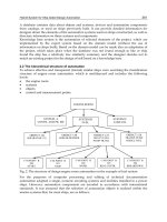
An expert system must have compulsory three main modules that form the so-called
essential system:
• Knowledge base formed by the assembly of specialized knowledge introduced by
human expert. The knowledge stored here is mainly objective descriptions and the
relations between them; knowledge base takes part from the cognitive system,
knowledge being memorized into a specially organized space; storage form must assure
the search of knowledge pieces specified directly through identifying symbols or
indirect through associated properties or interferences that start from other knowledge
pieces.
• Interference engine represents the novelty of expert system and takes over from
knowledge base the fact used for building reasoning. Interference engine pursues a
series of major objectives such as control strategy election based on current problem,
elaboration of the plan that solves the problem after necessities, switching from a
control strategy to another one, execution of the actions preset in solving plan.
Although interference mechanism is built from a procedures assembly in the usual
meaning of the term, the way in which knowledge are used is not estimated by
program but depends on the knowledge it has at command.
• Facts base represents an auxiliary memory that contains all users’ data (initial facts that
describe the source of the solving problems) and the intermediary results made during
reasoning. The content of the facts base is stored generally in volatile memory (RAM)
but to user request; it can be stored on hard disk.

2.1 The modules of an ES
Communication module assures specific interfaces for users and for knowledge acquisition.
User interface allows the dialogue between user and quasi natural language system. It
transmits to interference mechanism user’s requests and his results. It facilitates equally the
acquisition of the initial problem and result communication.


Fig. 1. ES modules

Expert System Used on Materials Processing

163
Acquisition module of knowledge takes specialized knowledge given by human expert
through the engineer, into a not specific form to intern representation. A series of
knowledge can arise as files specific to databases or to other external programs. This module
receives the knowledge, verifies their validity and finally generates a coherent knowledge
base.
Explaining module allows path tracing followed in reasoning process by resolvent system
and explanation issuance for the achieved solution by emphasizing the causes of eventual
mistakes or the reason of a failure. It helps the expert to verify the consistency of the
knowledge base.
Explanation and updating. In terms of the application that it is built for, the effective
structure of an expert system can differ towards the standard structure.
For example, initial data can be acquired from the user and from automatic control
equipment
Nevertheless, it is important for expert systems to have two characteristics:
• To explain the reasoning and if it is not possible, human users could not accept it. For
this, it must be enough meta-knowledge for explanations and the program must go in
intelligible steps.
• To attain new knowledge and to modify the old ones, and usually the only way of

introducing knowledge into an expert system is by human expert interaction.
2.2 Development of an ES
The development of an expert system represents design process of the system going from users’
demands of implementing testing and finally launching the product onto market for the
effective use. Many times, there are distinctions in design stage between physical design and
logical one because these stages need different activities and resources both technological
nature and human one.


Fig. 2. Physical design.
Physical design includes the design of hardware resources and knowledge base, which
includes acquisition components of the knowledge and representation way. When physical
part is design sub-systems are appropriate implemented and tested. Only afterwards, they
can be tested together with logical part.

Expert Systems for Human, Materials and Automation

164
Logic design refers to software design and realizes parallel to physical one. First, assembly
decisions take such as those linked to the election of a programming language or a shell or a
toolkit. Both integration problems of the system and security ones must solve. Then
interference engine and interfaces are designed. To program interference engine declarative
languages are chosen several times. The design of this part of the system can be seen as an
activity of software development, as programming engineering says. The particularity of ES
is the importance and development of the knowledge base.
In addition, the exclusive accent is not put on developing interference engine program but
on developing the other component such as interfaces.
Each subsystem could need different resources (other programming languages or even other
hardware resources) and distinct development techniques.
2.3 ES advantages

• They are valuable collections of information
• They are indispensable without human expertise
• In some situation, they can be cheaper and more effective than human experts can
• They can be faster than human experts can
• If flexible, they can be easily up-dated
• They can be used to instruct new human experts
• At request, they can explain the premises and reasoning line.
• They treat the uncertainty into an explicit manner, which, unlike human experts, can be
verified.


Fig. 3. Logic design.
3. Stages in the design and implementation of an ES
Expert systems are, in fact, particular cases of the production systems, which address to some
domains with a very strait specialization. In fact, the larger the number of knowledge within
a system is the efficient it acts. As human expert, ES has a sphere of competences limited
only to a certain domain, usually, very strait, its functionality lying on the human reasoning
pattern: starting from certain knowledge or facts, ES develops a series of interferences and
reaches to a certain conclusion. Under the context, a synthetic definition of ES would be as
follows programs dedicated usually to a specific domain that try to emulate human experts’ behavior.

Expert System Used on Materials Processing

165

Fig. 4. ES implementation.
• They cannot reason based on intuition or common sense because they cannot be easily
representable
• They are limited to a restrained domain; knowledge from other domains cannot be
easily integrated nor cannot generalize convincingly

• Learning process is not automate; in order to up-date knowledge it is needed human
intervention
• Nowadays, they cannot reason based on theories and analyses
• The knowledge stored in knowledge base depend very much on the human expert that
express and articulate them
As a component of production systems, ES is one of the most used patterns for representing
and control of knowledge. Within this terminology, the word production must not be
confounded with which happens in factories and plants. Its significance can be translated
according to the definition as the production of new facts added into knowledge base due to
the appliance of these rules. A possible definition of the production system including ES
referring to their structure could comprise the following elements:
• A set of rules, each rule has two components such as component condition that
determines when the rule applies and component consequence that describes the action,
which results by applying the rule. This set of rules form rules base.
• One or many databases contain the information describing the analyzed problem. This
database contains initial information where new facts add resulted by applying the
rules. This set of information forms facts base.
• A control mechanism or rules interpreter frequently named interference engine, which
assures the stability of rules appliance order for the existent database. The selection of
the rule that applies and solve the appeared conflicts when many rules can be applied
simultaneously.
• Communication between operator and ES accomplishes by a specialized interface that
assures the efficient exploitation and development of the ES. This interface allows the
achievement of two important functions such as:
a. On one hand, at human operator demand ES can explain the reasoning it achieved.
This is necessary because as complex and “praised” ES is, human operator cannot
always accept “blindly” the solution proposed by ES but he wants to pursue and
analyze the reasoning machine made.
b. On the other hand, in order ES develop by gathering experience it is necessary the
modification of the old knowledge and addition of new ones into knowledge base.