Heat Analysis and Thermodynamic Effects Part 1 ppt

HEAT ANALYSIS AND
THERMODYNAMIC EFFECTS

Edited by Amimul Ahsan













Heat Analysis and Thermodynamic Effects
Edited by Amimul Ahsan


Published by InTech
Janeza Trdine 9, 51000 Rijeka, Croatia

Copyright © 2011 InTech
All chapters are Open Access articles distributed under the Creative Commons
Non Commercial Share Alike Attribution 3.0 license, which permits to copy,
distribute, transmit, and adapt the work in any medium, so long as the original
work is properly cited. After this work has been published by InTech, authors
have the right to republish it, in whole or part, in any publication of which they
are the author, and to make other personal use of the work. Any republication,

referencing or personal use of the work must explicitly identify the original source.

Statements and opinions expressed in the chapters are these of the individual contributors
and not necessarily those of the editors or publisher. No responsibility is accepted
for the accuracy of information contained in the published articles. The publisher
assumes no responsibility for any damage or injury to persons or property arising out
of the use of any materials, instructions, methods or ideas contained in the book.

Publishing Process Manager Marija Radja
Technical Editor Teodora Smiljanic
Cover Designer Jan Hyrat
Image Copyright 2happy, 2010. Used under license from Shutterstock.com

First published September, 2011
Printed in Croatia

A free online edition of this book is available at www.intechopen.com
Additional hard copies can be obtained from



Heat Analysis and Thermodynamic Effects, Edited by Amimul Ahsan
p. cm.
ISBN 978-953-307-585-3

free online editions of InTech
Books and Journals can be found at
www.intechopen.com

Contents

Preface IX
Part 1 Thermodynamic and Thermal Stress 1
Chapter 1 Enhancing Spontaneous Heat Flow 3
Karen V. Hovhannisyan and Armen E. Allahverdyan
Chapter 2 The Thermodynamic Effect of Shallow
Groundwater on Temperature
and Energy Balance at Bare Land Surface 19
F. Alkhaier, G. N. Flerchinger and Z. Su
Chapter 3 Stress of Vertical Cylindrical Vessel for
Thermal Stratification of Contained Fluid 39
Ichiro Furuhashi
Chapter 4 Axi-Symmetrical Transient Temperature Fields and
Quasi-Static Thermal Stresses Initiated by a Laser
Pulse in a Homogeneous Massive Body 57
Aleksander Yevtushenko, Kazimierz Rozniakowski

and Malgorzata Rozniakowska-Klosinska


Chapter 5 Principles of Direct Thermoelectric Conversion 93
José Rui Camargo and Maria Claudia Costa de Oliveira
Chapter 6 On the Thermal Transformer Performances 107
Ali Fellah and Ammar Ben Brahim

Part 2 Heat Pipe and Exchanger 127
Chapter 7 Optimal Shell and Tube Heat Exchangers Design 129
Mauro A. S. S. Ravagnani, Aline P. Silva and Jose A. Caballero
Chapter 8 Enhancement of Heat Transfer in the
Bundles of Transversely-Finned Tubes 159
E.N. Pis’mennyi, A.M. Terekh and V.G. Razumovskiy
VI Contents

Chapter 9 On the Optimal Allocation of the Heat
Exchangers of Irreversible Power Cycles 187
G. Aragón-González, A. León-Galicia and J. R. Morales-Gómez
Part 3 Gas Flow and Oxidation 209
Chapter 10 Gas-Solid Flow Applications for Powder Handling
in Industrial Furnaces Operations 211
Paulo Douglas Santos de Vasconcelos and
André Luiz Amarante Mesquita
Chapter 11 Equivalent Oxidation Exposure - Time for Low
Temperature Spontaneous Combustion of Coal 235
Kyuro Sasaki and Yuichi Sugai
Part 4 Heat Analysis 255
Chapter 12 Integral Transform Method Versus Green Function
Method in Electron, Hadron or Laser Beam -
Water Phantom Interaction 257
Mihai Oane, Natalia Serban and Ion N. Mihailescu
Chapter 13 Micro Capillary Pumped Loop for Electronic Cooling 271
Seok-Hwan Moon and Gunn Hwang
Chapter 14 The Investigation of Influence Polyisobutilene Additions
to Kerosene at the Efficiency of Combustion 295
V.D. Gaponov, V.K. Chvanov, I.Y. Fatuev,
I.N. Borovik, A.G. Vorobiev, A.A. Kozlov, I.A. Lepeshinsky,

Istomin E.A. and Reshetnikov V.A
Chapter 15 Synthesis of Novel Materials by
Laser Rapid Solidification 313
E. J. Liang, J. Zhang and M. J. Chao
Chapter 16 Problem of Materials for Electromagnetic Launchers 321
Gennady Shvetsov and Sergey Stankevich
Chapter 17 Selective Catalytic Reduction NO by Ammonia Over
Ceramic and Active Carbon Based Catalysts 351
Marek Kułażyński










Preface

The heat transfer and analysis on heat pipe and exchanger, and thermal stress are
significant issues in a design of wide range of industrial processes and devices. This
book introduces advanced processes and modeling of heat transfer, gas flow,
oxidation, and of heat pipe and exchanger to the international community. It includes
17 advanced and revised contributions, and it covers mainly (1) thermodynamic
effects and thermal stress, (2) heat pipe and exchanger, (3) gas flow and oxidation, and
(4) heat analysis.
The first section introduces spontaneous heat flow, thermodynamic effect of
groundwater, stress on vertical cylindrical vessel, transient temperature fields,

principles of thermoelectric conversion, and transformer performances. The second
section covers thermosyphon heat pipe, shell and tube heat exchangers, heat transfer
in bundles of transversly-finned tubes, fired heaters for petroleum refineries, and heat
exchangers of irreversible power cycles.
The third section includes gas flow over a cylinder, gas-solid flow applications,
oxidation exposure, effects of buoyancy, and application of energy and thermal
performance (EETP) index on energy efficiency. The forth section presents integral
transform and green function methods, micro capillary pumped loop, influence of
polyisobutylene additions, synthesis of novel materials, and materials for
electromagnetic launchers.
The readers of this book will appreciate the current issues of modeling on
thermodynamic effects, thermal stress, heat exchanger, heat transfer, gas flow and
oxidation in different aspects. The approaches would be applicable in various
industrial purposes as well. The advanced idea and information described here will be
fruitful for the readers to find a sustainable solution in an industrialized society.
The editor of this book would like to express sincere thanks to all authors for their
high quality contributions and in particular to the reviewers for reviewing the
chapters.
Acknowledgments
All praise be to Almighty Allah, the Creator and the Sustainer of the world, the Most
Beneficent, Most Benevolent, Most Merciful, and Master of the Day of Judgment. He is
X Preface

Omnipresent and Omnipotent. He is the King of all kings of the world. In His hand is
all good. Certainly, over all things Allah has power.
The editor would like to express appreciation to all who have helped to prepare this
book. The editor expresses his gratefulness to Ms. Ivana Lorkovic, Publishing Process
Manager at InTech Publisher, for her continued cooperation. In addition, the editor
appreciatively remembers the assistance of all authors and reviewers of this book.
Gratitude is expressed to Mrs. Ahsan, Ibrahim Bin Ahsan, Mother, Father, Mother-in-

Law, Father-in-Law, and Brothers and Sisters for their endless inspiration, mental
support and also necessary help whenever any difficulty occurred.

Dr. Amimul Ahsan
Department of Civil Engineering
Faculty of Engineering
University Putra Malaysia
Malaysia




Part 1
Thermodynamic and Thermal Stress

0
Enhancing Spontaneous Heat Flow
Karen V. H ovhannisyan and Armen E. Allahverdyan
A.I. Alikhanyan National Science Laboratory, Alikhanyan Brothers St. 2, 0036 Yerevan
Armenia
1. Introduction
It is widely known that heat flow has a preferred direction: from hot to cold. However,
sometimes one needs to reverse this flow. Devices that perform this operation need an
external input of high-graded energy (work), which is lost in the process: refrigerators cool a
colder body in the presence of a hotter environment, while heaters heat up a hot body in the
presence of a colder one (1). The efficiency (or coefficient of performance) of these devices is
naturally defined as the useful effect|for refrigerators this is the heat extracted from the colder
body, while for heaters this is the heat delivered to the hotter body|divided over the work
consumed per cycle from the work-source (1). The first and second laws of thermodynamics
limit thi s efficiency f rom above by the Carnot value: For a refrigerator (heater) operating

between two thermal baths at temperatures T
c
and T
h
, respectively, the Carnot efficiency reads
(1)
ζ
refrigerator
=
θ
1 − θ
, ζ
heater
=
1
1 − θ
, θ
≡
T
c
T
h
< 1. (1)
There are however situations, where the spontaneous direction of the process is the desired
one, but its power has to be increased. An example of such a process is perspiration (sweating)
of mammals (2). A warm mammalian body placed in a colder environment will naturally cool
due to s pontaneous heat transfer from the body surface. Three spontaneous processes are
involved in this: infrared radiation, conduction and convection (2). When the environmental
temperature is not very much lower than the body temperature, the spontaneous processes
are not sufficiently powerful, and the sweating mechanism is switched on: sweating glands

produce water, which during evaporation absorbs latent heat from the body surface and thus
cools it (2). Some amount of free energy (work) is spent in sweating glands to wet the body
surface. Similar examples of heat transfer are found in the field of industrial heat-exchangers,
where the external source of work is employed for mixing up the heat-exchanging fluids.
The main feature of these examples is that they combine spontaneous and driven processes.
Both are macroscopic, and with both of them the work invested in enhancing the p rocess
is ultimately consumed and dissipated. Pertinent examples of e nhanced transport exist in
biology (4; 5). During enzyme catalysis, the spontaneous rate of a chemical reaction is
increased due to interaction of the corresponding enzyme with the reaction substrate. (A
chemical reaction can be regarded as particle transfer f rom a higher che mical potential to
a lower one.) There are situations where enzyme catalysis is fueled by external sources of
free energy supplied by co-enzymes (4). However, many enzymes function autonomously
and cyclically: The enzyme gathers free energy from binding to the substrate, stores this free
1
2 Will-be-set-by-IN-TECH
energy in slowly relaxing conformational degrees of freedom (6; 7), and then employs it for
lowering the activation barrier of the reacion thereby increasing its rate (4–7). Overally, no free
energy (work) is consumed for enhancing the process within this scenario. Similar situations
are realized in transporting hydrophilic substances across the cell membrane (4). Since
these substances are not soluble in the membrane, their motion along the (electro-chemical)
potential gradient is slow, and s pecial transport proteins are employed to enhance it (4; 5).
Such a facilitated diffusion normally does not consume free energy (work).
These examples of enhanced processes motivate us to ask several questions. Why is that
some processes of enhancement employ work consumption, while others do not? When
enhancement does (not) require work consumption and dissipation? If the work-consumption
does take place, how to define the efficiency of enhancement, and are there bounds for
this efficiency comparable to (1)? These questions belong to thermodynamics of enhanced
processes, and they are currently open. Laws of the rmodynamics d o not answer to them
directly, because here the issue is in increasing the rate of a process. Dealing with time-scales
is a weak-point of the general thermodynamic reasoning (3), a fact that motivated the

development of finite-time thermodynamics (9).
Here we address these questions via analyzing a quantum model for enhanced heat transfer
(8). The model describes a few-level junction immersed between two thermal baths at
different temperatures; see section 2. The junction is subjected to an external field, which
enhances the heat transferred by the junction along its spontaneous direction. The virtue of
this model is that the optimization of the transferred heat over the junction Hamiltonian can be
carried out explicitly. Based on this, we determine under which conditions the enhancement
of heat-transfer does require work-consumption. We also obtain an upper bound on the
efficiency of enhancement, which i n s everal aspects is similar to the Carnot bound (1).
Heat flow in microscale and nano-scale junctions received much attention recently (10–17; 20).
This is related to the general trend of technologies towards smaller scales. Needless to stress
that thermodynamics of enhanced heat-transfer i s relevant for this field, because it should
ultimately draw the boundary between what is possible and what is not when cooling a hot
body in the presence of a colder one. Brownian pumps is yet another field, where external
fields are used to drive transport; see, e.g., (21; 22) and references therein. Some of the
set-ups studied in this field are not far from the enhanced heat transport investigated here.
However, thermodynamical quantities (such as work and enhancement efficiency) were so far
not studied for these systems, though thermodynamics of Brownian motors [work-extracting
devices] is a developed subject reviewed in (23).
The rest of this paper is organized as follows. The model of heat-conducting junction
is introduced in section 2. Section 3 shows how the transferred heat (with and without
enhancing) can be optimized over the junction structure. The efficiency of enhancing is
studied in section 4. Section 5 discusses how some of the obtained results can be recovered
from the formalism of linear non-equilibrium thermodynamics. We summarize in section 6.
Several questions are relegated to Appendices.
2. The set-up
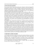
Our model for the heat pump (junction) consists of two quantum systems H and C with
Hamiltonians H
H
and H

C
, respectively; see Fig. 1. Each s ystem has n energy levels and
couples to its thermal bath. Similar models were employed for studying heat engines (18; 19)
and refrigerators (20). It will be seen below that this model admits a classical interpretation,
because all the involved initial and final density matrices will be diagonal in the energy
4
Heat Analysis and Thermodynamic Effects
Enhancing Spontaneous Heat Flow 3
T
c
T
h
Q
h
Q
c
V(t)
W
H
C
Ε
1
Ε
2
Μ
1
Μ
2
Fig. 1. The heat pump model. The few-level systems H and C operate between two baths at
temperatures T

c
and T
h
T
c
< T
h
. During the first step of operation the two systems interact
together either spontaneously or driven by a work-source at the cost of work W.Duringthis
stage couplings with the thermal baths is neglected (thermal isolation). In the second step the
systems H and C do not interact with each other and freely relaxes to their equilibr ium states
(2) under action of the corresponding thermal bath.
representation. We shall however work within the quantum framework, since it is more
intuitive.
Initially, H and C do not interact with each other. Due to coupling with their baths they are in
equilibrium at temperatures T
h
= 1/ β
h
> T
c
= 1/ β
c
[we set k
B
= 1]:
ρ
= e
−β
h

H
H
/tr [e
−β
h
H
H
], σ = e
−β
c
H
C
/tr [e
−β
c
H
C
],(2)
where ρ and σ are the initial Gibbsian density matrices of H and C, respectively. We write
ρ
= diag[r
n
, , r
1
], σ = diag[s
n
, , s
1
],(3)
H

H
= diag[ ε
n
, ,ε
1
= 0 ], H
C
= diag[ μ
n
, ,μ
1
= 0 ],
where diag
[a, , b] is a diagonal matrix with entries (a, , b ), and where without loss of
generality we have nullified the lowest energy level of both H and C. Thus the overall initial
density matrix is
Ω
in
= ρ ⊗ σ,(4)
and the initial Hamiltonian of the junction is
H
0
= H
H
⊗ 1 + 1 ⊗ H
C
.(5)
2.1 Spontaneous regime
During a spontaneous process no work is exchanged with external sources. For our situation
a spontaneous heat transfer will amount to a certain interaction between H and C. Following

to the approach of (25–27) we model this interaction via a Hamiltonian that conserves the
(free) Hamiltonian H
0
[see (5)] for all interaction times. This then realizes the main premise
of spontaneous processes: no work exchange at any time. Our model for spontaneous heat
transfer consists of two steps.
1. During the first step H and C interact with each other [collision]. We assume that this
interaction takes a sufficiently short time δ, and during this time the coupling with the
5
Enhancing Spontaneous Heat Flow
4 Will-be-set-by-IN-TECH
two thermal baths can be neglected [thermal isolation]. The interaction is described by the
Hamiltonian H
int
added to (5):
H
= H
H
⊗ 1 + 1 ⊗ H
C
+ H
int
.(6)
The overall Hamiltonian H again lives in the n
2
-dimensional Hilbert space of the junction
1
.
As argued above, the interaction Hamiltonian commutes with the total Hamiltonian:
[H

0
, H
int
]=0, (7)
making the energy H
0
a conserved quantity
2
. To have a non-trivial effect on the considered
system, the interaction Hamiltonian H
int
should not commute with the separate Hamiltonian:
[H
H
⊗ 1, H
int
] = 0. ForthistobethecasethespectrumofH
0
should contain at least one
degenerate eigenvalue. Otherwise, relations
[H
0
, H
int
]=0and[H
H
⊗ 1, H
0
]=0 will imply
[H

H
⊗ 1, H
int
]=0 (and thus a trivial effect of H
int
), because the eigen-base of H
0
will be
unique (up to re-numbering of its elements and their multiplication by phase factors). The
energy
Q
[sp]
h
= tr

H
H

ρ
− tr
C

e
−
iδ
¯h
H
int
Ω
in

e
iδ
¯h
H
int

,(8)
lost by H during the interaction is gained by C.Heretr
H
and tr
C
are the partial traces.
Commutative interaction Hamiltonians (7) are applied to studying heat transfer in (25–
27). Refs. (25; 26) are devoted to supporting the thermodynamic knowledge via quantum
Hamiltonian models. In contrast, the approach of (27) produced new results.
2. For times larger than δ, H and C do not interact and freely relax back to their equilibrium
states (2, 4) due to interaction with the corresponding thermal baths. These equilibrium states
are reached after some relaxation time τ. Thus the cycle is closed|the junction returns to its
initial state|and Q
[sp]
h
given by (8) is the heat per cycle taken from the hot thermal bath during
the relaxation (and thus during the overall cycle).
It should be obvious that once T
h
> T
c
we get Q
[sp]
h

> 0: heat spontaneously flow from hot to
cold. The proof of this fact is given in (19; 20; 25–27).
For times larger than τ there comes another interaction pulse between H and C,andthecycle
is repeated.
2.1.1 Po wer
Recall that the power of heat-transfer is defined as the ratio of the transferred heat to the cycle
duration τ, Q
[sp]
h
/τ.Forthepresentmodelτ is mainly the duration of the second stage, i.e.,
τ is the relaxation time, which depends on the concrete physics of the system-bath coupling.
For a weak system-bath coupling τ is larger than the internal characteristic time of H and C.
In contrast, for the collisional system-bath interaction, τ can be very short; see Appendix ??.
1
More precisely, we had to write the Hamiltonian (6) as H
H
⊗ 1 + 1 ⊗ H
C
+ α(t)H
int
,whereα(t) is a
switching function that turns to zero both at the initial and final time. This will however not alter the
subsequent discussion in any serious way.
2
This implementation of spontaneous heat-transfer processes admits an obvious generalization: one
need not require the conservation of H
0
for all interaction times, it suffices that no work is consumed
or released within the overall energy budget of the process in the time-interval
[0, δ]. For our purposes

this generalization will not be essential; see (27).
6
Heat Analysis and Thermodynamic Effects
Enhancing Spontaneous Heat Flow 5
Thus the cycle time τ is finite, and the power Q
[sp]
h
/τ does not vanish due to a large cycle
time, though it can vanish due to Q
[sp]
h
→ 0.
Note that some entropy is produced during the free relaxation. This entropy production can
be expressed via quantities introduced in (4–8); see (20) for details. The first step does not
produce entropy, because it is thermally isolated and is realized by a unitary operation that
can be reversed by operating only on observable degrees of freedom (H
+ C). It is seen that
no essential aspect of the considered model depends on details of the system-bath interaction.
This is an advantage.
2.2 Driven regime
The purpose of driving the junction wi th an external field is to enhance [increase] the
spontaneous heat Q
[sp]
h
. The driven regime reduces to the above two steps, but instead of the
spontaneous interaction we have the following situation: the interaction between H and C is
induced by an external work-source. Thus (7) does not hold anymore. The overall interaction
[between H, C and the work-source] is described via a time-dependent potential V
(t) in the
total Hamiltonian

H
H
⊗ 1 + 1 ⊗ H
C
+ V(t) (9)
of H
+ C. The interaction process is still thermally isolated: V(t) is non-zero only in a short
time-window 0
≤ t ≤ δ and is so large there that the influence of the couplings to the baths
can be neglected.
Thus the dynamics of H
+ C is unitary for 0 ≤ t ≤ δ:
Ω
f
≡ Ω (δ)=U Ω
i
U
†
, U = T e
−
i
¯h

δ
0
ds
[
V(s)+ H
0
]

, (10)
where Ω
i
= Ω(0)=ρ ⊗ σ is the initial state defined in (2), Ω
f
is the final density matrix, U is
the unitary evolution operator, and where
T is the time-ordering operator. The work put into
H
+ C reads (1; 3)
W
= E
f
− E
i
= tr[(H
H
⊗ 1 + 1 ⊗ H
C
)(Ω
f
− Ω
i
)], (11)
where E
f
and E
i
are initial and final energies of H + C. Due to the interaction, H (C) looses
(gains) an amount of energy Q

h
( Q
c
)
Q
h
= tr( H
H
[ ρ − tr
C
Ω
f
]), (12)
Q
c
= tr( H
C
[tr
H
Ω
f
− σ ]). (13)
Eqs. (11, 12) imply an obvious relation
W
= Q
c
− Q
h
. (14)
Recall that for spontaneous processes not only the consumed work is zero, W

= 0, but also
the stronger conservation condition (7) holds.
Once H
+ C arrives at the final state Ω
fin
, the inter-system interaction is switched off, and H
and C separately [and freely] relax to the equilibrium states (2). During this process Q
h
is
taken as heat from the hot bath, while Q
c
is given to the cold bath. Note from section 2.1.1 that
the driven operation does not change the cycle time τ, because the latter basically coincides
with the relaxation time. Therefore, increasing Q
h
means increasing heat transfer power.
7
Enhancing Spontaneous Heat Flow
6 Will-be-set-by-IN-TECH
3. Maximization of heat
3.1 Unconstrained maximization
The type of questions asked by thermodynamics concerns limiting, optimal characteristics.
Sometimes the answers are uncovered directly via the basic laws of thermodynamics, an
example being the Carnot bound (1). However, more frequently than not, this goal demands
explicit optimization procedures (9).
We shall maximize the heat Q
h
transferred from the hot bath over the full Hamiltonian of the
junction. For spontaneous processes this amounts to maximizing over Hamiltonian (6) living
in the n

2
-dimensional Hilbert space of the junction H + C and satisfying condition (7). For
driven processes we shall maximize over Hamiltonians (9). In this case we shall impose an
additional condition that the work put into H
+ C in the first step does not exceed E > 0:
W
≤ E. (15)
Once the work put into the system is a resource, it is natural to operate with resources fixed
from above.
Recall that the Hamiltonians (6, 9) live in the n
2
-dimensional Hilbert space. The bath
temperatures T
c
and T
h
and the dimension n
2
(the number of energy levels) will be held fixed
during the maximization.
Due to (8) the maximization of the spontaneous heat Q
[sp]
h
over the Hamiltonians (6, 7)
amounts to maximizing over unitary operators e
iδ
¯h
H
int
, and over the energies {ε

k
}
n
k
=2
, {μ
k
}
n
k
=2
of H and C. Likewise, as seen from (9–11), the maximization of the driven heat Q
h
amounts
to maximizing under condition (15) over all unitary operators
U living in the n
2
-dimensional
Hilbert space, and over the energies
{ε
k
}
n
k
=2
, {μ
k
}
n
k

=2
.
We should stress that the class of Hamiltonians living in the n
2
-dimensional Hilbert space
[with or without constraint (7)] is well-defined due to separating the heat transfer into two
steps (thermally isolated interaction and isothermal relaxation). More general classes of
processes can be envisaged. For instance, we may write the free Hamiltonian as H
0
+ H
B,c
+
H
B,h
,whereH
0
, H
B,c
and H
B,h
are, respectively, the Hamiltonians of the junction and the two
thermal baths. Now the Hamiltonian H
int
of spontaneous processes will be conditioned as
[H
int
, H
0
+ H
B,c

+ H
B,h
]=0. This condition is more general than (7). Then the corresponding
class of driven processes can be naturally defined via the same class of Hamiltonians but
without this commutation condition. We do not consider here such general processes, since
we are not able to optimize them.
As seen below, the maximization of the spontaneously transferred heat (8) amounts to a
particular case of maximizing Q
h
. So we s hall directly proceed to maximizing the driven
heat Q
h
;see(12).
First, take in (15) the simplest case: E
=+∞. This case contains the pattern of the general
solution. Here we have no constraint on maximization of Q
h
and it is done as follows.
Since tr
[H
H
ρ] depends only on {ε
k
}
n
k
=2
, we choose {μ
k
}

n
k
=2
and V(t) so that the final energy
tr
[H
H
tr
C
Ω
f
] attains its minimal value zero. Then we shall maximize tr[H
H
ρ] over {ε
k
}
n
k=2
.
Note from (3)
H
H
⊗ 1 = diag[ ε
1
, , ε
1
, , ε
n
, , ε
n

],
Ω
i
= ρ ⊗ σ = diag[ r
1
s
1
, ,r
1
s
n
, ,r
n
s
1
, ,r
n
s
n
].
It is clear that tr
[
H
H
tr
C
Ω
f
]
=

tr

(H
H
⊗ 1)U Ω
i
U
†

goes to zero when, e.g., s
2
= = s
n
→ 0
(μ
≡ μ
2
= = μ
n
→ ∞), while U amounts to the SWAP operation Uρ ⊗ σU
†
= σ ⊗ ρ.Simple
8
Heat Analysis and Thermodynamic Effects
Enhancing Spontaneous Heat Flow 7
symmetry considerations show that at the maximum of the initial energy tr[H
H
σ] the second
level is n
− 1 fold degenerate, i.e. ε ≡ ε

2
= = ε
n
.Denoting
u
= e
−β
h
ε
∝ r
2
= = r
n
(16)
we obtain for Q
h
= Q
h
(∞)
Q
h
(∞)=T
h
ln

1
u

1
−

1
1 +(n − 1) u

(17)
where u is to be found from maximizing the RHS of (17) over u, i.e., u is determined via
1
+(n − 1)u + ln u = 0. (18)
Note that in this case W
=+∞.Inthen  1 limit we have u =
ln n
n
[
1 + o(1)
]
from (18) and
Q
h
= T
h
ln n

1 + O

ln ln n
ln n

.
3.2 Constrained maximization
ThecaseofafiniteE in (15) is more complicated. We had to resort to numerical recipes
of Mathematica 6. Denoting

{|i
H
}
n
k=1
and {|i
C
}
n
k=1
for the eigenvectors of H
H
and H
C
,
respectively, w e see from (11, 12) that W and Q
h
feel U only via the matrix
C
ij| kl
= |i
H
j
C
|U|k
H
l
C
|
2

. (19)
This matrix is double-stochastic (24):
∑
ij
C
ij| kl
=
∑
kl
C
ij| kl
= 1. (20)
Conversely, for any double-stochastic matrix C
ij| kl
there is some unitary matrix U with matrix
elements U
ij| kl
,sothatC
ij| kl
= |U
ij| kl
|
2
(24). Thus, when maximizing various functions of W
and Q
c
over the unitary U , we can directly maximize over the (n
2
− 1)
2

independent elements
of n
2
× n
2
double stochastic matrix C
ij| kl
. This fact simplifies the problem.
Numerical maximization of Q
h
over all unitaries U|alternatively, over all doubly stochastic C
matrices (19)|and energy spectra
{μ
k
}
n
k=2
and {ε
k
}
n
k=2
constrained by W ≤ E produced the
following results:
• The upper energy levels for both systems H and C are n
− 1 times degenerate [see (3)]:
μ
= μ
2
= = μ

n
, ε = ε
2
= = ε
n
. (21)
• The optimal unitary corresponds to SWAP:
U ρ ⊗ σU
†
= σ ⊗ ρ. (22)
• The work resource is exploited fully, i.e., the maximal Q
h
is reached for W = E.
Though we have numerically checked these results for n
≤ 5 only, we trust that they hold for
an arbitrary n.
Denoting by
Q
h
the maximal value of Q
h
, and introducing from (21)
v
= e
−β
c
μ
and u = e
−β
h

ε
, (23)
9
Enhancing Spontaneous Heat Flow
8 Will-be-set-by-IN-TECH
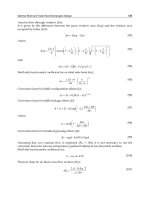
0.0 0.1 0.2 0.3 0.4 0.5
0.1
0.2
0.3
0.4
WT
h
Q
h
T
h
Fig. 2. The optimal transferred heat Q
h
versus work W. Dashed curves refer to
θ
≡ T
c
/T
h
= 0.9: n = 2 (lower dashed curve) and n = 3 (upper dashed curve). Normal
curves refer to θ
= 0.5: n = 2(lowernormalcurve)andn = 3 (upper normal curve).
we have
Q
h

T
h
= ln

1
u

(n − 1)(u − v)
[
1 +(n − 1) v
][
1 +(n − 1) u
]
, (24)
W
T
h
=
(
ln u − θ ln v )(n − 1)(u − v)
[
1 +(n − 1) v
][
1 +(n − 1) u
]
, (25)
where u and v in ( 24, 25) are determined from maximizing the RHS of (24) and satisfying
constraint (25).
An important implication of ( 24, 25) is that
Q

h
(W) is an increasing function of W for all
allowed values of W:
Q
h
(W) > Q
h
(W

) if W > W

. (26)
Fig. 2 illustrates this fact. For fixed parameters T
c
, T
h
and n, the allowed W’s range from a
certain negative value|which corresponds to work-extraction from a two-temperature system
H
+ C|to arbitrary W > 0. Eq. (26) expresses an intuitively expected, but still non-trivial fact
that the best transfer of heat takes place upon consuming most of the available work. Note
that this result holds only for properly optimized values of
Q
h
. One can find non-optimal
set-ups, where (26) is not valid
3
.
3.3 Optimization of spontaneous processes
According to our discussion in section 2.1, the maximization of transferred heat Q

[sp]
h
given
by (8) should proceed over all unitary operators e
−
iδ
¯h
H
int
with H
int
satisfying (7) and over the
energies
{ε
k
}
n
k
=2
, {μ
k
}
n
k
=2
of H and C. This maximization has been carried out along the lines
3
The simplest example is a junction, where the free Hamiltonian H
0
has a non-degenerate energy

spectrum, and thus the condition (7) does not hold. There are no proper spontaneous processes for
this case. Still there can exist a work-exracting (W
< 0) driven processes that transfer heat from hot to
cold.
10
Heat Analysis and Thermodynamic Effects
Enhancing Spontaneous Heat Flow 9
described around (20). We obtained that the maximal spontaneous heat Q
[sp]
h
is equal to Q
h
in (24) under condition W = 0:
Q
[sp]
h
= Q
h
(W = 0). (27)
Thus the optimal spontaneous processes coincide with optimal processes with zero consumed
work. This result is non-trivial, because the class of unitary operators with W
= 0islarger
than the class of unitary operators e
−
iδ
¯h
H
int
with H
int

satisfying (7). Nevertheless, these two
classes produce the same maximal heat.
• Eqs. (26, 27) imply that if the spontaneous heat transfer process is already optimal (with
respect to the junction Hamiltonian) its enhancement with help of driven processes does
demand work-consumption, W
> 0. This fact is non-trivial, because|as well known from
the theory of heat-engines|also work-extraction does lead to the heat flowing from cold to
hot (1; 3).
Taking W
= 0 in (24, 25) and recalling (23) we get
μ
= ε, u = v
θ
. (28)
The interpretation o f (28) is that since there are only two independent energy gaps i n the
system, they have to be precisely matched for the spontaneous processes to be possible; see in
this context the discussion after (7). Thus the spontaneous heat
Q
[sp]
h
is given as
Q
[sp]
h
T
c
= ln

1
v

0

(n − 1)(v
θ
0
− v
0
)
[1 +(n − 1)v
θ
0
][1 +(n − 1)v
0
]
, (29)
where v
0
maximizes the RHS of (29).
3.4 How much one can enhance the spontaneous process?
We would like to compare the optimal spontaneous heat (29) with the optimal heat Q
h
(∞)
transferred under consumption of a large amount of work; see (17, 18) and recall (26). One
notes that for parameters of Fig. 2 the approximate equality
Q
h
(∞) ≈Q
h
(W) is reached
already for W/T

h
< 1. This figure also shows that for the temperature ratio θ ≡ T
c
/T
h
far
from 1, the improvement of the transferred heat introduced by driving is not substantial. It
is however rather sizable for θ
 1, because here the spontaneous heat (29) is close to zero,
while the heat
Q
h
(∞) does not depend on the temperature difference at all; see Fig. 2 and (17,
18).
4. Efficiency
We saw above that enhancing optimal spontaneous processes does require work. Once this is
understood, we can ask how efficient is this work consumption. The efficiency is defined as
χ
(W)=
Q
h
(W) −Q
[sp]
h
W
> 0, (30)
where
Q
h
(W) is the optimal heat transferred under condition that the consumed work is not

larger than W
> 0, while Q
[sp]
h
is the optimal spontaneous heat; see (24, 29). Note that the
11
Enhancing Spontaneous Heat Flow
10 Will-be-set-by-IN-TECH
0.0 0.1 0.2 0.3 0.4 0.5 0.6
0.0
0.2
0.4
0.6
0.8
1.0
W
Χ
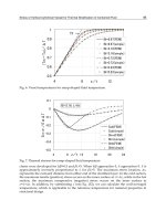
Fig. 3. The efficiency χ versus work W for θ ≡ T
c
/T
h
= 0.5 and n = 2 (normal curve), n = 10
(dashed curve) and n
= 30 (thick curve).
two subtracted quantities
Q
h
(W) and Q
[sp]
h

in (30) refer to the same junction H + C,butwith
different Hamiltonians; see (24, 25).
For W
→ 0, χ(W) increases monotonically and tends to a well defined limit χ(0); see Fig. 3.
•Forfixedθ and n, χ
(0)=χ(W → 0) is the maximal possible efficiency at which the
enhanced heat pump can operate. As s een from Fig. 3, this maximum is reached for
Q
h
(W) −Q
h
(0) → +0andW → +0, (31)
where we recall that n, T
h
and T
c
are held fixed.
• There is thus a complementarity between the driven contribution in the heat, which
according to (26) maximizes for W
→ ∞, and the efficiency that maximizes under W → 0.
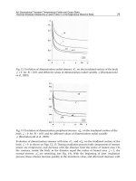
Note from Fig. 4 the following aspect of the maximal efficiency χ
(0): it decreases for a larger
n (and a fixed θ). This is related to the fact that the optimal spontaneous heat
Q
[sp]
h
increases
for larger n.
• It is seen from Fig. 3 that
χ

(W) ≤ χ(0) <
θ
1 − θ
. (32)
We checked that this upper bound for the efficiency (30) holds for all θ
= T
c
/T
h
and n.
It will be seen below that the upper bound
θ
1−θ
is reached in the quasi-equilibrium limit θ → 1.
Note that
θ
1−θ
formally coicides with the Carnot limiting efficiency for ordinary refrigerators;
see (2). A straightforward implication of (32) is that enhancing optimal spontaneous processes
must be inefficient for θ
→ 0.
Let us discuss to which extent the bound (32) is similar to the Carnot bound (2) for
refrigerators.
0. These two expressions are formally identical.
1. Recall that (2) is a general upper bound for the efficiency of refrigerators that transfer
heat against its gradient. Such a transfer does require work-consumption. The same aspect
12
Heat Analysis and Thermodynamic Effects
Enhancing Spontaneous Heat Flow 11
0.0 0.2 0.4 0.6 0.8

0
2
4
6
8
10
Θ
Χ  0
Fig. 4. The maximal efficiency χ(0)=χ(W = 0) given by (??)versusθ = T
c
/T
h
for n = 2
(top normal curve), n
= 101 (bottom normal curve), and n = 10
5
(dotted curve). Thick curve:
the efficiency θ/
(1 − θ).
is present in (30), because by its very construction the efficiency (30) refers to enhancement
of the optimal spontaneous process that also demands work-consumption. To clarify this
point consider a spontaneous process with the transferred heat Q
[sp]
h
. Let this spontaneous
process be n on-optimal in the sense that no full optimization over the Hamiltonians (6, 7)
has been carried out: Q
[sp]
h
< Q

[sp]
h
. This non-optimal process is now enhanced via a
work-consuming one. Denote by Q
h
(W) > Q
[sp]
h
the transferred heat of this process, where
W is the consumed work. Following (30) one can define the efficiency of this enhancement
as χ

(W)=[Q
h
(W) − Q
[sp]
h
]/W. One can now show, see Appendix 8, that χ

(W) can be
arbitrary large for a sufficiently small (but non-zero) consumed work W.Thereasonfor
this unboundness is that we consider a non-optimal spontaneous process, which can be also
enhanced by going to another spontaneous process.
2. We noted above that reaching bound (32) means a neglegible enhancement; see (31).
The same holds for the Carnot bound (2) for refrigerators: operating sharply at the Carnot
efficiency means that the heat transferred during refrigeration is zero; see (20) and references
therein.
3. An obvious point where the bounds (32) and (2) differ from each other is that the latter is a
straightforward implication of the first and second laws of thermodynamics, while the former
is so far obtained in a concrete model only. We opine however that its applicability domain is

larger than this model; some support for this opinion is discussed in section 5.
5. Enhanced heat transfer in linear non-equilibrium thermodynamics
Since the above results were obtained on a concrete model, one can naturally question their
general validity. Here we indicate that these results are recovered from the formalism of linear
non-equilibrium thermodynamics (28–30). This theory deals with two coupled processes:
heat transfer between two thermal baths and work done by an e xternal field. In co ntrast
to the model studied in previous sections, the field is not time-dependent; e.g., it can be
associated with the chemical potential difference (30). The difference and similarity between
13
Enhancing Spontaneous Heat Flow