Heat and Mass Transfer Modeling and Simulation Part 10 pdf

Modeling and Simulation of Chemical System Vaporization at High Temperature:
Application to the Vitrification of Fly Ashes and Radioactive Wastes by Thermal Plasma

171
4. Transfer equation
4.1 Determination of the stoichiometric coefficient
To simplify the writing and calculation of the mass transfer equation at the interface, a
dimensionless quantity X
j
, called stoichiometric coefficient of a metal ‘J’, has been
introduced and corresponding
to :

j
O
j
j
M
n
n

 (13)
where n
O-j
is the mole number of oxygen in the liquid phase related to metal ‘J’, whereas the
term
j
M
n represents the total mole number of metal ‘J’ in the liquid phase, which contains m
species. For example if N is the total mole number of metals in the mixing melted material,
for an unspecified metal ‘J’, the expressions of X

j
is as follows :

1
1
1
m
ij ij
ik i
N
i
i
j
i
j
j
j
m
ij i
i
a
an
a
an










(14)
a
ij
and a
ik
are respectively the stoichiometric coefficients of the element ‘J’, and oxygen in
species ‘i’. n
i
represents the number of moles of species ‘i’.
i
j

is the valence of metal ‘J’ in
oxide ‘i’.
4.2 Example
In an initial mixture of Al-Si-Fe-O-Cl, for example, the species which can exist in the liquid
phase at 1700 K are as follows: SiO
2
, Fe
2
SiO
4
, Fe
3
O
4
, FeO, Al

2
O
3
, AlCl
3
, FeCl
2
. The iron
stoichiometric coefficients X
Fe
in the system is given by the following expression:

24 34
24 34
4
(4 ) 4
8
23
Fe SiO Fe O FeO
Fe
Fe SiO Fe O FeO
nnn
X
nnn
 


(15)
4.3 Transfer equation
From equation (13), the oxygen mole number in the liquid phase related to metal ‘J’, can be

deduced, i.e.

.
j
O
jj
M
nn


 (16)
If equation (16) is differentiated relatively to time and each term is divided by the surface of
the interface value A, it comes
:

11 1
j
j
M
O
jj
jM
dn
dn d
n
A
dt A dt A dt




(17)

Heat and Mass Transfer – Modeling and Simulation

172
The interfacial density of molar flux of a species ‘i’ is:

1
i
i
dn
J
A
dt

(mole.s
-1
.m
-2
) (18)
Introducing equation (18), in equation (17), leads to:

() .( )
J
jj
M
j
LL
OM j M
n

d
JJ
A
dt

 
(19)
()
j
L
OM
J
represent the surfacic molar flux densities of oxygen related to metal ‘J’ from the
liquid phase, whereas
()
j
L
M
J
is the equivalent density of molar flux of a metal J from the
liquid phase.
The total surfacic densities of molar flux of oxygen from the
liquid phase is expressed by:

1
() ()
j
N
LL
OOM

j
JJ



(20)
If in the equation (20)
()
j
L
OM
J
is replaced by its expression given by the equation (19) it
follows:

11
1
() ( ) .
jj
NN
j
LL
OjM M
jj
d
JJn
Adt


 


(21)
Indicating by Ng, the number of species which can exist in the vapor phase, the
expressions of the total densities of molar flux of oxygen and an unspecified metal ‘J’ in gas
phase are
:

1
()
Ng
GG
Oiki
i
JaJ



(22)

1
()
j
Ng
GG
M
i
j
i
i
JaJ




(23)
where J
i
G
is the molar flux density of a gas species ‘i’.
The mass balance at the interfacial liquid to gas is expressed by the equality between the
equivalent densities of molar flux of an element in the two phases, i.e.
:
()()
LG
ii
JJ (24)
The use of matter conservation equations at the interface, for oxygen and metals, and the
combination of equations (16), (17), (18), (19) and (20), lead to the following equation.

111
1
() . 0
jj
Ng
NN
j
GG
jM iki M
jij
dX
XJ aJ n

Adt




(25)
Modeling and Simulation of Chemical System Vaporization at High Temperature:
Application to the Vitrification of Fly Ashes and Radioactive Wastes by Thermal Plasma

173
The equation (25) is the oxygen matter conservation equation or the transfer equation at the
interface. Argon is used as a carrier gas. In the plasma conditions, it is supposed that argon
is an inert gas, so its molar flux density is zero:

0
G
Ar
J

(26)
The density flux for a gas species ‘i’ is given by:

().
xw
Gw
ii i
iTi
i
Dp p
JJ

p
RT


 
(27)
where
w
i
p
and
x
i
p
represent the interfacial partial pressure and the partial pressure in the
carrier gas of species ‘i’ respectively; J
T
is the total mass flux density with
1
11
,0 1
nn
GG w
TiAr i
ii
JJJandpatm


 


, 
i
is boundary layer thickness, and D
i
is diffusion
coefficient.
5. Flux retained by the bath
The Faraday's first law of electrolysis states that the mass of a substance produced at an
electrode during electrolysis is proportional to the mole number of electrons (the quantity of
electricity) transferred at that electrode [10]:

A
QM
m
q
N


(28)
where
m is the mass of the substance produced at the electrode (in grams), Q is the total
electric charge passing through the plasma (in coulombs),
q is the electron charge, v is the
valence number of the substance as an ion (electrons per ion),
M is the molar mass of the
substance (in grams per mole), and
N
A
is Avogadro's number. If the mole number of a
substance

i is initially
0
i
n , its mole number produced at the electrode is:

0
ii
A
Q
nn
qvN

(29)
The interfacial density of molar flux of a species ‘
i’ is:

1
i
i
dn
J
Adt

(mole.s
-1
.m
-2
) (30)
The density (
i

R
J ), of molar flux of a species i retained by the bath under the electrolyses
effects, can be obtained by substituting (29) in (30) to yield:

0
0
11

i
i
A
R
ii
A
Q
dn
qvN
dn n
dQ
J
A
dt A dt A
q
Nvdt



 
(31)

Heat and Mass Transfer – Modeling and Simulation

174
dQ
I
dt

represents the current in the plasma and
1
96485 .
A
F
q
NCmol


is Faraday's
constant. Equation (31) becomes:

0

i
R
i
I
J
n
AFv

(32)

6. Numerical solution
Newton’s numerical method solves the mass balance equations (26), (27) and (28) with
respect to the interfacial thermodynamic equilibrium, the unknown parameters being the
interfacial partial pressure
w
i
P
, the stoichiometric coefficient
J
X and the molar flux densities
G
i
J
.
The convergence scheme is as follows:
-
We calculate the liquid-gas interfacial chemical composition of the closed system by
using Ericksson’s program. The oxygen partial pressure is then defined by the
convergence algorithm.
-
The recently known values of
w
i
p
and
J
X are introduced into the mass equilibrium
equations which can be solved after a series of iterative operations up to the algorithm
convergence.
-

At the beginning of the next vaporization stage, the system is restarted with the new
data of chemical composition. The time increment is not constant and should be
adjusted to the stage in order to prevent convergence instabilities when a sudden local
variation of the mass flux density occurs.
7. Estimation of the diffusion coefficients
Up to temperatures of about 1000 K, the binary diffusion coefficients are known for current
gases, oxygen, argon, nitrogen…etc. For temperatures higher than 1000 K, the diffusion
coefficients of the gas species in the carrier gas are calculated according to level 1 of the
CHAPMAN-ENSKOG approximation [11]:

3
(1.1)*
2*
()/2
0.002628
()
i
j
i
j
ij
ij ij
ij
TM M MM
D
PT





(33)
In this equation D
ij
is the binary diffusion coefficient (in cm
2
.s
-1
) , M
i
and M
j
are the molar
masses of species ‘i’ and ‘j’. P is the total pressure (in atm), T is the temperature (in K),
*
ij
k
TT


is the reduced temperature, K is the Boltzmann constant, 
ij
is the collision
diameter (in Å),

ij
is the binary collision energy and
(1.1)*
*
()
ij

T
is the reduced collision
integral.
For an interaction between two non-polar particles ‘i’ and ‘j’:


i
j
i
j



(34)
Modeling and Simulation of Chemical System Vaporization at High Temperature:
Application to the Vitrification of Fly Ashes and Radioactive Wastes by Thermal Plasma

175


1
2
ij i j



(35)
The values relating to current gases needed for our calculations are those of Hirschfelder
[11]. For the other gas species, such as the metal vapor, the parameters of the intermolecular
potential remain unknown whatever the interaction potential used. This makes impossible

the determination of the reduced collision integral. For this reason the particles are regarded
as rigid spheres and the collision integrals are assimilated to those obtained with the rigid
spheres model [12]. That is equivalent to the assumption:


(1.1)*
*
()
ij
T = 1 (36)

i
j
i
j
rr


 (37)
The terms r
i
and r
j
are the radii of the colliding particles. For the monoatomic particles, the
atomic radii are already found. For the polyatomic particles, the radii of the complex
molecules A
n
B
m
are unknown. Thus it has been supposed that they had a spherical form and

their radii were estimated according to [12]:


1
33
3
nm
AB A B
rnrmr
(38)
In the above expression, r
A
and r
B
are either of the ionic radius, or of the covalence radius
according to the existing binding types. The radii of all the ions which form metal oxides
and chlorides are extracted from the Shannon tables [13].
At high temperature (T > 1000 K), the D
ij
variation law with the temperature is close to the
power 3/2 [14]. For this reason the diffusion coefficients of the gas species are calculated
with only one value of temperature (1700 K). For the other temperatures the following
equation is applied:

3
2
2
21
1
() ().

ij ij
T
DT DT
T




(39)
8. Application of the model
To simulate the same emission spectroscopy conditions in which the experimental
measurement are obtained, the containment matrix used for this study is formed by basalt,
and its composition is given in table 1.
At high temperatures (T > 1700K), in the presence of oxygen and argon, the following
species are preserved in the model:
-
In the vapor phase: O
2
, O, Mg, MgO, K, KO, Na, Na
2
, NaO, Ca, CaO, Si, SiO, SiO
2
, Al,
AlO, AlO
2
, Fe, FeO, Ti, TiO, TiO
2
, and Ar.
- In the condensed phase : CaSiO
3

,Ca
2
SiO
4
, CaMgSi
2
O
6
, K
2
Si
2
O
5
, SiO
2
, Fe
2
SiO
4
, Fe
3
O
4
,
FeO, FeNaO
2
, Al
2
O

3
, CaO, Na
2
O, Na
2
SiO
3
, Na
2
Si
2
O
5
, K
2
O, K
2
SiO
3
, MgO, MgAl
2
O
4
,
MgSiO
3
, Mg
2
SiO
4

, CaTiSiO
5
, MgTi
2
O
5
, Mg
2
TiO
4
, Na
2
Ti
2
O
5
, Na
2
Ti
3
O
7
, TiO, TiO
2
, Ti
2
O
3
,
Ti

3
O
5
, and Ti
4
O
7
.

Heat and Mass Transfer – Modeling and Simulation

176
Elements M
g
K Na Ca Si Al Fe Ti
Chemical form MgO K
2
O Na
2
O CaO SiO
2
Al
2
O
3
FeO TiO
2

% in mass 10.2 1.2 3 8.8 50.4 12.2 11.9 2.2
Cation mole

number

0.253 0.021 0.154 0.157 0.838 0.239 0.165 0.034
Table 1. Composition of basalt
This study focuses on the three radioelements
137
Cs,
60
Co, and
106
Ru. Ruthenium is a high
activity radioelement, and it is an emitter of α, β and γ radiations, with long a radioactive
period. However, Cesium and Cobalt are two low activity radioelements and they are
emitters of β and γ radiations with short-periods on the average (less than or equal to 30
years) [15]. To simplify the system, the radioelements are introduced separately in the
containment matrix, in their most probable chemical form. Table 2 recapitulates the
chemical forms and the mass percentages of the radioelements used in the system.
The mass
percentages chosen in this study are the same as that used in experimental measurements
made by [9, 16].

radioelement
137
Cs
60
Co
106
Ru
Most probable chemical form Cs
2

O CoO Ru
% in mass 10 10 5
Table 2. Chemical Forms and Mass Percentages of radioelement
The addition of these elements to the containment matrix, in the presence of oxygen, leads to
the formation of the following species:
-
In the vapor phase: Cs, Cs
2
, CsK, CsNa, CsO, Cs
2
O, Cs
2
O
2
, Ru, RuO, RuO
2
, RuO
3
, RuO
4
,
Co, Co
2
, and CoO.
-
In the condensed phase: Cs, Cs
2
O, Cs
2
O

2
, Cs
2
SiO
3
, Cs
2
Si
2
O
5
, Cs
2
Si
4
O
9
, Ru, CoAl, CoO,
Co
2
SiO
4
, CoSi, CoSi
2
, Co
2
Si, and Co.
These species are selected with the assistance of the HSC computer code [17]. In the
simulation, the selected formation free enthalpies of species are extracted from the tables of
[18-20].

9. Simulation results
In this part we will present only the results of radioelement volatility obtained by our
computer code during the treatment of radioactive wastes by plasma. However the results
of heavy metal volatility during fly ashes treatment by thermal plasma can be find in [4,5].
9.1 Temperature influence
To have the same emission spectroscopy conditions in which the experimental measurement
are obtained [9, 16], in this study the partial pressure of oxygen in the carrier gas
2
O
P is
fixed at 0.01 atm, the total pressure P at 1 atm, and the plasma current I at 250 A. Figures 2
and 3 depict respectively, the influence of bath surface temperatures on the Cobalt and
Ruthenium volatility. Up to temperatures of about 2000 K, Cobalt is not volatile. Beyond this
Modeling and Simulation of Chemical System Vaporization at High Temperature:
Application to the Vitrification of Fly Ashes and Radioactive Wastes by Thermal Plasma

177
value, any increase of temperature causes a considerable increase in both the vaporization
speed and the vaporized quantity of
60
Co. This behavior was also observed for
137
Cs [8].
Contrarily to Cobalt, Ruthenium has a different behavior with temperature. For
temperatures less than 1700 K and beyond 2000 K, Ruthenium volatility increases whith
temperature increases. Whereas in the temperature interval between 1700 K and 2000 K, any
increase of temperature decreases the
106
Ru volatility.
To better understand this Ru behavior, it is necessary to know its composition at different

temperatures. Table 3 presents the mole numbers of Ru components in the gas phase at
different temperatures obtained from the simulation results.

species Ru RuO RuO
2
RuO
3
RuO
4

Mole
numbers
1700K 6.10
-14
3.10
-10
4.10
-6
7.10
-5
1.10
-6

2000K 5.10
-11
2.10
-8
1.10
-5
3.10

-5
1.10
-7

2500K 1.10
-7
2.10
-6
8.10
-5
1.10
-5
2.10
-8

Table 3. Mole numbers of Ru components in the gas phase at different temperatures

0
0.014
0.028
0.042
0 2000 4000 6000
Time (s)
Mole Number of Co
remainder in the liquid phase
T=2500 K
T=2400 K
T=2200 K
T=1700 K
P

O2
=0.01atm
I=250 A

Fig. 2. Influence of temperature on Co volatility
The first observation that can be made is that the mole numbers of Ru, RuO, and RuO
2

increase with temperature, contrary to RuO
3
and RuO
4
whose mole numbers decrease with
increasing temperatures. These results are logical because the formation free enthalpies of
Ru, RuO, and RuO
2
decrease with temperature. Therefore, these species become more stable
when the temperature increases, while is not the case for RuO
3
and RuO
4
. A more
interesting observation is that at temperatures between 1700 and 2000 K the mole numbers
of Ru, RuO, and RuO
2
increase by an amount smaller that the amount of decrease of the

Heat and Mass Transfer – Modeling and Simulation

178

mole numbers of RuO
3
and RuO
4
resulting in an overall reduction of the total mole numbers
formed in the gas phase. At temperature between 2000 and 2500 K the opposite
phenomenon occurs.

0
0.01
0.02
0.03
0.04
0.05
200 1700 3200 4700 6200
Time (s)
Mole number of Ru
remainder in the liquid phase
T = 2500 K
T = 2000 K
T = 1700 K
P
O2
= 0.01 atm
I = 250
A

Fig. 3. Influence of temperature on Ru volatility
9.2 Effect of the atmosphere
The furnace atmosphere is supposed to be constantly renewed with a composition similar

to that of the carrier gas made up of the mixture argon/oxygen. For this study, the
temperature is fixed at 2500 K, the total pressure P at 1 atm and the plasma current I
at 250 A. Figures 4 and 5 present the results obtained for
60
Co and
106
Ru as a function of
2
O
P .
For
60
Co, a decrease in the vaporization speed and in the volatilized quantity can be noticed
when the quantity of oxygen increases, i.e., when the atmosphere becomes more oxidizing.
The presence of oxygen in the carrier gas
supports the incorporation of Cobalt in the
containment matrix. The same behavior is observed in the case of
137
Cs in accordance with
2
O
P [8].
When studying the Ruthenium volatility presented in the curves of figure 5 it is found that,
contrary to
60
Co, this volatility increases with the increase of the oxygen quantity. This
difference in the Ruthenium behavior compared to Cobalt can be attributed to the redox
character of the majority species in the condensed phase and gas in equilibrium. For
60
Co,

the oxidation degree of the gas species is smaller than or equal to that of the condensed
phase species, hence the presence of oxygen in the carrier gas
supports the volatility of
60
Co.
Whereas
106
Ru, in the liquid phase, has only one form (Ru). Hence, the oxidation degree of
the gas species is greater than or equal to that of liquid phase species and any addition of
oxygen in the gas phase increases its volatility.
Modeling and Simulation of Chemical System Vaporization at High Temperature:
Application to the Vitrification of Fly Ashes and Radioactive Wastes by Thermal Plasma

179
0
0.01
0.02
0.03
0.04
0 1500 3000 4500 600
0
Time(s)
Mole Number of Co
remainder in the liquid phase
P
O2
=0.01 atm
P
O2
=0.1 atm

P
O2
=0.3 atm
P
O2
=0.5 atm

Fig. 4. Influence of the atmosphere nature on the Co volatility

0
0.01
0.02
0.03
0.04
0.05
0 2000 4000 6000 8000
Time (s)
Mole number of Ru
remainder in the liquid phase
P
O2
=0.5 atm
P
O2
=0.3 atm
P
O2
=0.1 atm
P
O2

=0.01 atm
T=2500 K I=250 A

Fig. 5. Influence of the atmosphere nature on the Ru volatility

Heat and Mass Transfer – Modeling and Simulation

180
9.3 Influence of current
To study the influence of the current on the radioelement volatility, the temperature and the
partial pressure of oxygen are fixed, respectively, at 2200 K and at 0.2 atm, whereas the
plasma current is varied from 0 A to 600 A. Figures 6 and 7 depict the influence of plasma

0
0.01
0.02
0.03
0.04
0 2000 4000 6000 8000
Time (s)
Mole Number of Co
remainder in the liquid phase
I = 0 A
I = 300
A
I = 600
A

Fig. 6. Influence of plasma current on Co volatility

0
0.016
0.032
0.048
0.064
0 500 1000 1500 2000 250
0
time (s)
Mole number of Cs
remainder in the liquid phase

Fig. 7. Influence of current on Cs volatility
Modeling and Simulation of Chemical System Vaporization at High Temperature:
Application to the Vitrification of Fly Ashes and Radioactive Wastes by Thermal Plasma

181
current on the Cobalt and Cesium volatility. The curves of these figures indicate that the
increase of the plasma current considerably increases both the vaporization speed and the
vaporized quantity of
60
Co and
137
Cs.
In the model, the electrolyses effects are represented by the ions flux retained by the bath,
given by equation (32), which depends essentially on the plasma current. As the evaporation
kinetics decrease with intensity current, the bath is in cathode polarization which prevents
60
Co and
137
Cs from leaving the liquid phase. Theses results assert the validity of equation

(32) used by this computer code and conforms to the experimental results obtained by
spectroscopy emission [9, 16]. The same behavior is observed in the case of
106
Ru as a
function of plasma current.
9.4 Influence of matrix composition
Three matrices are used in this study and their compositions are given in table 4. Matrix 1 is
obtained by the elimination of 29 g of Silicon for each 100 g of basalt, whereas matrix 2 is
obtained by the addition of 65 g of Silicon for each 100 g of basalt, and matrix 3 is basalt.
Figures 8 and 9 depict the influence of containment matrix composition, respectively, on the
Cobalt and Cesium volatility. The increase of silicon percentage in the containment matrix
supports the incorporation of
60
Co and
137
Cs in the matrix.
For
137
Cs, the increase of silicon percentage in the containment matrix is accompanied by an
increase in mole numbers of Cs
2
Si
2
O
5
and Cs
2
Si
4
O

9
in the condensed phase. The presence of
these two species in addition to Cs
2
SiO
3
in significant amounts (between 10
-3
and 10
-2
mole)
prevents Cs from leaving the liquid phase and reduces its volatility. For Cobalt, the increase of
silicon percentage in the system supports the confinement of
60
Co in the condensed phase in
the Co
2
SiO
4
form. Ruthenium is not considered in this study because, in the liquid phase, it has
only the Ru form and any modification in the containment matrix has no effect on its volatility.

0
0.01
0.02
0.03
0.04
0 1500 3000 4500 6000
Time (s)
Mole Number of Co

remainder in the liquid phase
Matrix 1
Matrix 2
Basalt

Fig. 8. Influence of matrix composition on Co volatility

Heat and Mass Transfer – Modeling and Simulation

182
0
0.018
0.036
0.054
0.072
0 1000 2000 3000
Time(s)
Mole numbers of Cs
remainder I the liquid phase
Matrix 1
Matrix 2
Basalt

Fig. 9. Influence of matrix composition on Cs volatility
9.5 Distribution of Co and Ru on its elements during the treatment
Figures 10 and 11 depict the distribution of Cobalt components on the liquid and gas phases.
In the gas phase, Cobalt exists essentially in the form of Co and, to a smaller degree, in the
CoO form. In the liquid phase, Cobalt is found in quasi totality in CoO, Co and Co
2
SiO

4
forms.
Figure 12 presents the distribution of Ruthenium components on the liquid and gas phases. In
the gas phase, Ruthenium exists essentially in the form of RuO
2
and, to a smaller degree, in the
form of RuO
3
and RuO, whereas Ru and RuO
4
exist in much smaller quantities compared to
the other forms. In the liquid phase, Ruthenium has only the Ru form.

-14
-10.5
-7
-3.5
0
0 1500 3000 4500 6000
Time (s)
Mole number (in log)
Co
2
Si
CoAl
CoSi
Co
2
SiO4
Co

CoO

Fig. 10. Variation of the mole numbers of Co composition in the gas phase
Modeling and Simulation of Chemical System Vaporization at High Temperature:
Application to the Vitrification of Fly Ashes and Radioactive Wastes by Thermal Plasma

183
-14
-10.5
-7
-3.5
0
0 1500 3000 4500 6000
time (s)
Mole number (in log)
Co
2
Si
CoAl
CoSi
Co
2
SiO4
Co
CoO

Fig. 11. Variation of the mole numbers of Co composition in the liquid phase

-9
-7

-5
-3
-1
0 2000 4000 6000 8000
Time (s)
Mole number (in Log)
RuO
2
(g)
RuO
3
(g)
RuO(g)
RuO
4
(g)
Ru(g)
Ru

Fig. 12. Variation of the mole numbers of Ru composition in the gas and liquid phases

Heat and Mass Transfer – Modeling and Simulation

184
10. Comparison with the experimental results
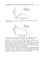
The experimental setup is constituted of a cylindrical furnace, which supports a plasma
device with twin-torch transferred arc system. The two plasma torches have opposite
polarity. The reactor and the torches are cooled with water under pressure by two
completely independent circuits. Argon is introduced at the tungsten cathode and the
copper anode while oxygen, helium and hydrogen are injected through a water-cooled

pipe [21]. To perform spectroscopic diagnostic above the molten surface, a water cooled
stainless-steel crucible is placed under the coupling zone of the twin plasma torches. This
crucible is filled with basalt and 10 % in oxide mass of Cs. On the cooled walls, the
material does not melt and, hence, runs as a self-crucible. The intensities of the Ar line
(λ = 667.72 nm) and the Cs line (λ = 672.32 nm) are measured by using an optical emission
spectroscopy method (figure 13). The molar ratio Cs/Ar is deduced from the intensity
ratio of the two lines [9, 16].





Fig. 13. Schematic of the experimental setup: (1) reactor vessel; (2) cathode torch; (3) anode
torch; (4) spherical-bearing arrangement; (5) injection lance; (6) crucible; (7) porthole; (8)
optical system; (9) monochromator; (10) OMA detector; (11) computer.
Figure 14 shows the code results in comparison with the experimental measurements.
This figure reveals that the experimental and simulation results are relatively close. The
Ar
Ar

O
2
, H
2
,
OES Arrangement
example of spectrum: Cs line (λ = 672.32 nm)

λ

1
23 4 5
6
7
8
9
10
11
Modeling and Simulation of Chemical System Vaporization at High Temperature:
Application to the Vitrification of Fly Ashes and Radioactive Wastes by Thermal Plasma

185
small difference between the simulation results and the experimental measurements can
be attributed to the measurements errors. In fact, the estimated error committed on the
measurement of the ratio Cs/Ar is around 10% [9, 16]. The model calculations assumed a
bath fully melted and homogeneous from the beginning (t = 0s), while in practice
the inside of the crucible is not fully melted and there is a progress of fusion front that
allows a permanent alimentation of the liquid phase in elements from the solid. These
causes explain the perturbation of the experimental measurements and the large gap
between these measurements and the results obtained by the model in the first few
minutes.

0.0E+00
5.0E-05
1.0E-04
1.5E-04
2.0E-04
0 300 600 900
Time (s)
Cs/Ar (molar ratio)

Fig. 14. Comparison between the simulation and experimental results in the case of Cs
11. Conclusion
The objective of this method is to improve the evaporation phenomena related to the
radioelement volatility and to examine their behavior when they are subjected to a heat
treatment such as vitrification by arc plasma. The main results show that up to
temperatures of about 2000 K, Cobalt is not volatile. For temperatures higher than 2000 K,
any increase in molten bath temperature causes an increase in the Cobalt volatility.
Ruthenium, however, has a different behavior with temperature compared to Cobalt. For
temperatures less than 1700 K and beyond 2000 K, Ruthenium volatility increases when
temperature increases. Whereas in the temperature interval from 1700 K to 2000 K, any
increase of temperature decreases the Ru volatility. Oxygen flux in the carrier gas
supports the radioelement incorporations in the containment matrix, except in the case of
the Ruthenium which is more volatile under an oxidizing atmosphere.
For electrolyses

Heat and Mass Transfer – Modeling and Simulation

186
effects, an increase in the plasma current considerably increases both the vaporization
speed and the vaporized quantities of Cs and Co. The increase of silicon percentage in the
containment matrix supports the incorporation of Co and Cs in the matrix. The
comparison between the simulation results and the experimental measurements reveals
the adequacy of the computer code.
12. Acknowledgements
This work was supported by the National Plan, for Sciences, Technology and innovation, at
Al Imam Muhammed Ibn Saud University, college of Sciences, Kingdom of Saudi Arabia.
13. Nomenclature
D
i

J : diffusion flux density for the gas species i.
R
i
J : flux retained by the bath for the gas species i.
G: free energy of a system
g
i
0
: formation free enthalpy of a species under standard conditions,
R : perfect gas constant,
T : temperature,
n
i
: mole number of species i.
p
i
: partial pressure of a gas species
X
i
: molar fraction of species i in the liquid phase.
P : total pressure,
g
n

: total mole number of the species in the gas phase,
l
n

: total mole number of the species in the condensed phase
a

ij
: atoms grams number of the element j in the chemical species i
B
j
: total number of atoms grams of the element j in the system.
n
O2
: equivalent mole number of oxygen
L: Lagrange function
j

: Lagrange multipliers
ξ (n
i
) : Taylor series expansion of F (F=G/RT)
n
O-j
: mole number of oxygen in the liquid phase related to metal ‘J’
j
M
n : total mole number of metal ‘J’ in the liquid phase
i
j

: valence of metal ‘J’ in oxide ‘i’
A: value of interface surface
i
J : interfacial density of molar flux of a species ‘i’

i

: boundary layer thickness
D
i
: diffusion coefficient
m : mass of the substance produced at the electrode
Q : total electric charge passing through the plasma
q : electron charge
v : valence number of the substance as an ion (electrons per ion)
Modeling and Simulation of Chemical System Vaporization at High Temperature:
Application to the Vitrification of Fly Ashes and Radioactive Wastes by Thermal Plasma

187
M : molar mass of the substance
N
A
: Avogadro's number
I: current in the plasma
F: Faraday's constant
*
i
j
k
TT

 : reduced temperature
K : Boltzmann constant


ij
: collision diameter


ij
: binary collision energy
(1.1)*
*
()
ij
T : reduced collision integral
r
i
: radius of a particle
14. References
[1] Eriksson G., Rosen E., J. Chemica Scripta, 4:193, (1973)
[2] Pichelin G., Rouanet A., J. Chemical Engineering Science, 46:1635, (1991)
[3] Badie J. M., Chen X., Flamant G., J. Chemical Engineering Science, 52:4381, (1997)
[4] Ghiloufi I., Baronnet J. M., J. High Temperature Materials Process, volume 10, Issue 1, p.
117-139, (2006)
[5] Ghiloufi I., J. High Temperature Materials Process, volume12, Issue1, p.1-10, (2008)
[6] Ghiloufi, I., J. Hazard. Mater. 163, 136-142, (2009)
[7] Ghiloufi, I., J. Plasma Chemistry and Plasma Processing, Volume 29, Number 4 321-331,
(2009)
[8] Ghiloufi I., Amouroux J., J. High Temperature Materials Process, volume 14, Issue 1, p. 71-
84, (2010)
[9] Ghiloufi I., Girold C., J. Plasma Chemistry and Plasma Processing, 31:109–125, (2011)
[10] Serway, Moses, and Moyer, Modern Physics, third edition (2005)
[11] Hirschfelder, J. O., Curtis, C. F., and Bird, R. B., (1954), Molecular Theory of Gases and
Liquids, John Willey & Sons, New-York.
[12] Razafinimanana, M., (1982), "Etude des coefficients de transport dans les mélanges
hexafluorure de soufre azote application à l’arc électrique", Thèse, Université de
Toulouse.

[13] Shannon R. D., Prewitt C. T., (1969), "Effective Ionic Radii Oxides and Fluorides", Acta
Cryst., Vol. B25, pp. 925-946.
[14] Bird R. B., Stewart W. E., Lightfood E. N., (1960): "Transport phenomena" Ed. Willy.
[15] M. Jorda, E. Revertegat, Les clefs du CEA, n◦30, 1995, pp. 48–61.
[16] C. Girold, Incinération/vitrification de déchets radioactifs et combustion de gaz de
pyrolyse en plasma d’arc, Ph.D. Thesis, Université de Limoges, France, 1997.
[17] Outokumpu HSC Chemistry, Chemical Reaction and Equilibrium Modules with
Extensive Thermochemical Database, Version 6, (2006)
[18] Barin I., Thermochemical Data of Pure Substances, Weinheim; Basel, Switzerland;
Cambridge; New York: VCH, (1989)

Heat and Mass Transfer – Modeling and Simulation

188
[19] Chase Malcolm, NIST-JANAF, Thermochemical Tables, Fourth Edition, J. of Phys. and
Chem. Ref. Data, Monograph No. 9, (1998)
[20] Landolt-Bornstein, Thermodynamic Properties of Inorganic Material, Scientific Group
Thermodata Europe (SGTE), Springer-Verlag, Berlin-Heidelberg, (1999)
[21] S.
Megy, S. Bousrih, J.M.,Baronnet, E.A. Ershov-Pavlov, J.K. Williams, D.M. Iddles, J.
Plasma Chemistry and Plasma Processing, 15, n° 2, (1995), 309 - 319.
9
Nonequilibrium Fluctuations in
Micro-MHD Effects on Electrodeposition
Ryoichi Aogaki
1
and Ryoichi Morimoto
2

1

Polytechnic University, Ryogoku, Sumida-ku, Tokyo,
2
Saitama Prefectural Okubo Water Filtration Plant
Shuku, Sakura-ku, Saitama-shi, Saitama,
Japan
1. Introduction
In copper electrodeposition under a magnetic field parallel to electrode, it is well known
that though the drastic enhancement of deposition rate, a deposit surface receives specific
levelling. This is because the Lorentz force generated by the interaction between magnetic
field and electrolytic current induces a solution flow called magnetohydrodynamic (MHD)
flow with micro-vortex called micro-MHD flow (Figs. 1 and 5a). The former is a laminar
main flow, promoting mass transfer process (MHD effect), and the latter emerges inside the
boundary layer, which often interacts with nonequilibrium fluctuations controlling
electrochemical reactions.
MHD effect is exhibited by the following MHD current equation, where the promotion of
mass transfer by the laminar flow is expressed by the increase of the average current density
z
J (Aogaki et al., 1975).

*1/3*4/3
0z
JHB


 (1)
where ‘< >’ denotes the average with regard to electrode surface, H
*
is a constant, B
0
is the

magnetic flux density, and
*


is the concentration difference between the bulk and surface.
As one of the characteristic results of the electrodeposition in a parallel magnetic field, the
interaction of the micro-MHD flow with nonequilibrium fluctuations called symmetrical
fluctuations suppresses the three-dimensional (3D) nuclei with the order of 0.1 μm in
diameter to yield a flat surface (1st micro-MHD effect) (Aogaki, 2001; Morimoto et al., 2004).
However, after long-term deposition in the same magnetic field, instead of leveling, semi-
spherical secondary nodules with the order of 100 μm in diameters are self-organized from
two-dimensional (2D) nuclei together with the other nonequilibrium fluctuations, i.e.,
asymmetrical fluctuations (2nd micro-MHD effect) (Aogaki et al., 2008a, 2009a, 2010).
On the other hand, in a magnetic field vertical to electrode surface, minute vortexes vertical
to the electrode surface emerge under a macroscopic tornado-like rotation called vertical
MHD flow (Fig. 2); the formers come from 2D nucleation, whereas the latter is generated by
the distortion of current lines in front of a disk electrode. As a result, a characteristic deposit
with regular holes with about 100 μm diameter called micro-mystery circles appears.

Heat and Mass Transfer – Modeling and Simulation

190
Recently, using an electrode fabricated by the electrodeposition in a vertical magnetic field,
the appearance of chirality in enantiomorphic electrochemical reactions was found, and it
was suggested that the selectivity of the reactions comes from the chirality of the vortexes
formed on the electrode (Mogi & Watanabe, 2005; Mogi, 2008).


B
i

f
f
f
d
e
d
e
x
1
0
x
2

x
a
b
c
X
Y
Z

Fig. 1. MHD main flow and boundary layer. a, Luggin capillary; b, working electrode; c,
counter electrode; d, diffusion layer; e, hydrodynamic boundary layer; f, streamline (Aogaki
et al., 1975).


Fig. 2. Vertical MHD flow. 1, electrode; 2, electrode sheath; I, upward spiral flow; II,
rotating flow; B, magnetic field (Sugiyama et al., 2004).
All these phenomena are attributed to the evolution or suppression process of nucleus by
nonequilibrium fluctuations in a magnetic field. Generally, nucleation is classified into two

types; one is 2D nucleation, i.e, expanding lateral growth, and the other is 3D nucleation, i.e.,
protruding vertical growth. These two types of nucleation result from different
nonequilibrium fluctuations. Figure 3 shows two kinds of nonequilibrium fluctuations; one
is asymmetrical fluctuation, which arises from electrochemical reactions in an electrical
double layer. As shown in this figure, this fluctuation one-sidedly changes from an
electrostatic equilibrium state toward cathodic reaction side, controlling 2D nucleation. The
other is symmetrical fluctuation changing around an average value of its physical quantity
in a diffusion layer. This fluctuation controls 3D nucleation. These concentration
fluctuations are defined by