Heat Transfer Engineering Applications Part 13 pot

Air Cooling Module Applications to Consumer-Electronic Products

349
The heat pipe uses the working fluid with much latent heat and transfers the massive heat
from the heat source under minimum temperature difference. Because the heat pipe has
certain characteristics, it has more potential than the heat conduction device of a single-
solid-phase. Firstly, due to the latent heat of the working fluid, it has a higher heat capacity
and uniform temperature inside. Secondly, the evaporation section and the condensation
section belong to the independent individual component. Thirdly, the thermal response time
of the two-phase-flow current system is faster than the heat transfer of the solid. Fourthly, it
does not have any moving components, so it is a quiet, reliable and long-lasting operating
device. Finally, it has characteristics of smaller volume, lighter weight, and higher usability.
Although the heat pipe has good thermal performance for lowering the temperature of the
heat source, its operating limitation is the key design issue called the critical heat flux or the
greatest heat capacity quantity. Generally speaking, we should use the heat pipe under this
limit of the heat capacity curve.
There are four operating limits which are described as following. Firstly, the capillary limit,
which is also called the water power limit, is used in the heat pipe of the low temperature
operation. Specific wick structure which provides for working fluid in circulation is limiting.
It can provide the greatest capillary pressure. Secondly, the sonic limit is that the speed of
the vapour flow increases when the heat source quantity of heat becomes larger. At the
same time, the flow achieves the maximum steam speed at the interface of the evaporation
and adiabatic sections. This phenomenon is similar to the flux of the constant mass flow rate
at conditions of shrinking and expanding in the nozzle neck. Therefore, the speed of flow in
this area is unable to arrive above the speed of sound. This area is known for flow choking
phenomena to occur. If the heat pipe operates at the limited speed of sound, it will cause the
remarkable axial temperature to drop, decreasing the thermal performance of the heat pipe.
Thirdly, the boiling limit often exists for the traditional metal, wick structured heat pipe. If
the flow rate increases in the evaporation section, the working fluid between the wick and
the wall contact surface will achieve the saturated temperature of the vapor to produce

boiling bubbles. This kind of wick structure will hinder the vapour bubbles to leave and
have the vapor layer of the film encapsulated. It causes large, thermal resistance resulting in
the high temperatures of the heat pipe. Fourthly, the entrainment limit is that when the heat
is increased and the vapor’s speed of flow is higher than the threshold value, forcing it to
bear the shearing stress in the liquid; vapor interface being larger than the surface tension of
the liquid in the wick structure. This phenomenon will lead to the entrainment of the liquid,
affecting the flow back to the evaporation section. Besides the above four limits, the choice
of heat pipe is also an important consideration. Usually the work environment can have
high temperature or low temperature conditions which will require a high temperature heat
pipe or a low temperature heat pipe, accordingly. After deciding the operating environment,
the material, internal sintered body, and type of working fluid for the heat pipe are
determined. In order to prevent the heat pipe`s expiration, the consideration of the selection
is very important.
3.2 Thermosyphon
This paragraph experimentally investigates a two-phase closed-loop thermosyphon vapor-
chamber system for electronic cooling. A thermal resistance net work is developed in order
to study the effects of heating power, fill ratio of working fluid, and evaporator surface
structure on the thermal performance of the system. This study explored the relationship

Heat Transfer – Engineering Applications

350
between the vapor pressure and water level inside a two-phase closed-loop thermosyphon
thermal module to acquire a theoretical model of the water level height difference of the
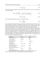
thermal module through the analysis of basic condensing and boiling theory. Figure 2
shows the internal vapor pressure and water level through the heat source with the heating
power Q, based on the entire experimental system. The internal vapour pressure and water
level through the heat source with the heating power Q based on the entire experimental
system. The entire physical system can be divided into four control volumes to resolve the
vapour pressure and the friction loss of steam from the first control volume (C.V.1) to the

third control volume (C.V.3), as revealed by formula (7). Furthermore, the liquid static
pressure balance of the fourth control volume (C.V.4) is exhibited by formula (8). The range
of C.V.1 is from the vapor chamber, including the area from the connecting pipe to the
entrance of the condenser region, which encompasses the loss of steam pressure through the
connecting pipe of the insulation materials. The range of C.V.2 is from the entrance to the
outlet of the condenser, which involves a loss of steam pressure after the condenser. The
scope of C.V.3 is from the outlet of the condenser to the connection surface of the vapor
chamber, which entails a loss of steam pressure through the connecting pipe. The scope of
C.V.4 is from the connection surface of the vapor chamber to the same high level in the
connecting pipe of the vapor chamber.


(a) Initial Condition (b) Steady State
Fig. 2. Relationship between vapour pressure and water level

,,1 ,Vi Vi
f
i
PP P



(7)
Where P
V,i
is the vapor pressure of the ith control volume in this system, P
V,i+1
is the vapor
pressure for the steam into (i+1)
th

control volume through i
th
control volume of the
connecting pipe and ΔP
f,i
is the friction loss of the pressure of steam flow.

,4 ,4lVw
PP H



(8)
where P
l,4
is the hydrostatic pressure of the C.V.4 of liquid, γ
w
is the specific weight of
liquid, ΔH is the height difference of the water level between the internal water level of the
vapor chamber and the connecting pipe connected to the condenser.
The equations represented by C.V.1 to C.V.3 are all added up, and P
l, 4
is equal to P
V, 4
and
substituting it into equation (8), ΔH can be obtained as shown in equation (9).

Air Cooling Module Applications to Consumer-Electronic Products

351

3
,
1
1
f
i
w
i
HP



  




(9)
From the equation (9), if there is no pressure drop loss for ΔP
f,1
and ΔP
f,3
of the pipeline and
ΔP
f,2
of the condenser, then the water level inside the vapour chamber and that connected to
the condensation inside condenser will be the same. That is, ΔH is equal to zero.

Fig. 3. Schematic diagram of the calculation of pressure drop loss (a) Pressure drop loss of
the connecting pipe of C.V.1 (b) Pressure drop loss of the connecting pipe of C.V.3 (c)
Pressure drop loss of the condenser
Figure 3(a) and 3(b) show the estimated method for ΔP
f,1
and ΔP
f,3
of the connecting pipe.
According to a previous study, this can be calculated by formula (10).

2
,,,
1
2
i
f
i i vi vi
i
L
P
f
V
D


(10)
Where f
i
is the friction coefficient generated by the steam flow through the pipes, L
i

represents the equivalent length of the connecting pipe, D
i
is the diameter of the connecting
pipe and ρ
v,i
and V
v,i
represent the vapour density and speed respectively.
According to figure 3(c) and previous studies, the method for calculating ΔP
f,2
considers the
shear stress or the friction force at the gas-liquid interface with small control volume.
Formula (11) can be attained based on momentum conservation.

()
wiw
dP dV
y
dZ
g
dZ dZ
dz dy
 



 






(11)
Where δ is the film thickness of the liquid inside the condenser tube, ρ
w
is the liquid density,
μ
w
is the dynamic viscosity of the liquid, τ
i
is the shear stress at the gas-liquid interface,


dP dz is the pressure drop loss generated by the steam flow through the gas-liquid
interface at the condenser, which can be expressed as equation (12).




4
2
vv ww
i
v
dmV mV
dP
g
dz D dz








 










(12)
In which,
v
m

and
w
m

represent the mass flow rate of the steam and liquid, respectively. V
v

and V

w
denote the speed of vapour and liquid. τ
i
is the shear stress of the gas-liquid
interface, as shown in equation (13) below.

Heat Transfer – Engineering Applications

352

22
300
0.005 1
2(14)
i
v
Gx
D
D


















(13)


vv ww
dmV mV
dz






is the pressure drop produced by the mass flow rate of the gas-liquid
interface, which can be expressed as in equation (14).




2
2
2
1
1
vv ww

vw
dmV mV
x
dx
G
dz dz
  









 












(14)

Where G is the mass flow rate flux, x is the mass flow rate fraction and α is the ratio of the
gas channel. Substituting equation (14) into equation (12), the integral of the range from zero
to Z can be obtained by formula (15) as follows.




2
2
*2
00
1
4
()
21
ZZ
i
VV v
vw
x
dx
P P gZ dz G dz
Ddz













   













(15)
Substituting
2
v
A
D
AD








into the above equation, we can obtain the formula (16)
after integration as follows.




2
2
*2
,2
0
1
4
()
22 2
Z
i
fvv v
vw
x
x
PPPGD dzgZ
DD


  








   












(16)
To calculate the right side of the integral term
0
4
2
Z
i
dz
D








of the above formula (16), first,
assume that the internal film growth equation of the liquid is linear. Therefore, the assumed
slope of SP can attain formula (17) as follows.
δ=SP*Z

(17)
And let

D




(18)
Substituting equations (17) and (18) into equation (14), we can obtain formula (19) as
follows.

22
1 300
0.0001
214
i
v
Gx








 







(19)

Air Cooling Module Applications to Consumer-Electronic Products

353
Substituting equation (19) into the right side of the integral term
0
4
2
Z
i
dz
D








of equation
(16), we can obtain formula (20) as follows.

22
0
24
4
0.005
151 ln(1 ) 76 ln(1 )
2
Z
i
v
S
p
ZS
p
Z
Gx
dz
DSp D D



 


















(20)
Finally, by substituting equation (20) back into formula (16), we can obtain ΔP
f,2
with
formula (21) as shown below.




2
2
2
,2
22

1
22
24
0.005
151 ln(1 ) 76 ln(1 )
fcv v
vw
v
x
x
PGD gZ
D
Sp Z Sp Z
Gx
Sp D D

 







   










 



 









(21)
The film thickness δ can be calculated by the formula (22) as follows.

2
3
4
4
() 3()
w
i
wwv fg wv
Zq

gh g



 

 




 

(22)
In which

3
1
8
pw
fg fg
fg w
C
q
hh
hk










 










(23)
Where h
fg
is the latent heat of the working fluid, C
pw
is the constant pressure of the specific
volume of the liquid;
q


is the input heat flux of the heat source and k
w
is the thermal
conductivity of the liquid.

We use Microsoft
®
Visual Basic
TM
6.0 to write the computing interface resulting from the
above empirical formula and calculated the thermal performance and the water level deficit
inside the thermal module of the two-phase closed-loop thermosyphon. The programming
flow chart is shown in Figure 4(a) and the final operation interface is shown in Figure 4(b).
This study discusses the thermal performance of the two-phase closed-loop thermosyphon
thermal module, and indirectly confirms that the working fluid reflows into the condenser
by measuring the wall temperatures of the condenser, which results in the water level
difference phenomenon within the system. Figure 5 shows the theoretical curve of the water
level height difference for the entire closed thermal module system. The solid black line in
the figure is the theoretical water level height difference based on the heat transfer theory of
pool nucleate boiling and film condensation in this study. Comparing the two curves, we
can accurately predict the same level with the height difference between the experimental
curve before the heating power is less than 60W; however, beyond 60W, the water level
height difference obtained in the experimental curve has tended to be horizontal, while the
theoretical curve will increases with the heating power, the water level height difference
increases only slightly.

Heat Transfer – Engineering Applications

354

(a) Programming flow chart (b) Operator interface
Fig. 4. Programming and the operator interface

Fig. 5. The theoretical value of water level difference of vertical type
For the two-phase closed-loop thermosyphon cooling system, the micro-scale water level
difference phenomenon resulting from the condensing and boiling vapor pressure
difference between the evaporator and condenser sections based on the theories of pool
nucleate boiling and film condensation and the validation of experimental method to
measure the wall temperature of condenser. The height of the condenser of the two-phase
closed-loop thermosyphon system can be shortened by 3.14cm by using the theoretical
water level difference model. The working fluid within the two-phase closed-loop

Air Cooling Module Applications to Consumer-Electronic Products

355
thermosyphon system has different heights resulting from the vapor pressure difference
between the evaporator and the condenser sections. This should be noted in the design of
such two-phase heat transfer components. Finally, this study has established a theoretical
height difference model for two-phase closed-loop cooling modules. This can serve as a
reference for future researchers.
3.3 Vapor chamber
This study derives a novel formula for effective thermal conductivity of a vapor chamber
using dimensional analysis in combination with a thermal-performance experimental
method. The experiment selected water as the working fluid filling up in the interior of
vapour chamber. The advantages of water are embodied in its thermal-physics properties
such as extremely high latent heat and thermal conductivity and low viscosity, as well as its
non-toxicity and incombustibility. The overall operating principle of the experiment is
defined as follows: at the very beginning, the interior of the vapour chamber is in vacuum,
after the wall face of the cavity absorbs the heat from its source, the working fluid in the
interior will be rapidly transformed into vapour under the evaporating or boiling
mechanism and fill up the whole interior of the cavity. The resultant vapour will be
condensed into liquid by the cooling action resulted from the convection between the fins
and fan on the outer wall of the cavity, and condensate will reflow to the wall at the heat

source along the capillary structure as shown in figure 6.


Fig. 6. Drawing of the vapor chamber
It discusses these values of one, two and three-dimensional effective thermal conductivity
and compares them with that of metallic heat spreaders. Equation (24) indicates the effective
thermal conductivity k
index
of the vapor chamber, which is the result of the input heat flux
in
q

multiplied thickness (t) of the vapour chamber divided by the temperature difference
∆T
index
. The one-dimensional thermal conductivity (k
z
) is when the index is equal to z and
the temperature difference ∆T
z
equals the central temperature (T
dc
) on the lower surface
minus that (T
uc
) on the upper surface. The two-dimensional thermal conductivity (k
xyd
) is
when the index is equal to xyd and the temperature difference ∆T
xyd

equals the central
temperature (T
dc
) on the lower surface minus mean surface temperature (T
da
). The two-
dimensional thermal conductivity (k
xyu
) is when the index is equal to xyu and the
temperature difference ∆T
xyu
equals the central temperature (T
uc
) on the upper surface
minus mean surface temperature (T
ua
). The three-dimensional thermal conductivity (k
xyz
) is
when the index is equal to xyz and the temperature difference ∆T
xyz
equals mean surface
temperature (T
da
) on the lower surface minus that (T
ua
) on the upper surface.

Heat Transfer – Engineering Applications

356

index
k
in
index
qt
T






(24)
One of major purposes of this study is to deduce the thermal performance empirical formula
of the vapour chamber, and find out several dimensionless groups for multiple correlated
variables based on the systematic dimensional analysis of the [F.L.T.θ.] in Buckingham Π
Theorem, as well as the relationship between dimensionless groups and the effective
thermal conductivity. Figure 6 is the abbreviated drawing of related variables of the vapour
chamber to be confirmed in this article, and the equation (25) is the functional expression
deduced based on related variables in Figure 6. The symbol k
eff
in the equation is the value
of effective thermal conductivity of the vapour chamber, the k
b
is the thermal conductivity
of the material made of the vapour chamber, the symbol k
w
is the value of effective thermal

conductivity of the wick structure of the vapour chamber, the unit of these thermal
conductivities are W/m°C. The symbol h
fg
is latent heat of working fluid which has unit of
J/K. The P
sat
is saturated vapour pressure of working fluid with unit of N/m
2
. The t is the
thickness of vapour chamber. Their unit is m. The symbol A is the area of vapour chamber
and its unit is m
2
.



,,, , ,,,
eff b w in fg sat
KFunctionkk
q
hPtAh




(25)
It can be inferred from equation (25) that there are nine related variables (symbol m
equalling to 9), and the following equation (26) can be inferred by making use of [F.L.T.θ.]
system (symbol r equalling to 4) to do a dimensional analysis of various parameters in the
above-mentioned equation and combining the analysis result with the equation (25).

0.5 2
eff
in
w
bb
sat fg
k
q
k
Ah
kk t
Ph t










 

   


 




 




(26)
The ,β,γ,λ,τ in the equation (26) indicate the constants determined based on the
experimental parameters. We can know from the said equation (26) that effective thermal
conductivity of the vapour chamber is related to controlling parameters of the experiment,
fill-up number of the working fluid influencing h, volume of the cavity influencing t, input
power and area of the heat source influencing q
in
, area of the vapour chamber influencing A.
Thus, this study is designed to firstly use thermal-performance experiment to determine the
thermal performance and related experimental controlling parameters of the vapour
chamber-based thermal, and sort them into the database of these experimental data, then
combine with equation (26) to obtain the constants of the symbols ,β,γ,λ,τ. Let the constant
 be 1. And these constants β,γ,λ,τ are equivalent to 0.13, 0.28, 0.15, and -0.54 based on some
specified conditions in this research, respectively. This window program VCTM V1.0 was
coded with Microsoft Visual Basic
TM
6.0 according to the empirical formula and calculated
the thermal performance of a vapor chamber-based thermal module in this study. These
parameters affect its thermal performance including the dimensions, thermal performance
and position of the vapor chamber. Thus it is very important for the optimum parameters to
be selected to receive the best thermal performance of the vapor chamber-based thermal
module. The program contains two main windows. The first is the selection window

Air Cooling Module Applications to Consumer-Electronic Products

357
adjusted in the program as the main menu as shown in Fig. 7. In this window, the type of
the air direction can be chosen separately. The second window has five main sub-windows.
There are four sub-windows of the input parameters for the thermal module as shown in
Fig. 7. The first sub-window is the simple parameters of the vapor chamber including
dimensions and thermal performance. Fig. 7 shows the second sub-window involving detail
dimensions of a heat sink. The third and fourth sub-windows are the simple parameters
containing input power of heat source, soldering material, and materials of thermal grease
and performance curve of fan. All the input parameters required for this study of the
window program were given and the window program starts. Later, the program examines
the situation by pressing calculated icon. The fifth sub-window is the window showing the
simulation results. In this sub-window, when it is pressed at calculate icon for making
analysis of the thermal performance of a vapor chamber-based thermal module, we can see
a figure as it is shown in Fig. 7.


Fig. 7. Window program VCTM V1.0
Results show that the two and three-dimensional effective thermal conductivities of vapor
chamber are more than two times higher than that of the copper and aluminum heat
spreaders, proving that it can effectively reduce the temperature of heat sources. The
maximum heat flux of the vapor chamber is over 800,000 W/m
2
, and its effective thermal
conductivity will increase with input power increases. It is deduced from the novel formula
that the maximum effective thermal conductivity is above 800W/m°C. Certain error
necessarily exist between the data measured during experiment, value deriving from
experimental data and actual values due to artificial operation and limitation of accuracy of
experimental apparatus. For this reason, it is necessary take account of experimental error to

create confidence of experiments before analyzing experimental results. The concept of
propagation of error is introduced to calculate experimental error and fundamental
functional relations for propagation of error. During the experiment, various items of
thermal resistances and thermal conductivities are utilized to analyze the heat transfer
characteristics of various parts of thermal modules. The thermal resistance and thermal
conductivity belong to derived variable and includes temperature and heating power,
which are measured with experimental instruments. The error of experimental instruments
is propagated to the result value during deduction and thus become the error of thermal
resistance and thermal conductivity values. An experimental error is represented with a

Heat Transfer – Engineering Applications

358
relative error and the maximum relative errors of thermal conductivities defined are within
±5% of k
index
. This study answered how to evaluate the thermal-performance of the vapor
chamber-based thermal module, which has existed in the thermal-module industry for a
year or so. Thermal-performance of the thermal module with the vapor chamber can be
determined within several seconds by using the final formula deduced in this study. One-
and two-dimensional thermal conductivities of the vapor chamber are about 100 W/m°C,
less than that of most single solid-phase metals. Three-dimensional thermal conductivity of
the vapor chamber is up to 910 W/m°C, many times than that of pure copper base plate.
The effective thermal conductivities of the vapor chamber are closely relate to its dimensions
and heat-source flux, in the case of small-area vapor chamber and small heat-source flux, the
effective thermal conductivity are less than that of pure copper material.
4. Air-cooling thermal module in other industrial areas
Air-cooling thermal module in other industrial areas as large-scale motor and LEDs lighting
lamp are discussed in the following paragraphs. And a vapour chamber for rapid-uniform
heating and cooling cycle was used in an injection molding process system especially in

inset mold products.
4.1 Injection mold
There are many reasons for welding lines in plastic injection molded parts. During the
filling step of the injection molding process, the plastic melt drives the air out of the mold
cavity through the vent. If the air is not completely exhausted before the plastic melt
fronts meet, then a V-notch will form between the plastic and the mold wall. These
common defects are often found on the exterior surfaces of welding lines. Not only are
they appearance defects, but they also decrease the mechanical strength of the parts. The
locations of the welding lines are usually determined by the part shapes and the gate
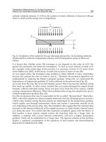
locations. In this paragraph, a heating and cooling system using a vapour chamber was
developed. The vapor chamber was installed between the mold cavity and the heating
block as shown in Fig. 8. Two electrical heating tubes are provided. A P20 mold steel
block and a thermocouple are embedded to measure the temperature of the heat insert
device. The mold temperature was raised above the glass transition temperature of the
plastic prior to the filling stage. Cooling of the mold was then initiated at the beginning of
the packing stage. The entire heating and cooling device was incorporated within the
mold. The capacity and size of the heating and cooling system can be changed to
accommodate a variety of mold shapes.
According to the experimental results, after the completion of molding, 10% of Type1
samples did not pass torque test, while all Type2 and Type3 samples passed the test. After
thermal cycling test, the residual stress of the plastics began to be released due to
temperature change, so the strength of product at the position of weld line was reduced
substantially. Only 30% of Type1 products passed the 15.82 N-m torque tests after thermal
cycling test, followed by 50% of Type2 products and 100% of Type3 products. This study
proved that, among existing insert molding process, the temperature of inserts has impact
on the final assembly strength of product. In this study, the local heating mechanism of
vapor chamber can control the molding temperature of inserts; and the assembly strength
can be improved significantly if the temperature of inserts prior to filling can be increased

Air Cooling Module Applications to Consumer-Electronic Products

359
over the mold temperature, thus allowing the local heating mechanism to improve the weld
line in the insert molding process. In this study, a vapour chamber based rapid heating and
cooling system for injection molding to reduce the welding lines of the transparent plastic
products is proposed. Tensile test parts and multi-holed plates were test-molded with this
heating and cooling system. The results indicate that the new heating and cooling system
can reduce the depth of the V-notch as much as 24 times.





Fig. 8. Mechanics of heating and cooling cycle system with vapor chamber
4.2 Large motor
In this study, the 2350-kW completely enclosed air-to air cooled motor with dimensions
2435mm × 1321mm × 2177mm, as shown in Figure 9, is investigated. The motor includes a
centrifugal fan, two axial fans, a shaft, a stator, a rotor, and a heat exchanger with 637
cooling tubes. There are two flow paths in the heat exchanger: the internal and external
flows. As shown with the blue arrows, the external flow is driven by the rotation of the
centrifugal fan, which is mounted externally to the frame on the motor shaft. The external
air flows through the 637 tubes of the staggered heat exchanger mounted on top of the
motor. The red arrows in Figure 8 show the internal air circulated by two axial fans on each
side of the shaft and cooled by the heat exchanger. This study experimentally and
numerically investigates the thermal performance of a 2350-kW enclosed air-to air cooled
motor. The fan performances and temperatures of the heat exchanger, rotor, and the stator
are numerically determined, which are in good agreement with the experimental data. Due
to the non-uniform behaviours of the external air and air leakage of the internal air, the
original motor design cannot operate at the best conditions. The designs with modified
guide vanes and optimum clearance between the rotor and the axial fan demonstrate that

the temperatures of the rotor and stator can decrease 5°C. The new design of the guide
vanes makes the flow distributions uniform. Two axial fans with optimal distance operate at
the maximum flow rate into the shaft, stator, and rotor, which increases the cooling ability.
The present results provide useful information to designers regarding the complex flow and
thermal interactions in large-scale motors.

Heat Transfer – Engineering Applications

360

Fig. 9. Schematic view of flow paths and components for the motor.
4.3 LED lighting
The solid-state light emitting diode has attracted attention on outdoor and indoor lighting
lamp in recent years. LEDs will be a great benefit to the saving-energy and environmental
protection in the lighting lamps region. A few years ago, the marketing packaged products
of single die conducts light efficiency of 80 Lm/W and reduces the light cost from 5
NTD/Lm to 0.5 NTD/Lm resulting in the good market competitiveness. These types of LED
lamps require combining optical, electronic and mechanical technologies. This article
introduces a thermal-performance experiment with the illumination-analysis method to
discuss the green illumination techniques requesting on LEDs as solid-state luminescence
source application in relative light lamps. The temperatures of LED dies are lower the
lifetime of lighting lamps to be longer until many decades. We have successfully applied on
LED outdoor lighting lamp as street lamp and tunnel lamp. In the impending future, we do
believe that the family will install the LED indoor light lamps and lanterns certainly to be
more popular generally.
LED light-emitting principle is put forward by the external bias on the P-Type and N-Type
semiconductor, prompting both electron and electricity hole can be located through the
depletion region near the P-N junction, and then were into the acceptor P-type and donor N-
type semiconductor; and combine with another carrier, resulting in electron jumping and
energy level gap in the form of energy to light and heat release, which the carrier

concentration and to increase the luminous intensity of one of the factors. Therefore, LED
can be a component of converting electrical energy into light energy, including the
wavelength of light emitted by the infrared light, visible light and UV. The chemical family
group IIIA in the periodic table (B, Al, Ga, IN, Th) and the VA family group (N, P, As, Sb, Bi)
or IIA family group (Zn, Cd, Hg) and family group VIA (O, S, Se, Ti, Po) elements composed
of compound semiconductor, and connected at the ends to the metal electrode (ohmic
contact point), is the basic LED P-N junction structure.
The wavelength of light emitted can be obtained from the formula by Albert Einstein, who
used Planck description of photoelectric effect of the quantum theory in 1921. Because the
composition of materials for each energy level of semiconductor energy gap is different, its
light wavelength generated by them is not the same as shown in Equation (27).



9
1.988 10 1240
()
hc
nm nm
E
EE






 


(27)

Air Cooling Module Applications to Consumer-Electronic Products

361
Where λ is the light wavelength of LED (nm), h is the Planck constant 6.63 x 10-34 J．s , c is
the vacuum velocity of light 2.998 x 10
8
m．s
-1
and E
λ
is the photon energy (eV).
Currently, one of the most serious problems is the thermal management for use of high-
power LED lighting lamp, so the overall design and analysis of the thermal performance of
LED lighting lamps is important. The following paragraphs will research in the thermal
management for some commonly used methods applied to different kinds of LED lighting
lamps. The heat-sink numerical analysis is a subject belonging to the computational fluid
dynamics (CFD), in which fluid mechanics, discrete mathematics, numerical method and
computer technology are integrated. Conventional numerical methods for the flow field are
the Finite Element Method (F.E.M.), Finite Volume Method (F.V.M.) and Finite Difference
Method (F.D.M.). A vapour chamber has uniquely high thermal performance and an
isothermal feature; it has been developed and fabricated at a low-cost due to the mature
manufacturing process. Fig. 10 shows a vapor chamber with above 800W/m°C, which is
size of 80 x 80 x 3 mm
3
with light weight and antigravity characteristics to substitute for the
present fine metal or the embedded heat pipe metal based plate, thus creating a new
generation LED based plate. The device reduces the temperature of LEDs and enhances
their lifetime. From the Fig.10, the spreading thermal performance of a vapor chamber is

obviously better than a Copper plate after 60 seconds at the same operating conditions
through thermograph. Its experimental results are shown in Table 1. T
a
, T
vc
and T
AL
are the
temperatures of surroundings, vapour chamber and aluminium based-plate, respectively. R
t

is the thermal resistance of vapour chamber-based plate.



Fig. 10. LED vapour chamber-based plate and temperature distribution


Power
(Watt)
Temperature(°C) / Thermal
Resistance (°C/W)
T
a
T
vc
T
AL
R
t

5.236 24.5 51 54 5.63
7.100 24.8 68.9 70.9 6.49
8.614 24 75.6 79.2 6.41
Table 1. Experimental result for LED vapour chamber-based plate

Heat Transfer – Engineering Applications

362
Fig. 11 shows the temperature distributions of 12 pieces of LED up to 30Watt AL die-casting
heat sink with asymmetry radial fins. A LEDs vapor chamber-based plate is placed on the
heat sink and its size is a diameter of 9cm and a thickness of 3mm with thermal conductivity
above 1500W/m°C according to the window program VCTM V1.0. To get the numerical
results, we supposed that the coefficient of natural convection h is equal to 5W/m
2
°C and
10W/m
2
°C and ambient temperature is 25°C. The input power per die is 1.5Watt, 2Watt and
2.5Watt, respectively. Table 2 is the final simulation results.



Fig. 11. Temperature distribution of 30 Watt LEDs at h=10
The light bar can be used as indoor living room lighting or outdoor architectural lighting.
They are reduced the temperature T
j
employed an extruded aluminum strip heat sink.
Figure 12 shows a LED table lamp prototype, after a long test, the temperature of internal
heat sink at 56°C or less. This table lamp prototype is divided into six parts including lamp

body, LEDs, LEDs driver, aluminum based plates, heat sinks and spreading-brightness
enhancement film. The illumination of the prototype is 600 lumens (Lm) and the input

Air Cooling Module Applications to Consumer-Electronic Products

363
power is 12Watt. The luminosity is 1600 Lux measured by a photometer at a distance of
30cm from table lamp. Lastly, according to design and analyze the table lamp prototype, we
draw four types of future LED table lamps utilizing above 15Watt or more as shown in Fig.
12. For centuries, all mankind have applied light generated by thermal radiation on many
lighting things; now through progress rapidly of semiconductor and solid-state cold light
technologies in recent decades, make mankind forward to green environmental protection
and energy-saving lighting world in the 21st century. This article describes many indoor
and outdoor lighting in features, analysis and design using lot types of heat sinks to address
the high-brightness or high-power LEDs combined with optical, mechanical, and electric
areas of lighting lamp. The authors are looking for contributing to the LED industry,
government and academia for the green energy-saving lamps.


Total
Power
(Watt)
h=5(W/m
2
°C) h=10(W/m
2
°C)
Ave. Temp.
( °C )
Max. Temp.

( °C )
Ave. Temp.
( °C )
Max. Temp.
( °C )
18 68.86 69.66 51.48 52.16
24 83.38 84.45 60.25 61.15
30 97.30 98.62 69.14 70.26
Table 2. Simulation situations for AL die-casting heat sink


Fig. 12. 3D 12Watt table lamps
5. Conclusion
The air cooling module applies to consumer-electronic products involving automobiles,
communication devices, etc. Recently, consumer-electronic products are becoming more
complicated and intelligent, and the change occurs faster than ever. To recall the author’s
early experience in various consumer-electronic products, the heat/thermal problems play
an important role in two decades. This chapter investigates all methodologies of Personal
Computer (PC), Note Book (NB), Server including central processing unit (CPU) and

Heat Transfer – Engineering Applications

364
graphic processing unit (GPU), and LED lighting lamp of smaller area and higher power in
the consumer electronics industry. This approach is expected to help them make decisions
related to the lifetime and reliability of their products in a right, reasonable and systematic
way. The authors are looking for contributing to the LED industry, government and
academia for the green energy-saving lamps. The author’s future efforts could be dedicated
to developing a LED green energy-saving lamps system. It is also desired that the evaluation
method for thermal module be extended to other categories of consumer LED products such

as home appliances, office-automation, personal communication devices, automobile
interior design, and so on. Finally, the authors would like to mention a few points as the
contribution of this study. This can serve as a reference for future researchers.
6. Acknowledgment
This chapter originally appeared in these References and is a major revised version. Some of
the materials presented in this chapter were first published in these References. The authors
gratefully acknowledge Prof. S L. Chen and his Energy Lab., Prof. J C. Wang and his
Thermo-Illuminanace Lab for guidance their writings to publish and permission to reprint
the materials here. The work and finance were supported by National Science Council
(NSC), National Taiwan University (NTU) and National Taiwan Ocean University (NTOU).
Finally, the authors would like to thank all colleagues and students who contributed to this
study in the Chapter.
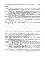
7. References
Chang, C C. ; Kuo, Y.u-F. ; Wang, J C. & Chen, S L. (2010). Air Cooling for a Large Scale
Motor. Applied Thermal Engineering, Vol. 30, Issue 11-12, pp.1360-1368.
Chang, Y W. ; Cheng, C H. ; Wang, J C. & Chen, S L. (2008). Heat Pipe for Cooling
of Electronic Equipment. Energy Conversion and Management, Vol. 49, pp.3398-
3404.
Chang, Y W.; Chang, C C.; Ke, M T. & Chen, S L. (2009). Thermoelectric air-cooling
module for electronic devices. Applied Thermal Engineering, Vol. 29, No. 13, pp.2731-
2737.
Chen, S L.; Chang, C C.; Cheng, C H. & Ke, M T. (2009). Experimental and numerical
investigations of air cooling for a large-scale motor. International Journal of Rotating
Machinery, Vol. 2009, Article ID 612723, 7 pages.
Huang, H S.; Weng, Y C.; Chang, Y W.; Chen, S L. & Ke, M T. (2010). Thermoelectric
water-cooling device applied to electronic equipment. International Communications
in Heat and Mass Transfer, Vol. 37, No. 2, pp.140-146.
Lin, V. & Chen, S L. (2003). Performance analysis, optimum and verification for parallel
plate heat sink associated with single non-uniform heat source, ASME 2003
International Electronic Packaging Technical Conference and Exhibition, InterPACK2003,

Vol. 2, pp.229-236.
Tsai, T E.; Wu, G W.; Chang, C C; Shih, W P. & Chen, S L. (2010a). Dynamic test method
for determining the thermal performances of heat pipes. International Journal of Heat
and Mass Transfer, Vol. 53, No. 21-22, pp.4567-4578.

Air Cooling Module Applications to Consumer-Electronic Products

365
Tsai, T E.; Wu, H H.; Chang, C C. & Chen, S L. (2010b). Two-phase closed thermosyphon
vapor-chamber system for electronic cooling. International Communications in Heat
and Mass Transfer, Vol. 37, No. 5, pp.484-489.
Tsai, Y P. ; Wang, J C. & Hsu, R Q. (2011). The Effect of Vapor Chamber in an Injection
Molding Process on Part Tensile Strength. EXPERIMENTAL TECHNIQUES, Vol.
35, Issue 1, pp.60-64.
Wang R T. & Wang, J C. (2011a). Green Illumination Techniques applying LEDs Lighting,
Proceedings of GETM 2011 May 28, pp.1-7, Changhua, Taiwan.
Wang, J C. & Chen, T C. (2009). Vapor chamber in high performance server. Microsystems
IEEE 2010 Packaging Assembly and Circuits Technology Conference (IMPACT), 2009 4th
International, pp.364-367.
Wang, J C. & Huang, C L. (2010). Vapor chamber in high power LEDs. IEEE 2011
Microsystems Packaging Assembly and Circuits Technology Conference (IMPACT), 2010
5th International, pp.1-4.
Wang, J C. & Tsai,Y P. (2011). Analysis for Diving Regulator of Manufacturing Process.
Advanced Materials Research, Vol. 213, pp.68-72.
Wang, J C. & Wang R T. (2011b). A Novel Formula for Effective Thermal Conductivity of
Vapor Chamber, EXPERIMENTAL TECHNIQUES, DOI : 10.1111/j.1747-
1567.2010.00652.x, early view.
Wang, J C. (2009). Superposition Method to Investigate the Thermal Performance of Heat
Sink with Embedded Heat Pipes. International Communication in Heat and Mass
Transfer, Vol. 36, Issue 7, pp.686-692.

Wang, J C. (2008). Novel Thermal Resistance Network Analysis of Heat Sink with
Embedded Heat Pipes. Jordan Journal of Mechanical and Industrial Engineering, Vol. 2,
No. 1, , pp. 23-30.
Wang, J C. (2010). Development of Vapour Chamber-based VGA Thermal Module.
International Journal of Numerical Methods for Heat & Fluid Flow, Vol. 20, Issue 4,
pp.416-428.
Wang, J C. (2011a). Investigations on Non-Condensation Gas of a Heat Pipe. Engineering,
Vol. 3, pp.376-383.
Wang, J C. (2011b). L-type Heat Pipes Application in Electronic Cooling System.
International Journal of Thermal Sciences, Vol. 50, Issue 1, pp.97-105.
Wang, J C. (2011c). Applied Vapor Chambers on Non-uniform Thermo Physical
Conditions. Applied Physics, Vol. 1, pp.20-26.
Wang, J C. (2011d). Thermal Investigations on LEDs Vapor Chamber-Based Plates.
International Communication in Heat and Mass Transfer, DOI :
10.1016/j.icheatmasstransfer.2011.07.002, Article in Press, Corrected Proof.
Wang, J C. ; Huang, H S. & Chen, S L. (2007). Experimental Investigations of Thermal
Resistance of a Heat Sink with Horizontal Embedded Heat Pipes, International
Communications in Heat and Mass Transfer, Vol. 34, Issue 8, pp.958-970.
Wang, J C. ; Wang, R T. ; Chang, C C. & Huang, C L. (2010a). Program for Rapid
Computation of the Thermal Performance of a Heat Sink with Embedded Heat
Pipes. Journal of the Chinese Society of Mechanical Engineers, Vol. 31, Issue 1, pp.21-
28.

Heat Transfer – Engineering Applications

366
Wang, J C. ; Wang, R T.; Chang, T L. & Hwang, D S. (2010b). Development of 30 Watt
High-Power LEDs Vapor Chamber-Based Plate. International Journal of Heat and
Mass Transfer, Vol. 53, Issue 19/20, pp.3900-4001.
Wang, J C.; Chang T L. ; Tsai Y P. ; & Hsu R Q. (2011a). Experimental Analysis for

Thermal Performance of a Vapor Chamber Applied to High-Performance
Servers, Journal of Marine Science and Technology-Taiwan, Article in Press,
Corrected Proof.
Wang, J C.; Li, A T.; Tsai,Y P. & Hsu, R Q. (2011b). Analysis for Diving Regulator
Applying Local Heating Mechanism of Vapor Chamber in Insert Molding
Process. International Communication in Heat and Mass Transfer, Vol.38, Issue 2,
pp.179-183.
Wu, H H.; Hsiao, Y Y.; Huang, H S.; Tang, P H. & Chen, S L. (2011). A practical plate-fin
heat sink model. Applied Thermal Engineering, Vol.31, Issue 5, pp.984-992.
15
Design of Electronic Equipment Casings
for Natural Air Cooling: Effects of Height
and Size of Outlet Vent on Flow Resistance
Masaru Ishizuka and Tomoyuki Hatakeyama
Toyama Prefectural University
Japan
1. Introduction
As the power dissipation density of electronic equipment has continued to increase, it has
become necessary to consider the cooling design of electronic equipment in order to develop
suitable cooling techniques. Almost all electronic equipment is cooled by air convection. Of
the various cooling systems available, natural air cooling is often used for applications for
which high reliability is essential, such as telecommunications. The main advantage of
natural convection is that no fan or blower is required, because air movement is generated
by density differences in the presence of gravity. The optimum thermal design of electronic
devices cooled by natural convection depends on an accurate choice of geometrical
configuration and the best distribution of heat sources to promote the flow rate that
minimizes temperature rises inside the casings. Although the literature covers natural
convection heat transfer in simple geometries, few experiments relate to enclosures such as
those used in electronic equipment, in which heat transfer and fluid flow are generally
complicated and three dimensional, making experimental modeling necessary. Guglielmini

et al. (1988) reported on the natural air cooling of electronic boards in ventilated enclosures.
Misale (1993) reported the influence of vent geometry on the natural air cooling of vertical
circuit boards packed within a ventilated enclosure. Lin and Armfield (2001) studied
natural convection cooling of rectangular and cylindrical containers. Ishizuka et al. (1986)
and Ishizuka (1998) presented a simplified set of equations derived from data on natural air
cooling of electronic equipment casings and showed its validity. However, there is
insufficient information regading thermal design of practical electronic equipment. For
example, the simplified set of equations was based on a ventilation model like a chimney
with a heater at the base and an outlet vent on the top, yet in practical electronic equipment,
the outlet vent is located at the upper part of the side walls, and the duct is not circular.
Therefore, here, we studied the effect of the distance between the outlet vent location and
the heat source on the cooling capability of natural-air-cooled electronic equipment casings.
2. Set of equations
Ishizuka et al. (1986) proposed the following set of equations for engineering applications in
the thermal design of electronic equipment:

Heat Transfer – Engineering Applications

368
= 1.78 + 300
1.25 0.5 1.5
eq. m o o
QS T A(h/K) T (1)
= 2.5(1 - )/
2
K

 (2)

= 1.3

om
T T (3)

= + 1 / 2
e
q
.to
p
side bottom
SS + S S (4)
where Q denotes the total heat generated by the components, S
eq
is the equivalent total
surface of the casing,
T
m
is the average temperature rise in the casing, A
o
is the outlet vent
area of the casing, h is the distance from the heater position to the outlet, K is the flow
resistance coefficient arising from air path interruption at the outlet,
T
o
is the air
temperature rise at the outlet vent, and
 is the porosity coefficient of the outlet vent. K was
approximated as a function of
: Ishizuka et al. (1986, 1987) obtained the following relation
for wire nets at low values of the Reynolds number (Re):



2 -0.95
=40( 1- / )KRe
(5)
where Re is defined on the basis of the wire diameter used in the wire nets. However, since
the effect of Re on K is less prominent than that of
, K can be approximated as a function of
 only. Therefore, Eq. (2) is considered to be a reasonable expression for practical
applications. The h term in Eq. (1) refers to chimney height, as Eq. (1) assumes a ventilation
model like a chimney with a heater at the base and an outlet vent on the top (Fig. 1).
However, as practical electronic equipment is nothing like a chimney, we took practical
details into account in the following experiments.


Fig. 1. Ventilation model
3. Experiments
3.1 Experimental apparatus
The experimental casing measured 220 mm long  230 mm wide  310 mm high (Fig. 2). The
plastic casing material was 10 mm thick and had a thermal conductivity of 0.01 W/(m·K). A
wire heater (2.3-mm gauge) was placed inside (Fig. 3). The size, location, and grille
patterning of a rectangular vent on one of the side walls were varied (Fig. 4). Experiments
Design of Electronic Equipment Casings for Natural Air Cooling:
Effects of Height and Size of Outlet Vent on Flow Resistance

369

Fig. 2. Experimental casing

Fig. 3. Heater construction
were performed for three distances between the wall base and the center of the outlet vent
(H
v
= 275, 200, and 150 mm) and for three heights of the heater above the base (H
h
= 25,
125, and 225 mm), with the heater always placed below the outlet vent. The cooling air
entered through an opening in the center of the casing base (150 mm
 130 mm) and was
exhausted through the upper outlet. The air temperature distribution inside the casing,
the room temperature, and the wall temperatures were measured by calibrated K-type
thermocouples (±0.1 K, 0.1 mm in diameter). The thermocouples inside the casing were
arranged 30, 85, and 115 mm from the inside of the left side wall at each of 75, 175, and
275 mm above the base (Fig. 2). On the walls, thermocouples were placed at the center of

Heat Transfer – Engineering Applications

370
the top surface and at three locations down the center line of each side wall, and one
thermocouple was placed outside the casing to measure the room temperature. The mean
inner air temperature rise,
T
m
, was calculated from the locally measured values over the
whole volume of the casing.


Fig. 4. Outlet vent openings
3.2 Estimation of heat removed from casing surfaces

The amount of heat removed from the casing surfaces was estimated by experiment. For this
purpose, the casing was considered to be a closed unit with no vents except at the base. Using
the natural convective heat transfer equations for individual surfaces presented by Ishizuka et
al. (1986), we expressed the amount of heat removed from the casing surfaces, Q
s
, as:

1.25
=
s1m
QDT (6)
Design of Electronic Equipment Casings for Natural Air Cooling:
Effects of Height and Size of Outlet Vent on Flow Resistance

371
Eq. (6) shows the first term on the right-hand side of Eq. (1). Where, D
1
is the constant
coefficient. The coefficient D
1
includes a radiative heat transfer factor and determined by the
experiment. The amount of heat generation was within the Q
s
= 6–40 W range (Fig. 5) when
the room temperature T
a
was 298 K. The results are shown in Fig.5 and are well expressed
by Eq.(7).

1 .25

=0.445
sm
QT (7)
where D
1
was determined to be 0.445. The temperature distribution in the casing was
relatively uniform, within ±5%. Hereafter, the amount of heat removed from the outlet vent,
Q
v
, was calculated as:


vs
Q= Q - Q (8)





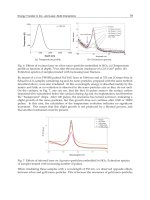
Fig. 5. Relationship between Q
s
and T
m

3.3 Influence of outlet vent size on temperature rise in the casing
The experiment was carried out by varying the outlet vent size of the reference casing at
outlet vent position H
v
= 275 mm and heater position at H
h

= 25 mm (Fig. 2). The porosity
coefficient 
o
(Fig. 4) was defined as the ratio of the open area of each individual vent to the
area of the reference vent (150 mm  50 mm).
At each value of input power, Q, as 
o
decreased, T
m
increased linearly on the logarithmic
plot (Fig. 6). As Q increased, T
m
also increased.
3.4 Influence of outlet vent position on mean temperature rise in the casing
The relationship between T
m
and outlet vent position H was investigated at two opening
sizes with the heater at the bottom. T
m
decreased as H increased at both opening sizes (Fig.
7). It decreased faster at lower H.

Heat Transfer – Engineering Applications

372

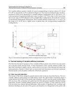
Fig. 6. Influence of vent porosity and input power on mean temperature rise in the casing


Fig. 7. Influence of outlet vent position on mean temperature rise in the casing

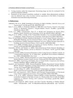
3.5 Influence of distance between outlet vent position and heater position on mean
temperature rise in the casing
The relationship between T
m
(average of temperatures measured only above the heater
position) and the distance between the outlet vent position and the heater position, h, was
investigated by varying opening size and input power while the outlet height was fixed at
H
v
= 275 mm. As h increased, T
m
decreased at all values of input power (Fig. 8).
Design of Electronic Equipment Casings for Natural Air Cooling:
Effects of Height and Size of Outlet Vent on Flow Resistance

373

Fig. 8. Influence of distance between outlet vent position and heater position on mean
temperature rise in the casing
4. Correlations using non-dimensional parameters
4.1 Flow resistance coefficient K
The flow resistance coefficient K was related to Q
v
and h. If we assume a uniform
temperature distribution and a one-dimensional steady-state flow in a ventilation model as
shown in Fig. 1, we can express Eq. (9) for the overall energy balance and Eq. (10) for the
balance between flow resistance and buoyancy force:

vp
Q = cAu T



(9)

2
g/2
a
( - ) h = K u
 
(10)
where Q
v
is dissipated power, c
p
is specific heat of the air at constant pressure, A is the
cross-sectional area of the duct, u is airflow velocity, T is temperature rise,  is air
density (
a
is atmospheric condition), g is acceleration due to gravity, h is the distance
between the outlet and the heater, and K is the flow resistance coefficient for the system.
Since the pressure change in the system is small, the expression can be rewritten to
assume a perfect gas:

()/ =()/
aaa
- T - T T
 
(11)
K is defined in terms of hand Q
v

as:

3 2
v
= 2
g
/ ( ( / ) )
ap
Kh TT cAQ

 (12)
In this study, H value was used in spite of h to arrange the present data.