Human Musculoskeletal Biomechanics Part 2 doc

A Task-level Biomechanical Framework for Motion Analysis and Control Synthesis 9
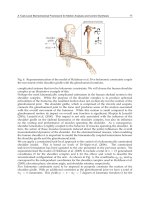
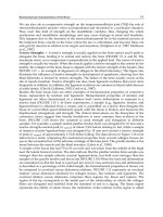
Fig. 6. Reparameterization of the model of Holzbaur et al. Five holonomic constraints couple
the movement of the shoulder girdle with the glenohumeral rotations.
complicated systems that involve holonomic constraints. We will choose the human shoulder
complex as an illustrative example of this.
Perhaps the most kinematically complicated subsystem in the human skeletal system is the
shoulder complex. While the purpose of the shoulder complex is to produce spherical
articulation of the humerus, the resultant motion does not exclusively involve motion of the
glenohumeral joint. The shoulder girdle, which is comprised of the clavicle and scapula,
connects the glenohumeral joint to the torso and produces some of the motion associated
with the overall movement of the humerus. While this motion is small compared to the
glenohumeral motion its impact on overall arm function is significant, Klopˇcar & Lenarˇciˇc
(2001); Lenarˇciˇc et al. (2000). This impact is not only associated with the influence of the
shoulder girdle on the skeletal kinematics of the shoulder complex, but also its influence
on the routing and performance of muscles spanning the shoulder. As a consequence,
shoulder kinematics is tightly coupled to the behavior of muscles spanning the shoulder. In
turn, the action of these muscles (moments induced about the joints) influences the overall
musculoskeletal dynamics of the shoulder. For the aforementioned reasons, when modeling
the human shoulder it is important to model the kinematically coupled interactions between
the shoulder girdle and the glenohumeral joint.
We can apply a constrained task-level approach to the control of a holonomically constrained
shoulder model. This is based on work of De Sapio et al. (2006). The constrained
task-level formulation has been updated to the one presented in the previous section. We
reparameterized the model of Holzbaur et al. (2005) to include a total of n
= 13 generalized
coordinates (9 for the shoulder complex and 4 for the elbow and wrist) to describe the
unconstrained configuration of the arm. As shown in Fig. 6, the coordinates q
6
, q
7
,andq

9
correspond to the independent coordinates for the shoulder complex used in Holzbaur et al.
(2005); elevation plane, elevation angle, and shoulder rotation, respectively.
Five holonomic constraints need to be imposed to properly constrain the motion of the
shoulder girdle. With an additional constraint at the glenohumeral joint we have a total of
m
C
= 6 constraints. This yields p = n − m
C
= 7 degrees of kinematic freedom (3 for the
11
A Task-Level Biomechanical Framework for Motion Analysis and Control Synthesis
10 Will-be-set-by-IN-TECH
shoulder complex and 4 for the elbow and wrist). These constraint equations, φ(q)=0,are
given by.
φ
(q)=
⎛
⎜
⎜
⎜
⎜
⎜
⎜
⎜
⎜
⎜
⎝
q
1

− b
1
q
6
− c
1
q
7
q
2
− b
2
q
6
− c
2
q
7
q
3
− b
3
q
6
− c
3
q
7
q
4

− b
4
q
6
− c
4
q
7
q
5
− b
5
q
6
− c
5
q
7
q
8
+ q
6
⎞
⎟
⎟
⎟
⎟
⎟
⎟
⎟

⎟
⎟
⎠
= 0, (37)
where the constraint constants, b and c, associated with the dependency on humerus elevation
plane and elevation angle were obtained from the regression analysis of de Groot and Brand
de Groot & Brand (2001).
2.4 Simulated control implementation
Defining a humeral orientation, or pointing, task we have,
x
(q)=

q
6
q
7
q
9

T
. (38)
We will not control any of the constraint forces so our control equations consist of,
τ
+ Φ
T
λ =

Θ
T
J

T
(

Λ
c
f

+ μ
c
+ p
c
)+Φ
T
( α + ρ)+

N
T
c
τ
o
, (39)
f

= K
p
(x
d
− x)+K
v
( ˙x

d
− ˙x)+¨x
d
, (40)
S
p
τ = 0, (41)
where S
p
accounts for the unactuated (passive) joints, q
1
, ··· , q
5
,andq
8
,
S
p
=
⎛
⎜
⎜
⎜
⎜
⎜
⎜
⎜
⎜
⎜
⎜

⎜
⎜
⎝
100000000
010000000
001000000
000100000
000010000
000000010
⎞
⎟
⎟
⎟
⎟
⎟
⎟
⎟
⎟
⎟
⎟
⎟
⎟
⎠
. (42)
Fig. 7 displays simulation plots for the shoulder complex under a goal position command. The
controller was applied to both the constrained shoulder model and a simple model with only
glenohumeral articulation (motion of the scapula and clavicle not coupled to glenohumeral
motion). The glenohumeral joint control torques associated with the constrained and simple
shoulder models, performing identical humeral pointing tasks, differ over their respective
time histories. This is particularly true for shoulder elevation angle and elevation plane.

2.5 Muscle-based actuation
In the previous section the simulation of the shoulder complex was actuated with joint torque
actuators. In reality biomechanical systems are actuated by a set of musculotendon actuators.
Hill-type lumped parameter models for muscle-tendon pairs yield equations of state which
12
Human Musculoskeletal Biomechanics
A Task-level Biomechanical Framework for Motion Analysis and Control Synthesis 11
Fig. 7. (Top) Time response of humeral pointing during execution of a goal command for
constrained and simple shoulder models. Appropriate dynamic compensation accounts for
the control task, x, and the shoulder girdle constraints, φ. The control gains are k
p
= 100 and
k
v
= 20. (Bottom) Glenohumeral joint control torques as predicted by the constrained and
simple shoulder models. The inclusion of shoulder girdle constraints influences the resulting
torques, particularly for shoulder elevation plane, q
6
, and elevation angle, q
7
.
describe musculotendon behavior, Zajac (1993). Given a set of r musculotendon actuators we
can express the vector of musculotendon forces as f
= f (l,
˙
l, a) ∈ R
r
,wherel ∈ R
r
are the

muscle lengths whose behavior is described by a state equation and a
∈ R
r
are the muscle
activations, which reflect the level of motor unit recruitment for a given muscle. Activation is
a normalized quantity, that is a
i
∈ [0, 1]. By using either a stiff tendon model or a steady state
evaluation of the musculotendon forces we can express f
= f (q,˙q, a)=F (q,˙q)a,where
F
(q,˙q) ∈ R
r×r
is a diagonal matrix mapping muscle activation, a, to muscle force, f .The
joint moments induced by these musculotendon forces are,
τ
= −L(q)
T
f = −L(q)
T
F (q,˙q)a = B(q,˙q)
T
a, (43)
where L
(q)=∂l/∂q ∈ R
r×n
is the musculotendon path Jacobian and B(q,˙q)
T
∈ R
n×r

maps
muscle activation, a,tojointtorque,τ . Equation (5) can thus be expressed in terms of muscle
actuation,
M ¨q
+ b + g − Φ
T
λ = B
T
a. (44)
We can then express the control equation as (26),
¯
J
T

Θ
T
B
T
a =

Λf

+ μ + p −
¯
J
T
Φ
T
( α + ρ). (45)
13

A Task-Level Biomechanical Framework for Motion Analysis and Control Synthesis
12 Will-be-set-by-IN-TECH
Fig. 8. Muscle paths spanning the shoulder complex. Muscle moment arms are determined
from the muscle path data Holzbaur et al. (2005). The motion of the shoulder girdle
influences the moment arms about the glenohumeral joint.
Due to both kinematic redundancy and actuator redundancy there will typically be many
solutions for a. Using a static optimization procedure, Thelen et al. (2003), this can be
resolved by finding the solution which minimizes

a

2
given a
i
∈ [0, 1]. This corresponds to
minimizing the instantaneous muscle effort. The use of

a

2
and similar cost measures have
been suggested in a number of sources, Anderson & Pandy (2001); Crowninshield & Brand
(1981).
In Section 2.4 we observed that the constrained shoulder model, which involves kinematic
coupling between the humerus, scapula and clavicle, differs from the simple shoulder model
with regard to the control torques that are required to achieve a desired motion control task.
The constrained model also differs from the simple model in the degree to which the system
of muscles are able to generate control forces to achieve a desired motion control task. This is
due to the influence of the constrained motion between the humerus, scapula and clavicle on
the muscle forces and muscle moment arms about the glenohumeral joint (see Fig. 8).

An example of this is shown in Fig. 9. Predicted muscle moment arms, muscle forces,
and moment generating capacities for the deltoid muscles are compared for the simple
and constrained shoulder models. The muscle path and force-length data were taken from
the study of Holzbaur et al. (2005). In the constrained shoulder model the motions of the
scapula and clavicle are highly coupled to humerus elevation angle (q
7
coordinate), whereas,
in the simple shoulder model the motion of the scapula and clavicle are not coupled to
glenohumeral motion. The paths of the deltoid muscles are affected by the constrained motion
of the humerus, scapula, and clavicle. This results in significant differences in moment arms
predicted by the two models, with the constrained model often generating moment arms of
substantially larger magnitude than the simple model.
Additionally, the predicted isometric muscle forces (computed at full activation) generated by
the two models differ. The resulting moment generating capacities of the constrained model
are often substantially larger in magnitude than the simple model. This implies that the simple
model, which excludes the constrained shoulder girdle motion, typically underestimates the
moment generating capacities of muscles that span the shoulder, since Holzbaur et al. (2005)
demonstrated correlation between predicted and experimental moment generating capacities
14
Human Musculoskeletal Biomechanics
A Task-level Biomechanical Framework for Motion Analysis and Control Synthesis 13
Fig. 9. (Top) Muscle moment arms for the deltoid muscles, as predicted by the constrained
and simple shoulder models. The constrained model typically generates moment arms of
substantially larger magnitude than those of the simple model. (Bottom) Muscle forces and
moment generating capacities for the deltoid muscles. The resulting moment generating
capacities associated with the constrained model are typically larger in magnitude than those
associated with the simple model.
for the constrained model. This is critical in various applications involving the study and
synthesis of human movement, Khatib et al. (2004).
3. Posture-based modeling and analysis of biomechanical systems

In this section we present a muscle effort criterion for the prediction of upper limb postures.
In the overall framework this addresses the highlighted element of Fig. 10. The focus is
on developing a neuromuscular criterion and a methodology for synthesizing posture in the
presence of that criterion.
A particularly relevant class of human movements involves targeted reaching. Given a
specific target the prediction of kinematically redundant upper limb motion is a problem of
choosing one of a multitude of control solutions, all of which yield kinematically feasible
configurations. It has been observed that humans resolve this redundancy problem in a
relatively consistent manner, Kang et al. (2005); Lacquaniti & Soechting (1982). For this reason
general mathematical models have proven to be valuable tools for motor control prediction
across human subjects.
Approaches for predicting human arm movement have been categorized into posture-based
and trajectory-based (or transport-based) models, Hermens & Gielen (2004); Vetter et al.
(2002). Posture-based models are predicated upon the assumption of Donders’ law.
Specifically, Donders’ law postulates that final arm configuration is dependent only on
15
A Task-Level Biomechanical Framework for Motion Analysis and Control Synthesis
14 Will-be-set-by-IN-TECH
Fig. 10. Task/posture motion control model for biomechanical systems highlighting posture
control from neuromuscular criteria.
final hand position and is independent of initial (or past) arm configurations. Thus, the
fundamental characteristic of posture-based models is path independence in predicting
equilibrium arm postures. In these models the postulated behavior of the central nervous
system (CNS) can be said to execute movements based strictly on control variables (e.g.,
hand position). Conversely, trajectory-based models, which include the minimum work
model, Soechting et al. (1995), and the minimum torque-change model, Uno et al. (1989), are
characterized by dependence of final arm configuration on the final hand position, the starting
configuration, and the choice of a specific optimal path parameterized over time (i.e., past arm
configurations).
Many of the models for predicting human arm movement, including the minimum work

model and the minimum torque-change model, do not involve any direct inclusion of
muscular properties such as routing kinematics and strength properties. Even models
described as employing biomechanical variables, Kang et al. (2005), typically employ only
variables derivable purely from skeletal kinematics and not musculoskeletal physiology. It is
felt that the utilization of a model-based characterization of muscle systems, which accounts
for muscle kinematic and strength properties, is critical to authentically simulating human
motion since all human motion is predicated upon physiological capabilities.
3.1 Biomechanical effort minimization
We begin with a general consideration of biomechanical effort measures. An instantaneous
effort measure can be used in a trajectory-based model of movement by seeking a trajectory,
consistent with task constraints, that minimizes the integral of that measure over the
time interval of motion. Alternatively, the instantaneous effort measure can be used in a
posture-based model by seeking a static posture, consistent with the target constraint, which
minimizes the static form of the measure.
Proceeding from Section 2.5 we express the joint torques in terms of muscle activations,
τ
= −L(q)
T
f = −L(q)
T
F (q,˙q)a = B(q,˙q)
T
a. (46)
Due to the fact that there are typically more muscles spanning a set of joints than the number
of generalized coordinates used to describe those joints this equation will have an infinite set
of solutions for a. Choosing the solution, a
o
, which has the smallest magnitude (least norm)
yields,
a

o
= B
T+
τ = B(B
T
B)
−1
τ , (47)
16
Human Musculoskeletal Biomechanics
A Task-level Biomechanical Framework for Motion Analysis and Control Synthesis 15
where B
T+
is the pseudoinverse of B
T
. Our instantaneous muscle effort measure can then
be expressed as,
U
=

a
o

2
= τ
T
(B
T
B)
−1

τ . (48)
Expressing this effort measure in constituent terms and dissecting the structure we have,
U
= τ
T
muscular capacity
  
[ L
T

kinematics
(FF
T
)
  
kinetics
L

kinematics
]
−1
τ . (49)
This allows us to gain some physical insight into what is being measured. The terms inside the
brackets represent a measure of the net capacity of the muscles. This is a combination of the
force generating kinetics of the muscles as well as the mechanical advantage of the muscles,
as determined by the muscle routing kinematics. The terms outside of the brackets represent
the kinetic torque requirements of the task and posture.
It is noted that the solution of (46) expressed in (47) corresponds to a constrained minimization
of


a

2
, however, this solution does not enforce the constraint that muscle activation must be
positive (muscles can only produce tensile forces). Imposing inequality constraints, 0
≤ a
i
≤
1, on the activations requires a quadratic programming (QP) approach for performing the
constrained minimization. In this case the solution of (46) which minimizes

a

2
and satisfies
0
≤ a
i
≤ 1 can be represented in shorthand as,
a
o
= QP(B
T
, τ ,

a

2
,0≤ a
i

≤ 1), (50)
where QP
(

) represents the output of a quadratic programming function (e.g., quadprog()
in the Matlab optimization toolbox). Our muscle effort criterion is then U
=

a
o

2
,where
a
o
is given by (50). Despite the preferred use of quadratic programming for computational
purposes, (49) provides valuable insights at a conceptual level.
3.2 Posture-based criteria
For posture-based analysis the static form of the instantaneous muscle effort measure can be
constructed by noting that ˙q
→ 0, thus eliminating the dependency of U on ˙q.Thisalso
implies that τ
→ g. Thus, the static form, U(q), of (48) is,
U
(q)=g(q)
T
[B(q)
T
B(q)
T

]
−1
g(q). (51)
Alternatively, imposing the inequality constraints on the activations we have U
=

a
o

2
where,
a
o
= QP(B( q)
T
, g(q),

a

2
,0≤ a
i
≤ 1). (52)
To find a task consistent static configuration which minimizes U
(q),wefirstdefinethe
self-motion manifold associated with a fixed task point, x
o
. ThisisgivenbyM(x
o
)=

{
q | x(q)=x
o
} where x(q) is the operational point of the kinematic chain (e.g., the position
of the hand). For each q on M
(x
o
) we can compute U(q)=

a
o

2
by solving the quadratic
programming problem of (52). The minimal effort task consistent configuration is then the
configuration, q,forwhichU
(q) is minimized on M(x
o
). Figure 11 illustrates changes in the
predicted posture associated with minimal muscle effort as weight at the hand is varied.
17
A Task-Level Biomechanical Framework for Motion Analysis and Control Synthesis
16 Will-be-set-by-IN-TECH
Fig. 11. Muscle effort variation and predicted minimal efforts associated with different
weights in hand. The weight at the hand was projected into joint space and added to the
gravity vector associated with the limb segments. The effect is that the predicted posture,
associated with the minimum of the muscle effort curve, shifts as weight is added. Each
point on each of the curves was computed by solving a quadratic programming problem.
3.3 Sphere methods for quadratic programming
Quadratic programming addresses the general minimization of a quadratic function subject

to a combination of equality and inequality constraints. It can be formally stated as:
Minimize the objective function, z
(x),withrespecttox,where,
z
(x)=
1
2
x
T
Dx + d
T
x, (53)
subject to,
Ax
≥ b, (54)
Cx
= y. (55)
We assume that D is symmetric positive definite and that the polytope defined by Ax
≥ b is
convex. In the case of muscle effort minimization we have the specific form,
z
(a)=
1
2
a
T
a, (56)
subject to,

1

r×r
−1
r×r

a
≥

0
r×1
−1
r×1

(57)
B
(q)
T
a = g(q), (58)
where 1
r×r
is the r × r identity matrix, 0
r×1
is a column vector of zeros,and1
r×1
is a column
vector of ones. Clearly, the quadratic form (56) is positive definite and the polytope (57) is
convex. For the procedure of muscle effort minimization this QP problem is repeatedly solved
for different values of q on M
(x
o
), generating the function U(q). A line search over M(x

o
)
then yields q
o
where U(q
o
) represents the minimum of U on the self-motion manifold.
18
Human Musculoskeletal Biomechanics
A Task-level Biomechanical Framework for Motion Analysis and Control Synthesis 17
Since this QP problem needs to be solved repeatedly we would like an efficient method for
solving it. There are a number of interior point method (IPM) solvers that addresses QP
problems. We have implemented one based on the sphere method approach. This approach
was initially developed for linear programming (LP) problems, Murty (2006); Murty (2010b),
but has been extended for QP problems, Murty (2010a). Our implementation of the sphere
method approach for QP will be described here and is based on the approach of Murty et al.
We begin with the general problem of minimizing (53) subject to (54) and (55). It is noted that
the equality constraints, Cx
= y, can be represented as the inequality constraints.
Cx
> y − , (59)
Cx
< y + . (60)
where  is a vector of small positive tolerances. Consequently, we consider all constraints,
both equality and inequality, as being represented by Ax
≥ b. These constraints describe a
polytope K. A simple check can be made to determine if the unconstrained minimum of the
objective function is interior to the polytope. If this is the case then the solution to the QP
problem is trivial. Assuming that this is not the case we proceed by noting that the facetal
hyperplanes defined by, Ax

= b, can be represented as,
v
T
i
x = b
i
for i = 1, ··· , m, (61)
where
{v
1
, ··· , v
m
} are the inward normals of the facetal planes and,
A
=
⎛
⎜
⎝
v
T
1
.
.
.
v
T
m
⎞
⎟
⎠

. (62)
We normalize (61) by dividing both sides by

v
i

.Thus,
ˆv
i
=
v
i

v
i

,
ˆ
b
i
=
b
i

v
i

,
ˆ
A =

⎛
⎜
⎝
ˆv
T
1
.
.
.
ˆv
T
m
⎞
⎟
⎠
. (63)
Following these normalizations we perform centering steps from some initial point, x
i
,
interior to the polytope. Two types of centering steps are performed. One is termed a
line search from facetal normals (LSFN), the other is termed a line search from computed
profitable directions (LSCPD). First, the touching set, T
(x),atthecurrentpoint,x (initially
x
i
) is computed. This is the set of facetal hyperplanes which are touched by the largest
hypersphere that can be inscribed in the polytope, centered at the current point, x.
For the LSFN step the facetal unit normals,
{ ˆv
1

, ··· ,ˆv
m
}, are iterated through until one is
found, ˆy, such that,
ˆv
T
i
ˆy > 0foralli ∈ T(x), (64)
and such that it reduces the objective function, that is,
− [∇z(x)]
T
ˆy > 0, (65)
where
∇z(x)=Dx + d. Given a profitable direction, ˆy, that meets these criteria a line
search is performed to move along this profitable direction until a point is reached for which
19
A Task-Level Biomechanical Framework for Motion Analysis and Control Synthesis
18 Will-be-set-by-IN-TECH
the inscribed sphere at that point is a maximum. A backtracking line search has been
implemented for this. The line search is terminated at any point where (65) is not satisfied
(no longer descending). This LSFN step is repeated as long as profitable directions meeting
the criteria are found.
For the LSCPD step the linear system,
ˆv
T
i
y
1
= 1and − [∇z(x)]
T

y
1
= 0foralli ∈ T(x), (66)
is solved for a direction y
1
and the linear system,
ˆv
T
i
y
2
= 0and − [∇z(x)]
T
y
2
= 1foralli ∈ T(x), (67)
is solved for a direction y
2
. Backtracking line searches are performed sequentially in both
of these unit directions, ˆy
1
and ˆy
2
, until a point is reached for which the inscribed sphere at
that point is a maximum. Again, the line search is terminated at any point where (65) is not
satisfied. This LSCPD step is repeated until the incremental reduction in the objective function
falls below some tolerance. The final output of the centering steps will be labeled x
r
.
Following the centering steps, descent steps are performed. For a given iteration, a single

descent step is chosen based on the best performance of a set different descent steps, in
reducing the objective function. All of these descent steps terminate at the boundary of the
polytope. Given a unit descent direction ˆy the distance along this direction to the polytope
boundary is given by,
δ
= min

ˆv
T
i
x
r
−
ˆ
b
i
ˆv
T
i
ˆy

over i, such that, ˆv
T
i
ˆy < 0. (68)
These candidate descent directions are as follows:
• D1: Choose y
= −∇z(x
r
).Movefromx

r
along ˆy to the boundary of K.
• D2: Choose y to be the direction defined by the displacement vector between the previous
two centering locations, y
= x
r
− x
r−1
.Movefromx
r
along ˆy to the boundary of K.
• D3: Define directions associated with projecting
−∇z(x
r
) on each of the facetal
hyperplanes in the touching set. These directions are given by,
y
i
= −(1 − ˆv
i
ˆv
T
i
)∇z(x
r
) ∀i ∈ T(x
r
). (69)
Move from x
r

along ˆy
i
, ∀i ∈ T(x
r
),totheboundaryofK.Ofthese|T(x
r
)| descents retain
the one that results in the greatest reduction in the objective function.
• D4: Choose y to be the average of the directions from D3. Move from x
r
along ˆy to the
boundary of K. The average of the directions from D3 is given by,
y
=
∑
i∈T(x
r
)
−(1 − ˆv
i
ˆv
T
i
)∇z(x
r
)
|T(x
r
)|
. (70)

• D5: Compute the touching point, x
i
r
associated with x
r
. This is the point on each facetal
hyperplane in the touching set where the maximum inscribed hypersphere, centered at x
r
,
touches. These points are given by,
x
i
r
= x
r
+ ˆv
i
(b
i
− ˆv
T
i
x
r
) ∀i ∈ T(x
r
). (71)
20
Human Musculoskeletal Biomechanics
A Task-level Biomechanical Framework for Motion Analysis and Control Synthesis 19

The near touching point is defined as a point on the line segment between x
r
and x
i
r
.
˜x
i
r
= x
r
+(1 − )x
i
r
∀i ∈ T(x
r
), (72)
where epsilon is a small tolerance (e.g.,
≈ 0.1). Projecting −∇z( ˜x
i
r
) on each of the facetal
hyperplanes in the touching set yields,
y
i
= −(1 − ˆv
i
ˆv
T
i

)∇z( ˜x
i
r
) ∀i ∈ T(x
r
). (73)
Move from ˜x
i
r
along ˆy
i
, ∀i ∈ T(x
r
),totheboundaryofK.Ofthese|T(x
r
)| descents retain
the one that results in the greatest reduction in the objective function.
The output of D1 through D5 that results in the greatest reduction in the objective function
is used to yield the new point x. The centering and descent steps are repeated until some
solution tolerance is met. In subsequent iterations the feasible set K shrinks based on the
objective tangent hyperplane passing thorough x. That is, the constraints are appended to
include the objective tangent hyperplane passing through the current x,
ˆ
A
=
⎛
⎜
⎜
⎜
⎝

−[∇z(x)]
T
ˆv
T
1
.
.
.
ˆv
T
m
⎞
⎟
⎟
⎟
⎠
and
ˆ
b
=
⎛
⎜
⎜
⎜
⎝
−[∇z(x)]
T
x
ˆ
b

1
.
.
.
ˆ
b
m
⎞
⎟
⎟
⎟
⎠
. (74)
Fig. 12 illustrates some of the general steps for centering and descent in this algorithm. The
algorithm has been implemented in Matlab and in C++ on problems involving thousands of
variables and constraints. It performs favorably in terms of accuracy and speed as compared
with Matlab’s quadprog() IPM routine. Quantitative benchmarking is planned for the
future.
Fig. 12. An illustration of the centering and descent steps associated with the sphere method
implemented for QP problems.
3.4 Least action of cost criteria
We now pose the problem of minimizing a cost criterion subject to a motion control task. This
is detailed in De Sapio et al. (2008). We can perform this for an instantaneous potential-based
21
A Task-Level Biomechanical Framework for Motion Analysis and Control Synthesis
20 Will-be-set-by-IN-TECH
criterion, U(q), by using a gradient descent method in conjunction with the task/posture
decomposition of (13). Given our overall control torque,
τ
= J

T
f + N
T
τ
p
, (75)
the posture term, τ
p
, can be chosen to correspond to the gradient descent, −∂U/∂q,ofour
cost criterion. In this case the equations of motion are,
M ¨q
+ b + g = J
T
f − N
T
∂U
∂q
, (76)
subject to the task ¨x
(q)= ¨x
d
(t). We complement (76) with the task space control law given
by (17) and (19).
Gradient descent seeks to reduce an instantaneous criterion rather than extremize a criterion
over an integration interval. To address this latter case we define the action integral associated
with a cost criterion, as in De Sapio et al. (2008),
I

t
f


t
o
U(q,˙q) dt. (77)
If no task trajectory constraints are specified we have,
δI
= 0,
∀ δ | δq(t
o
)=δq(t
f
)=0.
(78)
Equations (77) and (78) result in the Euler-Lagrange equations,
d
dt
∂U
∂ ˙q
−
∂U
∂q
= 0. (79)
Imposing rheonomic task trajectory constraints, x
(q)=x
d
(t), implies,
δJ
= 0,
∀ δ | δq(t
o

)=δq(t
f
)=0,andJ δq = 0,
(80)
which yields the system,
d
dt
∂U
∂ ˙q
−
∂U
∂q
= J
T
λ, (81)
or,
M
U
¨q + b
U
+ g
U
= J
T
λ, (82)
subject to ¨x
(q)= ¨x
d
(t). Projecting (82) into task space yields the operational space equations
for this system,

Λ
U
(q,˙q) ¨x + μ
U
(q,˙q)+p
U
(q)=λ, (83)
where Λ
U
, μ
U
,andp
U
are analogous to Λ, μ,andp,butwithM, b,andg replaced by M
U
,
b
U
,andg
U
. Applying constraint stabilization, the trajectory constraints can be expressed as,
¨x
= λ

= ¨x
d
(t)+β[ ˙x
d
(t) − ˙x]+α[x
d

(t) − x], (84)
22
Human Musculoskeletal Biomechanics
A Task-level Biomechanical Framework for Motion Analysis and Control Synthesis 21
and the constraint stabilized system is,
λ
= Λ
U
λ

+ μ
U
+ p
U
. (85)
Two examples from De Sapio et al. (2008) can be used to illustrate the approaches described.
First we consider a simplified n
= 3 degree-of-freedom model of the human arm actuated
by r
= 14 muscles. The system is kinematically redundant with respect to the m = 2
degree-of-freedom task of positioning the hand. The muscle attachment and force-length data
were taken from the study of Holzbaur et al. (2005). We wish to control the hand to move to a
target location, x
f
, while minimizing an instantaneous muscle effort criterion defined as,
U
(q)

g
T

(B
T
B)
−1
g, (86)
where B
(q)=−L(q)
T
F (q) and the muscle forces are modeled as f(q, a)=F (q)a,where,
F
= diag

f
o
i
e
−5

l
i
(q )
l
o
i
−1

2

. (87)
The term, f

o
i
, represents the maximum isometric force for the ith muscle and l
o
i
represents the
optimal fiber length for the ith muscle. No task trajectory, x
d
(t), will be specified, just the final
target location, x
f
.
We have the following control equations,
f

= k
p
(x
f
− x) − k
v
˙x, (88)
τ
= J
T
f

+ g −

N

T
(k
e
∂U
∂q
+ k
d
˙q). (89)
In this case no model of the dynamic properties is included in (??). Also, the terms ¨x
d
(t) and
˙x
d
(t) have been omitted in (88) and x
d
(t) has been replaced by the final target location, x
f
,
since the goal is to move to a target location without specifying a trajectory. To the posture
space portion of (89) we have added a dissipative term, k
d
˙q, and a gain, k
e
, on the gradient
descent term. Finally, the gravity vector, g, is perfectly compensated for in the overall control.
Fig. 13 displays time histories of joint motion, hand motion, and muscle effort for a simulation
run. We can see that the controller achieves the final target objective while the null space
control simultaneously seeks to reduce the instantaneous muscle effort (consistent with the
task requirement). It is recalled that no compensation for the dynamics (except for gravity)
was included in (89). Thus, there is no feedback linearization present in the control. Normally,

perfect feedback linearization without explicit trajectory tracking would produce straight line
motion to the goal. In the absence of feedback linearization non-straight line motion results.
We now seek a trajectory which moves the hand to a target location (see Fig. 14), while
extremizing muscle action,
I

t
f

t
o
U(q,˙q) dt. (90)
In this case we will define the instantaneous muscle effort criterion as,
U
(q,˙q)=
r
∑
i=1

l
i
− l
o
i
l
o
i

2
+

r
∑
i=1

˙
l
i
v
o
i

2
+
˙
q
2
3
, (91)
23
A Task-Level Biomechanical Framework for Motion Analysis and Control Synthesis
22 Will-be-set-by-IN-TECH
Fig. 13. A redundant muscle-actuated model of the human arm. Initial and final
configurations, q
(t
o
) and q(t
f
), associated with gradient descent movement to a target, x
f
,

are shown. (Top) Time history of the arm motion to the target. Motion corresponds to
gradient descent of the muscle effort, subject to the task requirement. (Bottom) Time history
of hand trajectory and muscle effort criterion, U
(q)=g
T
(B
T
B)
−1
g, associated with
gradient descent for human arm model. The null space control seeks to reduce the muscle
effort but is also constrained by the task requirement.
where l
o
i
represents the optimal fiber length for the ith muscle and v
o
i
represents the
maximum contraction velocity for the ith muscle.
Under task constraints the system which extremizes the muscle action is given by,
λ

= α(x
f
− x) − β ˙x, (92)
λ
= Λ
U
λ


+ μ
U
+ p
U
. (93)
and (82). The solution yields the muscle action extremizing path between configurations q
(t
o
)
and q(t
f
), given the hand target constraint. Fig. 14 displays time histories of joint motion,
hand motion, and muscle effort for a simulation run. The straight line motion of the hand
results from the feedback linearization employed.
4. Task/posture control for neural prosthetics
If we return to our initial description of the human motor system depicted in Fig. 1 we can
add an outer loop associated with the high-level task reasoning and planning functions of
24
Human Musculoskeletal Biomechanics
A Task-level Biomechanical Framework for Motion Analysis and Control Synthesis 23
Fig. 14. (Top) Time history of the arm motion between configurations q(t
o
) and q(t
f
).
Motion corresponds to extremization of the muscle effort action integral. (Bottom) Time
history of hand trajectory for human arm model and time history of muscle effort criterion
associated with extremizing the action integral of (91).
the brain. This is depicted in Fig. 15. In this abstraction motion control is divided into a

task generative phase and a motor execution phase. The abstraction depicted in Fig. 15 has
relevance not only to the basic understanding of the biomechanics and control of movement
but also to the design of engineered systems that augment physiological systems.
Neural prosthetics and brain-computer interfaces have emerged as compelling technologies
for the inference of cognitive motor intent using neuroimaging techniques. These techniques
can be invasive, as in the case of a brain implant, or non-invasive, as in the case of
electroencephalography (EEG). In either case the goal of these techniques is to restore or
augment a degree of motor functionality to an individual. This is accomplished through
the prediction of motor intent, based on inference from neuroimaging data, and subsequent
realization of that intent through a robotic prosthesis. This inference involves decoding the
neural encoding manifested in the neuroimaging data. As referenced earlier, current research
suggests a task-oriented spatial encoding of motor intent. Based on this premise exciting work
has been done to control robotic devices by decoding motor intent.
Current breakthroughs in motor-based brain-computer interfaces can be furthered by the
implementation of more sophisticated control theoretic algorithms. Using existing invasive
or non-invasive neuroimaging techniques it is believed that the performance of computer
controlled robotic devices can be enhanced using a task/posture control framework where,
in addition to the inference of task-oriented objectives, postural control objectives can also
25
A Task-Level Biomechanical Framework for Motion Analysis and Control Synthesis
24 Will-be-set-by-IN-TECH
Fig. 15. An outer loop represents the high-level task reasoning and planning functions of the
brain. This feeds into the lower-level motor control functions involving the task-driven
action of the central nervous system (CNS) on the biomechanical plant.
be inferred from the neuroimgaing data and used as the control reference for the robotic
prosthesis. Some of the approaches presented in the previous sections are relevant to the
realization of such a neural-based task/posture control framework, as depicted in Fig. 16.
Fig. 16. Task and postural motion intent is inferred from the brain using neuroimaging
technologies. The prosthesis controller realizes this intent using a task/posture
decomposition. Ultimately, the motor commands are used to control a robotic prosthesis

(robot prosthesis image courtesy of DARPA).
Such a framework would involve two principal components: (1) the application of
existing signal processing and machine learning methods to the inference of both task-level
motor intent as well as postural intent/behavior from neuroimaging data, and (2) control
system design and implementation to realize the inferred motor intent on a robotic
prosthesis. To complement the neuroimaging data both neuromuscular data in the form of
electromyography (EMG) measurements, as well as computational neuromuscular models
can be employed in such a framework. This would allow inference and synthesis of control
laws based on neuromuscular criteria such as the minimization of neuromuscular effort, etc.
5. Conclusion
A framework has been presented for the analysis and synthesis of human motion through
the management of motion tasks, physical constraints, and neuromuscular criteria. The
26
Human Musculoskeletal Biomechanics
A Task-level Biomechanical Framework for Motion Analysis and Control Synthesis 25
constituents of this framework include a task-level control methodology for constrained
systems as well as a muscle effort criterion for the prediction of postures. The constrained
task-level control methodology presented exploits the symmetry between task-level control
and constrained dynamics. This approach can be applied to the motion control of systems
with persistent holonomic constraints as well as to the motion control of systems which
undergo intermittent contact with the environment, as in locomotive biomechanical and
robotic systems which make intermittent ground contact.
With regard to posture synthesis a posture-based muscle effort criterion for predicting upper
limb motion has been implemented. This criterion characterizes effort expenditure in terms
of musculoskeletal parameters, rather than just skeletal parameters as with many previous
criteria. As with any posture-based model this one is based upon the assumption of Donders’
Law. In other words, the final arm configuration is assumed to be independent of initial or
prior arm configurations and is only dependent on hand position (the control variable) and
the instantaneous physiological criterion. Good correlation between natural reaching postures
and those predicted by the proposed posture-based muscle effort criterion have been shown

De Sapio, Warren & Khatib (2006); Khatib et al. (2009). Additionally, an analytical procedure
has been outlined for the analysis of trajectory-based effort minimization using gradient
descent and least action methods. We have also outlined how our task/posture approach
might be employed in neural prosthetics and brain-computer interfaces.
6. References
Anderson, F. C. & Pandy, M. G. (2001). Static and dynamic optimization solutions for gait are
practically equivalent, Journal of Biomechanics 34(2): 153–161.
Buneo, C. A., Jarvis, M. R., Batista, A. P. & Andersen, R. A. (2002). Direct visuomotor
transformations for reaching, Nature 416: 632–636.
Crowninshield, R. & Brand, R. (1981). A physiologically based criterion of muscle force
prediction in locomotion, Journal of Biomechanics 14: 793–801.
de Groot, J. H. & Brand, R. (2001). A three-dimensional regression model of the shoulder
rhythm, IEEE Transactions on Biomedical Engineering 16: 735–743.
De Sapio, V. (2011). Task-level control of motion and constraint forces in holonomically
constrained robotic systems, Proceedings of the 18
th
World Congress of the International
Federation of Automatic Control. To appear.
De Sapio, V., Holzbaur, K. & Khatib, O. (2006). The control of kinematically constrained
shoulder complexes: Physiological and humanoid examples, Proceedings of the 2006
IEEE International Conference on Robotics and Automation, Vol. 1, IEEE, pp. 2952–2959.
De Sapio, V., Khatib, O. & Delp, S. (2006). Task-level approaches for the control of constrained
multibody systems, Multibody System Dynamics 16(1): 73–102.
De Sapio, V., Khatib, O. & Delp, S. (2008). Least action principles and their application to
constrained and task-level problems in robotics and biomechanics, Multibody System
Dynamics 19(3): 303–322.
De Sapio, V. & Park, J. (2010). Multitask constrained motion control using a mass-weighted
orthogonal decomposition, Journal of Applied Mechanics 77(4): 041004 (10 pp.).
De Sapio, V., Warren, J. & Khatib, O. (2006). Predicting reaching postures using a kinematically
constrained shoulder model, in J. Lenarˇciˇc & B. Roth (eds), On Advances in Robot

Kinematics, first edn, Springer, pp. 209–218.
Hermens, F. & Gielen, S. (2004). Posture-based or trajectory-based movement planning: a
comparison of direct and indirect pointing movements, Experimental Brain Research
159(3): 340–348.
27
A Task-Level Biomechanical Framework for Motion Analysis and Control Synthesis
26 Will-be-set-by-IN-TECH
Holzbaur, K. R. S., Murray, W. M. & Delp, S. L. (2005). A model of the upper extremity for
simulating musculoskeletal surgery and analyzing neuromuscular control, Annals of
Biomedical Engineering 33(6): 829–840.
Kang, T., He, J. & Tillery, S. I. H. (2005). Determining natural arm configuration along a
reaching trajectory, Experimental Brain Research 167(3): 352–361.
Khatib, O. (1987). A unified approach to motion and force control of robot manipulators: The
operational space formulation., International Journal of Robotics Research 3(1): 43–53.
Khatib, O. (1995). Inertial properties in robotic manipulation: An object level framework,
International Journal of Robotics Research 14(1): 19–36.
Khatib, O., Demircan, E., De Sapio, V., Sentis, L., Besier, T. & Delp, S. (2009). Robotics-based
synthesis of human motion, Journal of Physiology - Paris 103(3–5): 211–219.
Khatib, O., Warren, J., De Sapio, V., & Sentis, L. (2004). Human-like motion from
physiologically-based potential energies, in J. Lenarˇciˇc & C. Galletti (eds), On
Advances in Robot Kinematics, first edn, Kluwer, pp. 149–163.
Klopˇcar,N.&Lenarˇciˇc, J. (2001). Biomechanical considerations on the design of a humanoid
shoulder girdle, Proceedings of the 2001 IEEE/ASME International Conference on
Advanced Intelligent Mechatronics, Vol. 1, IEEE, pp. 255–259.
Lacquaniti, F. & Soechting, J. F. (1982). Coordination of arm and wrist motion during a
reaching task, Journal of Neuroscience 2(4): 399–408.
Lenarˇciˇc, J., Staniši´c, M. M. & Parenti-Castelli, V. (2000). Kinematic design of a humanoid
robotic shoulder complex, Proceedings of the 2000 IEEE International Conference on
Robotics and Automation, Vol. 1, IEEE, pp. 27–32.
Murty, K. G. (2006). A new practically efficient interior point method for lp, Algorithmic

Operations Research 1: 3–19.
Murty, K. G. (2010a). Quadratic programming models, Optimization for Decision Making,
Springer Verlag, pp. 445–476.
Murty, K. G. (2010b). Sphere methods for lp, Algorithmic Operations Research 5: 21–33.
Sabes, P. N. (2000). The planning and control of reaching movements, Current Opinion in
Neurobiology 10: 740–746.
Scholz, J. P. & Schöner, G. (1999). The uncontrolled manifold concept: identifying control
variables for a functional task, Experimental Brain Research 126: 289–306.
Shenoy, K. V., Meeker, D., Cao, S., Kureshi, S. A., Pesaran, B., Buneo, C. A., Batista, A. P., Mitra,
P. P., Burdick, J. W. & Andersen, R. A. (2003). Neural prosthetic control signals from
plan activity, NeuroReport 14: 591–596.
Soechting, J. F., Buneo, C. A., Herrmann, U. & Flanders, M. (1995). Moving effortlessly in
three dimensions: Does donders law apply to arm movement?, Journal of Neuroscience
15(9): 6271–6280.
Thelen, D. G., Anderson, F. C. & Delp, S. L. (2003). Generating dynamic simulations of
movement using computed muscle control, Journal of Biomechanics 36: 321–328.
Uno, Y., Kawato, M. & Suzuki, R. (1989). Formation and control of optimal trajectory in human
multijoint arm movement, Biological Cybernetics 61: 89–101.
Vetter, P., Flash, T. & Wolpert, D. M. (2002). Planning movements in a simple redundant task,
Current Biology 12(6): 488–491.
Zajac, F. E. (1993). Muscle coordination of movement: a perspective, Journal of Biomechanics
26: 109–124.
28
Human Musculoskeletal Biomechanics
2
European Braces for
Conservative Scoliosis Treatment
Theodoros B. Grivas
Orthopaedic and Spinal Surgeon, Director of Orthopaedics and Trauma Department,
“Tzanio” General Hospital of Piraeus, Piraeus

Greece
1. Introduction
Several published articles suggest that an untreated progressive idiopathic scoliosis (IS)
curve may present a poor prognosis into adulthood including back pain, pulmonary
compromise, cor pulmonale, psychosocial effects, and even death [Rowe 1998, Danielsson et
al 2006, Danielsson et al. 2007, Weinstein et al. 1981, Weinstein and Ponsetty 1983, Weinstein
et al 2003]. Bracing, even though it hasn’t gained complete acceptance, has been the basis of
non-operative treatment for IS for nearly 60 years, [Negrini et al. 2009, 2010a,b, Schiller et al.
2010].
The majority of publications in the peer review literature refer to braces used in North
America, [Schiller et al 2010], and there is a lack of systematic examination of the braces
commonly used in Europe. The aim of this report, based on peer review publications on the
issue, is to concisely describe the European braces which are widely used, focusing on their
history, design rationale, indications, biomechanics, outcomes and comparison between
them. Cheneau Brace, the two Cheneau derivative braces, namely the Rigo System Cheneau
and the ScoliOlogiC® “Chêneau light”, the Lyonnaise Brace, the Dynamic Derotating Brace
(DDB) the TriaC brace, the Sforzesco brace and the Progressive Action Short Brace PASB
will be described.
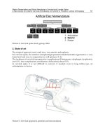
2. Biomechanics of brace action used for conservative treatment in spinal
deformity
The brace as a mean of spinal deformity conservative treatment should be based on the
following general principles:
1. Prevention of asymmetric compressive forces related to passive posture
2. Reduction of the secondary muscle imbalance
3. Prevention of the lordosing reactive forces (passive posture, repeated forward bending
movements)
4. Prevention of asymmetric torsional forces from gait
5. Production of dynamic detorsional forces involving breathing mechanics. [Rigo &
Grivas 2010]
Understanding the biomechanics of brace action is most important. The brace applies

external corrective forces to the trunk with the aim to halt the curve progression or to correct

Human Musculoskeletal Biomechanics

30
it during growth, [The Scoliosis Research Society Brace Manual, Rigo et al. 2006, Grivas et al.
2003, 2010, Negrini et al.2010a] or to avoid further progression of an already established
pathological curve in adulthood.
To achieve these goals, rigid supports or elastic bands can be used [Coillard et al. 2003,
Wong et al 2008] and braces can be custom-made or prefabricated [Weiss et al 2008, Sankar
et al 2007, Wong et 2005a, 2005b].
The spinal correction is accomplished by the application of mechanical forces with the
intention to reduce the pathological compression on given parts of the vertebral column
(usually the concave side), while increasing it on others, (usually the convex side). This will
result in a more symmetrical and natural loading and will make possible proper spinal
growth [Lupparelli et al. 2002, Castro 2003, Weiss & Hawes 2004]. It will also prevent
progressive degeneration of the spine [Lupparelli et al. 2002, Stokes et al 2006, Stokes 2008].
Although this is an old concept, the theory has been reinforced over time and for IS was
recently summarized in the “vicious cycle” hypothesis [Stokes et al 2006], where it is
proposed that lateral spinal curvature produces asymmetrical loading of the skeletally
immature spine through movement and neuromuscular control, which in turn causes
asymmetrical growth and hence progressive wedging deformity. In this respect, the role of
the intervertebral discs in the progression of IS and in its possible correction using bracing
has also recently been considered [Grivas et al 2006 Grivas et al 2008a]. Conversely, bracing
could establish a useful “virtuous cycle”, and as a result could lead to gradual reduction of
the asymmetry present in scoliosis [Rigo et al 2006, Rigo et al 2008]. In accordance with these
theories, a novel concept describing a comprehensive model of IS progression, based on the
patho-biomechanics of the deforming “three joint complex” was also recently presented
[Grivas et al 2009].
An alternative hypothesis suggests that the use of braces leads to neuro-motor

reorganization caused by the changes in external and proprioceptive inputs and movement
resulting from the constraint of bracing [Coillard et al 2002, Odermattet al 2003, Negrini et al
2006, Smania et al 2008]. According to this hypothesis, braces are considered the drivers of
movement while they increase external and internal bodily sensations. This permanently
changes motor behaviours, even when the brace is removed, and can have a long-term effect
on bone formation. This hypothesis can be easily applied also at all pathologies and ages;
can be considered correct in terms of trunk behaviour and neuro-muscular organization,
while its possible effect on growing bone needs further investigation. Two other interesting
and significant concepts to explain the actions of the brace have been discussed. One
suggests that the brace provides mechanical support to the body (passive component), while
the other suggests that the patient pulls his/her body away from pressure sites (active
component) to correct the curve. Such divergent theories illustrate the complexity of this
problem, but the most important point of brace treatment is to provide the three
dimensional correction of the spinal deformity, and methodologies must be developed with
this in mind [Negrini & Grivas 2010, Bagnall et 2009].
3. Treatment management principles and outcome description
The analysis of the treatment management principles and outcome description is beyond the
scope of this chapter, which describes the European braces in use. However it was
considered that it would be very useful to cite them, at least epigrammatically and give to
the reader the existing useful references.