Hydrodynamics Natural Water Bodies Part 3 potx
Bạn đang xem bản rút gọn của tài liệu. Xem và tải ngay bản đầy đủ của tài liệu tại đây (2.5 MB, 25 trang )
Hydrodynamic Control of Plankton Spatial and
Temporal Heterogeneity in Subtropical Shallow Lakes
37
95% Confidence
Interval
Calculated vs. Observed Values
Dependent variable: Turbidity
Observed Values
Calculated Values Calculated Values
Calculated vs. Observed Values
Dependent variable: Suspended Solids
Observed Values
95% Confidence
Interval
Fig. 6. Comparison between observed and calculated values for turbidity and suspended
solids through multiple regression model using the three monitoring station along the
Itapeva Lake.
3.2 Lake Mangueira
The simulated and observed values of water levels at two stations of Lake Mangueira
during the calibration and validation period are shown in Fig. 7. An independent validation
data set showed a good fit to the hydrodynamic module (R
2
≥ 0.92). The model was able to
reproduce the water level well in both extremities of Lake Mangueira. Wind-induced
currents can be considered the dominant factor controlling transport of substances and
phytoplankton in Lake Mangueira, producing advective movement of superficial water
masses in a downwind direction. For instance, a southwest wind, with magnitude
approximately greater than 4ms
−1
, can causes a significant transport of water mass and
substances from south to north of Lake Mangueira, leading to a almost instantaneous
increase of the water level in the northeastern parts and, hence the decrease of water level in
southwestern areas (Fig. 7).
Our model results showed two characteristic water motions in the lake: oscillatory (seiche)
and circulatory. Lake Mangueira is particularly prone to wind-caused seiches because of its
shallowness, length (ca. 90 km), and width (ca. 12 km). These peculiar morphological
features lead to significant seiches of up to 1 m between the south and north ends, caused by
moderate-intensity winds blowing constantly along the longitudinal axis of the lake (NE-
SW). Depending on factors such as fetch length and the intensity and duration of the wind,
areas dominated by downwelling and upwelling can be identified (Fig. 8). For instance, if
northeast winds last longer than about 6 h, the surface water moves toward the south shore,
where the water piles up and sinks. Subsequently a longitudinal pressure gradient is formed
and produces a strong flow in the deepest layers (below 3 m) toward the north shore, where
surface waters are replaced by water that wells up from below. Such horizontal and vertical
circulatory water motions may develop if wind conditions remain stable for a day or longer.
The model was also used to determine the spatial distribution of chlorophyll-a and to
identify locations with higher growth and phytoplankton biomass in Lake Mangueira. Fig. 9
shows the spatial distribution of the phytoplankton biomass for different times during the
simulation period.
Specifically, in Lake Mangueira there is a strong gradient of phytoplankton productivity
from the littoral to pelagic zones (Fig. 9). Moreover, the model outcome suggests that there
Hydrodynamics – Natural Water Bodies
38
is a significant transport of phytoplankton and nutrients from the littoral to the pelagic
zones through hydrodynamic processes. This transport was intensified by several large
sandbank formations that are formed perpendicularly to the shoreline of the lake, carrying
nutrients and phytoplankton from the shallow to deeper areas.
wind (m/s)
wind (m/s)
Water level (m)
Water level (m)
Water level (m)
Water level (m)
― North - Obs ―•― North - Cal
― North - Obs ―•― North - Cal
― South - Obs ―•― South - Cal ― South - Obs ―•― South - Cal
Fig. 7. Time series of wind velocity and direction on Lake Mangueira, and water levels fitted
for the North and South parts of Lake Mangueira into the calibration and validation periods
(solid line - observed, dotted line - calculated). Source: Fragoso Jr. et al. (2008).
Hydrodynamic Control of Plankton Spatial and
Temporal Heterogeneity in Subtropical Shallow Lakes
39
Vector scale
(m/s)
0.1
1.81 m/s
1.78 m/s
Jan/2001 Apr/2001
Jul/2001 Sep/2001
Vector scale
(m/s)
0.1
J
an/2001
Apr/2001
Sep/2001
J
ul/2001
1.81 m/s
1.78 m/s
Fig. 8. Simulated instantaneous currents in the surface (black arrows) and bottom (gray
arrows) layers of Lake Mangueira at four different instants. A wind sleeve (circle), in each
frame, indicates the instantaneous direction and the intensity of the wind. Source: Fragoso
Jr. et al. (2011).
In addition, it was possible to identify zones with the highest productivity. There is a trend
of phytoplankton aggregation in the southwest and northeast areas, as the prevailing wind
directions coincide with the longitudinal axis of Lake Mangueira. The clear water in the
Taim wetland north of Lake Mangueira was caused by shading of emergent macrophytes,
modeled as a fixed reduction of PAR.
After 1,200 hours of simulation (50 days), the daily balance between the total primary
production and loss was negative. That means that daily losses such as respiration, excretion
and grazing by zooplankton exceeded the primary production in the photoperiod, leading to a
significant reduction of the chlorophyll-a concentration for the whole system (Fig. 9d; 9e).
We verified the modeled spatial distribution of chlorophyll-a with the distribution estimated
by remote sensing (Fig. 10). The simulated patterns had a reasonably good similarity to the
Hydrodynamics – Natural Water Bodies
40
patterns estimated from the remote-sensing data (Fig. 10a, b). In both figures, large
phytoplankton aggregations can be observed in both the southern and northern parts of
Lake Mangueira, as well as in the littoral zones.
Fig. 9. Phytoplankton dry weight concentration fields in μg l
-1
, for the whole system at
different times: (a) 14 days; (b) 28 days; (c) 43 days; (d) 57 days; (e) 71 days; and (f) 86 days.
The color bar indicates the phytoplankton biomass values. A wind sock in each frame
indicates the direction and intensity of the wind. The border between the Taim wetland and
Lake Mangueira is shown as well.
Hydrodynamic Control of Plankton Spatial and
Temporal Heterogeneity in Subtropical Shallow Lakes
41
Unfortunately we did not have independent data for phytoplankton in the simulation
period. Therefore we could only compare the median values of simulated and observed
chlorophyll-a, total nitrogen and total phosphorus for three points in Lake Mangueira,
assuming that the median values were comparable between the years. The fit of these
variables was reasonable, considering that we did not calibrate the biological parameters of
the phytoplankton module (see results in Fragoso Jr. et al., 2008). The lack of spatially and
temporally distributed data for Lake Mangueira made it impossible to compare simulated
and observed values in detail. However, the good fit in the median values of nutrients and
phytoplankton indicated that the model is a promising step toward a management tool for
subtropical ecosystems.
Fig. 10. Lake Mangueira: (a) MODIS-derived chlorophyll-a image with 1-km spatial
resolution, taken on February 8, 2003; and (b) simulated chlorophyll-a concentration for the
same date.
3.3 Hydrodynamic versus plankton
Hydrodynamic processes and biological changes occurred over different spatial and
temporal scales in these two large and long subtropical lakes. Itapeva Lake (31 km long) is
almost one-third the size of Lake Mangueira (90 km long), and therefore the hydrodynamic
response is faster in Itapeva Lake. On a time scale of hours, we can see the water movement
from one end of the lake to the other (e.g., from N to S during a NE wind and in the opposite
direction during a SW wind). Because of this rapid response, the plankton communities
showed correspondingly rapid changes in composition and abundance, especially the
phytoplankton when the resources (light and nutrients) responded promptly to wind action.
This interaction between wind on a daily scale (hours) and the shape of Itapeva Lake was a
determining factor for the observed fluctuations in the rates of change for phytoplankton
(Cardoso & Motta Marques, 2003) as well as for the spatial distribution of plankton
Hydrodynamics – Natural Water Bodies
42
communities (Cardoso & Motta Marques, 2004a, 2004b, 2004c). The rate of change in the
phytoplankton was very high, indicating the occurrence of intense, rapid environmental
changes, mainly in spring.
Marked changes in the spatial and temporal gradients of the plankton communities
occurred during the seasons of the year, in response to resuspension events induced by the
wind (Cardoso & Motta Marques, 2009). These responses were most intense precisely at the
sites where the fetch was longest. The increase in changes occurred as the result of
population replacements in the plankton communities. Resuspension renders diatoms and
protists dominant in the system, and they are replaced by cyanobacteria and rotifers when
the water becomes calm again (Cardoso & Motta Marques, 2003, 2004a, 2004b). Thus,
diatoms and protists were the general
indicator groups for lake hydrodynamic, with fast
responses in their spatial distribution. Wind-induced water dynamics acted directly on the
plankton community, resuspending species with a benthic habit.
In Itapeva Lake, water level and water velocity induced short-term spatial gradients, while
wind action (affecting turbidity, suspended solids, and water level) was most strongly
correlated with the seasonal spatial gradient (Cardoso & Motta Marques, 2009). In Lake
Mangueira, water level was most strongly correlated with the seasonal spatial gradient,
while wind action (affecting turbidity, suspended solids, and nutrients) induced spatial
gradients.
The Canonical Correspondence Analysis (CCA) suggested that some aspects of plankton
dynamics in Itapeva Lake are linked to suspended matter, which in turn is associated with
the wind-driven hydrodynamics (Cardoso & Motta Marques, 2009). Short-term patterns
could be statistically demonstrated using CCA to confirm the initial hypothesis. The link
between hydrodynamics and the plankton community in Itapeva Lake was revealed using
the appropriate spatial and temporal sampling scales. As suggested by our results, the
central premise is that different hydrodynamic processes and biological responses may
occur at different spatial and temporal scales. A rapid response of the plankton community
to wind-driven hydrodynamics was recorded by means of the sampling scheme used here,
which took into account combinations of spatial scales (horizontal) and time scale (hours).
In both lakes, the central zone of the lake takes on intermediate conditions, sometimes closer
to the North part and sometimes closer to the South, depending on the duration, direction
and velocity of the wind. This effect is very important for the horizontal gradients
evaluated, in relation to the physical and chemical water conditions as well as to the
plankton communities. In Lake Mangueira, the South zone is characterized by high water
transparency whereas the North zone is more turbid, because the latter is adjacent to the
wetland and is influenced by substances originated from the aquatic macrophyte
decomposition. In Itapeva Lake it was not possible to distinguish such clear spatial
differences. The spatial variation is directly related to wind action, because the lake is
smaller and shallower than Lake Mangueira. In addition, the prevailing NE winds and the
influence of the Três Forquilhas River on Itapeva Lake make the central zone often similar to
the South part. The high turbidity in Itapeva Lake is an important factor affecting the
composition and distribution of the plankton communities. However, in Lake Mangueira
the marked spatial differences between the North and South zones were important for the
composition and distribution of the plankton, and the influence of the wind was more
evident in the Center zone than in the two ends of the lake.
In Lake Mangueira, wind-driven hydrodynamics creates zones with particular water
dynamics (Fragoso Jr. et al., 2008). The velocity and direction of currents and water level
Hydrodynamic Control of Plankton Spatial and
Temporal Heterogeneity in Subtropical Shallow Lakes
43
changed quickly. Depending on factors such as fetch and wind, areas dominated by
downwelling and upwelling could be identified in the deepest parts. We observed a
significant horizontal spatial heterogeneity of phytoplankton associated with hydrodynamic
patterns from the south to the north shore (littoral-pelagic-littoral zones) over the winter
and summer periods. Our results suggest that there are significant horizontal gradients in
many variables
during the entire year. In general, the simulated depth-averaged
chlorophyll-a concentration increased from the pelagic to the littoral zones. This indicated
that a higher zooplankton biomass can exist in the littoral zones, leading, eventually, to
stronger top-down control on the phytoplankton in this part of the lake.
Moreover, as expected for a wind-exposed shallow lake, Lake Mangueira did not show
marked vertical gradients. The field campaigns showed that the lake is practically
unstratified, emphasizing the shallowness and vertical mixing caused by the wind-driven
hydrodynamics. This complete vertical mixing, as expected, was noted for both the pelagic
and littoral zones. However, we are still of the opinion that incorporation of horizontal
spatially explicit processes associated with the hydrodynamics is essential to understand the
dynamics of a large shallow lake. The occurrence of hydrodynamic phenomena such as the
seiches between the extreme ends, in a very long and narrow lake, is important, since
seiches function as a conveyor belt, accounting for the vertical mixing and transportation of
materials between the two ends of the lake and between the wetlands in the North and
South areas in Lake Mangueira. Seiches was very important to explain much of the spatial
changes in Itapeva Lake.
4. Conclusion
Recognition of the importance of spatial and temporal scales is a relatively recent issue in
ecological research on aquatic food webs (Bertolo et al., 1999; Woodward & Hildrew, 2002;
Bell et al., 2003; Mehner et al., 2005). Among other things, the observational or analytical
resolution necessary for identifying spatial and temporal heterogeneity in the distributions
of populations is an important issue (Dungan et al., 2002). Most ecological systems exhibit
heterogeneity and patchiness over a broad range of scales, and this patchiness is
fundamental to population dynamics, community organization and stability. Therefore,
ecological investigations require an explicit determination of spatial scales (Levin, 1992;
Hölker & Breckling, 2002), and it is essential to incorporate spatial heterogeneity into
ecological models to improve understanding of ecological processes and patterns (Hastings,
1990; Jørgensen et al., 2008).
Water movement in aquatic systems is a key factor which drives resources distribution,
resuspend and carries particles, reshape the physical habitat and makes available previously
unavailable resources. As such processes, and communities change along and patterns are
created in time and space. Ecological models incorporating hydrodynamics and trophic
structure are poised to serve as thinking pads allowing discovering and understanding
patterns in different time and space scales of aquatic ecosystems. In lake ecosystem
simulations, the horizontal spatial heterogeneity of the phytoplankton and the
hydrodynamic processes are often neglected. Our simulations showed that it is important to
consider this spatial heterogeneity in large lakes, as the water quality, community structures
and hydrodynamics are expected to differ significantly between the littoral and the pelagic
zones, and between differently shaped lakes. Especially for prediction of the water quality
(including the variability due to wind) in the littoral zones of a large lake, the incorporation
Hydrodynamics – Natural Water Bodies
44
of spatially explicit processes that are governed by hydrodynamics is essential. Such
information may be also important for lake users and for lake managers.
5. Acknowledgment
We are grateful to the Brazilian agencies FAPERGS (Fundação de Amparo à Pesquisa do
Estado do Rio Grande do Sul) and CNPq (Conselho Nacional de Pesquisa) / PELD
(Programa de Ecologia de Longa Duração) for grants in support of the authors.
6. References
APHA (American Public Health Association). (1992). Standard Methods for Examination of
Water and Wastewater
(18. ed.), APHA, ISBN-10 0875532071, ISBN-13 978-
0875532073, Washington.
Bell, T.; Neill, W.E. & Schluter, D. (2003). The effect of temporal scale on the outcome of
trophic cascade experiments.
Oecologia, Vol.134, pp. 578-586, ISSN Print 0029-8549,
ISSN Online 1432-1939.
Bertolo, A.; Lacroix, G. & Lescher-Moutoue, F. (1999). Scaling food chains in aquatic
mesocosms: do the effects of depth override the effects of planktivory?
Oecologia,
Vol.121, pp. 55-65, ISSN Print 0029-8549, ISSN Online 1432-1939.
Bonnet, M.P. & Wessen, K. (2001). ELMO, a 3-D water quality model for nutrients and
chlorophyll: first application on a lacustrine ecosystem.
Ecological Modelling,
Vol.141, pp. 19-33, ISSN 0304-3800.
Borche, A. (1996).
IPH-A Aplicativo para modelação de estuários e lagoas. Manual de utilização do
sistema.
UFRGS, Porto Alegre, Brazil.
Blumberg, A. F. & Mellor, G. L. (1987). A description of a three-dimensional coastal ocean
circulation model, In:
Three-Dimensional Coastal Ocean Models, N. S. Heaps (Ed.), 1-
16, American Geophysical Union (AGU), ISBN 0875902537, Washington, DC.
Cardoso, L. de S. & Motta Marques, D.M.L. (2003). Rate of change of the phytoplankton
community in Itapeva Lake (North Coast of Rio Grande do Sul, Brazil), based on
the wind driven hydrodynamic regime.
Hydrobiologia, Vol.497, pp. 1–12, ISSN Print
0018-8158, ISSN Online 1573-5117.
Cardoso, L. de S. & Motta Marques, D.M.L. (2004a). Seasonal composition of the
phytoplankton community in Itapeva Lake (North Coast of Rio Grande do Sul -
Brazil) in function of hydrodynamic aspects.
Acta Limnologica Brasiliensia, Vol.16,
pp. 401–416, ISSN 0102-6712.
Cardoso, L. de S. & Motta Marques, D.M.L. (2004b). Structure of the zooplankton
community in a subtropical shallow lake (Itapeva Lake - South of Brazil) and its
relationship to hydrodynamic aspects.
Hydrobiologia, Vol.518, pp. 123-134, ISSN
Print 0018-8158, ISSN Online 1573-5117.
Cardoso, L. de S. & Motta Marques, D.M.L. (2004c). The influence of hydrodynamics on the
spatial and temporal variation of phytoplankton pigments in a large, subtropical
coastal lake (Brazil).
Arquivos de Biologia e Tecnologia, Vol.47, pp. 587–600, ISSN
1516-8913.
Cardoso, L. de S. & Motta Marques, D.M.L. (2009). Hydrodynamics-driven plankton
community in a shallow lake.
Aquatic Ecology, Vol.43, pp. 73–84, ISSN Print 1386-
2588, ISSN Online 1573-5125.
Hydrodynamic Control of Plankton Spatial and
Temporal Heterogeneity in Subtropical Shallow Lakes
45
Cardoso, L. de S.; Silveira, A.L.L. & Motta Marques, D.M.L. (2003). A ação do vento como
gestor da hidrodinâmica na lagoa Itapeva (litoral norte do Rio Grande do Sul-
Brasil).
Revista Brasileira de Recursos Hídricos, Vol.8, pp. 5-15, ISSN 1807-1929.
Carrick, H.J.; Aldridge, F.J. & Schelske, C.L. (1993). Wind Influences Phytoplankton Biomass
and Composition in a Shallow, Productive Lake.
Limnology and Oceanography,
Vol.38, pp. 1179-1192, ISSN 0024-3590.
Casulli, V. (1990). Semi-Implicit Finite-Difference Methods for the 2-Dimensional Shallow-
Water Equations.
Journal of Computational Physics, Vol.86, pp. 56-74, ISSN 0021-9991.
Casulli, V. & Cattani, E. (1994). Stability, Accuracy and Efficiency of a Semiimplicit Method
for 3-Dimensional Shallow-Water Flow.
Computers & Mathematics with Applications,
Vol. 7, pp. 99-112, ISSN 0898-1221.
Casulli, V. & Cheng, R.T. (1990). Stability Analysis of Eulerian-Lagrangian Methods for the
One-Dimensional Shallow-Water Equations.
Applied Mathematical Modelling, Vol.14,
pp. 122-131, ISSN 0307-904X.
Chapra, S.C. (1997).
Surface water-quality modeling. McGraw-Hill series in water resources
and environmental engineering, ISBN 9780070113640, Boston.
Chow, V.T. (1959).
Open Channel Hydraulics, McGraw-Hill, ISBN 0073397873, New York.
Crossetti, L.; Cardoso, L. de S.; Callegaro, V.L.M.; Silva, S.A.; Werner, V.; Rosa, Z. & Motta
Marques, D.M.L. (2007). Influence of the hydrological changes on the
phytoplankton structure and dynamics in a subtropical wetland-lake system.
Acta
Limnologica Brasiliensia
, Vol.19, pp. 315–329, ISSN 0102-6712.
Dungan, J.L.; Perry, J.N.; Dale, M.R.T.; Legendre, P.; Citron-Pousty, S.; Fortin, M.J.;
Jakomulska, A.; Miriti, M. & Rosenberg, M.S. (2002). A balanced view of scale in
spatial statistical analysis.
Ecography, Vol.25, pp. 626-640, ISSN 0906-7590.
Ecoplan Engenharia Ltda (1997).
Avaliação da disponibilidade hídrica superficial e subterrânea do
litoral norte do Rio Grande do Sul, englobando todos os corpos hídricos que drenam o Rio
Tramandai
. Porto Alegre, Brazil.
Edmondson, W.T. & Lehman, J.T. (1981). The Effect of Changes in the Nutrient Income on
the Condition of Lake Washington.
Limnology and Oceanography, Vol.26, pp. 1-29,
ISSN 0024-3590.
Edwards, A.M. & Brindley, J. (1999). Zooplankton mortality and the dynamical behaviour of
plankton population models.
Bulletin of Mathematical Biology, Vol.61, pp. 303-339,
ISSN Print 0092-8240, ISSN Online 1522-9602.
Eppley, R.W. (1972). Temperature and Phytoplankton Growth in the Sea.
Fishery Bulletin
(Wash DC), Vol.70, pp. 1063-1085, ISSN 0090-0656.
Fasham, M.J.R.; Flynn, K.J.; Pondaven, P.; Anderson, T.R. & Boyd, P.W. (2006). Development
of a robust marine ecosystem model to predict the role of iron in biogeochemical
cycles: A comparison of results for iron-replete and iron-limited areas, and the
SOIREE iron-enrichment experiment.
Deep-Sea Research Part I-Oceanographic
Research Papers
, Vol. 53, pp.333-366, ISSN 0967-0637.
Fragoso Jr, C.R.; Motta Marques, D.M.L. , Collischonn, W.; Tucci, C.E.M. & Nes, E.H.V.
(2008). Modelling spatial heterogeneity of phytoplankton in Lake Mangueira, a
large shallow lake in South Brazil.
Ecological Modelling, Vol.219, pp. 125-137, ISSN
0304-3800.
Fragoso Jr., C.R.; van Nes, E.H.; Janse, J.H. & Motta Marques, D.M.L. (2009). IPH-TRIM3D-
PCLake: A three-dimensional complex dynamic model for subtropical aquatic
Hydrodynamics – Natural Water Bodies
46
ecosystems. Environmental Modelling & Software, Vol.24, pp. 1347–1348, ISSN 1364-
8152.
Fragoso Jr, C.R.; Motta Marques, D.M.L. ; Ferreira, T.F. ; Janse, J.H. ; van Nes, E.H. (2011).
Potential effects of climate change and eutrophication on a large subtropical
shallow lake. Environmental Modelling & Software, Vol. 26, pp. 1337-1348, ISSN
1364-8152.
Garcia, A.M.; Hoeinghaus, D.J.; Vieira, J.P.; Winemiller, K.O.; Marques, D. & Bemvenuti,
M.A. (2006). Preliminary examination of food web structure of Nicola Lake (Taim
Hydrological System, south Brazil) using dual C and N stable isotope analyses.
Neotropical Ichthyology, Vol.4, pp. 279-284, ISSN 1679-6225.
Gross, E.S.; Koseff, J.R. & Monismith, S.G. (1999a). Evaluation of advective schemes for
estuarine salinity simulations.
Journal of Hydraulic Engineering-Asce, Vol.125, pp. 32-
46, ISSN Print 0733-9429, ISSN Online 1943-7900.
Gross, E.S.; Koseff, J.R. & Monismith, S.G. (1999b). Three-dimensional salinity simulations of
south San Francisco Bay.
Journal of Hydraulic Engineering-Asce, Vol.125, pp. 1199-
1209, ISSN Print 0733-9429, ISSN Online 1943-7900.
Håkanson, L. (1981).
A Manual of Lake Morphometry. Springer-Verlag, ISBN-10 3540104801,
ISBN-13 978-3540104803, Berlin.
Hamilton, D.; Schladow, S. & Zic, I. (1995a).
Modelling artificial destratification of prospect and
nepean reservoirs: final report
, Centre for Water Research, University of Western
Australia.
Hamilton, D.P.; Hocking, G.C. & Patterson, J.C. (1995b). Criteria for selection of spatial
dimensionality in the application of one and two dimensional water quality
models.
Proceedings of International Congress on Modelling and Simulation, ISBN
0725908955, The University of Newcastle, Australia, june/2005.
Hastings, A. (1990). Spatial heterogeneity and ecological models.
Ecology, Vol.71, pp. 426-
428, ISSN 0012-9658.
Hölker, F. & Breckling, B. (2002). Scales, hierarchies and emergent properties in ecological
models: conceptual explanations. In:
Scales, hierarchies and emergent properties in
ecological models
, F. Hölker (Ed.), 7-27, Peter Lang, ISBN 3631389248, Frankfurt.
Imberger, J. & Patterson, J.C. (1990). Physical Limnology.
Advances in Applied Mechanics,
Vol.27, pp. 303-475, ISSN 00652156.
Janse, J.H. (2005).
Model studies on the eutrophication of shallow lakes and ditches, Wageningen
University, Wageningen.
Jørgensen, S.E. (1994).
Fundamentals of Ecological Modelling Developments in Environmental
Modelling
(3rd ed), Elsevier, ISBN 0080440150, Amsterdam.
Jørgensen, S.E.; Fath, B.D.; Grant, W.E.; Legovic, T. & Nielsen, S.N. (2008). New initiative for
thematic issues: An invitation.
Ecological Modelling, Vol.215, pp. 273-275, ISSN 0304-
3800.
Kamenir, Y.; Dubinsky, Z.; Alster, A. & Zohary, T. (2007). Stable patterns in size structure of
a phytoplankton species of Lake Kinneret.
Hydrobiologia, Vol.578, pp. 79-86, ISSN
Print 0018-8158, ISSN Online 1573-5117.
Levin, S.A. (1992). The problem of pattern and scale in ecology.
Ecology, Vol.73, pp. 1943-
1967, ISSN 0012-9658.
Lucas, L.V. (1997).
A numerical investigation of Coupled Hydrodynamics and phytoplankton
dynamics in shallow estuaries
, Univ. of Stanford, Stanford.
Hydrodynamic Control of Plankton Spatial and
Temporal Heterogeneity in Subtropical Shallow Lakes
47
Matveev, V.F. & Matveeva, L.K. (2005). Seasonal succession and long-term stability of a
pelagic community in a productive reservoir.
Marine and Freshwater Research,
Vol.56, pp. 1137-1149, ISSN 1323-1650.
Mehner, T.; Holker, F. & Kasprzak, P. (2005). Spatial and temporal heterogeneity of trophic
variables in a deep lake as reflected by repeated singular samplings.
Oikos, Vol.108,
pp. 401-409, ISSN Print 0030-1299, ISSN Online 1600-0706.
Mitra, A. & Flynn, K.J. (2007). Importance of interactions between food quality, quantity,
and gut transit time on consumer feeding, growth, and trophic dynamics.
American
Naturalist
, Vol.169, pp. 632-646, ISSN Print 00030147, ISSN Online 15375323.
Mitra, A.; Flynn, K.J. & Fasham, M.J.R. (2007). Accounting for grazing dynamics in nitrogen-
phytoplankton-zooplankton models.
Limnology and Oceanography, Vol.52, pp. 649-
661, ISSN 0024-3590.
Mukhopadhyay, B. & Bhattacharyya, R. (2006). Modelling phytoplankton allelopathy in a
nutrient-plankton model with spatial heterogeneity.
Ecological Modelling, Vol.198,
pp. 163-173, ISSN 0304-3800.
Olsen, P. & Willen, E. (1980). Phytoplankton Response to Sewage Reduction in Vattern, a
Large Oligotrophic Lake in Central Sweden.
Archiv fur Hydrobiologie, Vol.89, pp.
171-188, ISSN 0003-9136.
Platt, T.; Dickie, L.M. & Trites, R.W. (1970). Spatial Heterogeneity of Phytoplankton in a
near-Shore Environment.
Journal of the Fisheries Research Board of Canada, Vol.27, pp.
1453-1465, ISSN 0015-296X.
Rajar, R. & Cetina, M. (1997). Hydrodynamic and water quality modelling: An experience.
Ecological Modelling, Vol.101, pp. 195-207, ISSN 0304-3800.
Reynolds, C.S. (1999). Modelling phytoplankton dynamics and its application to lake
management.
Hydrobiologia, Vol.396, pp. 123-131, ISSN Print 0018-8158, ISSN
Online 1573-5117.
Sas, H. (1989).
Lake restoration by reduction of nutrient loading: expectations, experiences,
extrapolations
, Academia Verlag Richarz, ISBN-10 388345379X, ISBN-13 978-
3883453798, St. Augustin.
Scheffer, M. (1998).
Ecology of Shallow Lakes. Population and Community Biology, Chapman and
Hall, ISBN 0412749203, London.
Scheffer, M. & De Boer, R.J. (1995). Implications of spatial heterogeneity for the paradox of
enrichment.
Ecology, Vol.76, pp. 2270-2277, ISSN 0012-9658.
Schindler, D.W. (1975). Modelling the eutrophication process.
Journal of the Fisheries Research
Board of Canada
, Vol.32, pp. 1673-1674, ISSN 0015-296X.
Schladow, S.G. & Hamilton, D.P. (1997). Prediction of water quality in lakes and reservoirs
.2. Model calibration, sensitivity analysis and application.
Ecological Modelling,
Vol.96, pp. 111-123, ISSN 0304-3800.
Smith, R.A. (1980). The Theoretical Basis for Estimating Phytoplankton Production and
Specific Growth-Rate from Chlorophyll, Light and Temperature Data.
Ecological
Modelling
, Vol.10, pp. 243-264, ISSN 0304-3800.
Steele, J.H. (1978).
Spatial Pattern in Plankton Communities, Plenum Press, ISBN 030640057X,
New York.
Steele, J.H. & Henderson, E.W. (1992). A simple model for plankton patchiness.
Journal of
Plankton Research
, Vol.14, pp. 1397-1403, ISSN 0142-7873.
Hydrodynamics – Natural Water Bodies
48
Thoman, R.V. & Segna, J.S. (1980). Dynamic phytoplankton-phosphorus model of Lake
Ontario: ten-year verification and simulations. In:
Phosphorus management strategies
for lakes
, C. Loehr; C.S. Martin & W. Rast (Eds.), 153-190, Amr Arbor Science
Publishers, ISBN 0250403323, Michigan.
Tucci, C.E.M. (1998).
Modelos Hidrológicos. Coleção ABRH de Recursos Hídricos, UFRGS,
ISBN8570258232, Porto Alegre, Brazil.
Van den Berg, M.S.; Coops, H.; Meijer, M.L.; Scheffer, M. & Simons, J. (1998). Clear water
associated with a dense Char a vegetation in the shallow and turbid Lake
Veluwemeer, the Netherlands. In:
Structuring Role of Submerged Macrophytes in
Lakes
, E. Jeppesen; M. Søndergaard & K. Kristoffersen (Eds.), 339-352, Springer-
Verlag, ISBN 0387982841, New York.
White, F.M. (1974).
Viscous Fluid Flow, McGraw-Hill, ISBN 0070697124, New York.
Woodward, G. & Hildrew, A.G. (2002). Food web structure in riverine landscapes.
Freshwater Biology, Vol. 47, pp. 777-798, ISSN Print 0046-5070. ISSN Online 1365-
2427.
Wu, F.C.; Shen, H.W. & Chou, Y.J. (1999). Variation of roughness coefficients for
unsubmerged and submerged vegetation.
Journal of Hydraulic Engineering-Asce,
Vol.125, pp. 934-942, ISSN Print 0733-9429, ISSN Online 1943-7900.
Wu, J. (1982). Wind-Stress Coefficients over Sea-Surface from Breeze to Hurricane.
Journal of
Geophysical Research-Oceans and Atmospheres
, Vol.87, pp. 9704-9706, ISSN 0196-2256.
3
A Study Case of Hydrodynamics and Water
Quality Modelling: Coatzacoalcos River, Mexico
Franklin Torres-Bejarano, Hermilo Ramirez and Clemente Rodríguez
Mexican Petroleum Institute
Mexico
1. Introduction
The common basis of the modeling activities is the numerical solution of the momentum
and mass conservation equations in a fluid. For hydrodynamic modeling, the Navier-Stokes
equations are usually simplified according to the specific water body properties, obtaining,
for example, the shallow water equations, so called because the horizontal scale is much
larger than the vertical. Therefore, in cases where the river has a relation width-depth of 20
or more and for many common applications, variations in the vertical velocity are much less
important than the transverse and longitudinal direction (Gordon et al., 2004). In this sense,
the equations can be averaged to obtain the vertical approach in two dimensions in the
horizontal plane, which adequately describes the flow field for most of the rivers with these
characteristics.
At the same time, the contaminant transport models have evolved from simple analytical
equations based on idealized reactors to sophisticated numerical codes to study complex
multidimensional systems. Since the introduction of the classic Streeter-Phelps model in the
1920 to evaluate the Biochemical Oxygen Demand and dissolved oxygen in a steady state
current, contaminant transport and water quality models have been developed to
characterize and assist the analysis of a large number of water quality problems.
This chapter presents the numerical solution of the two-dimensional Saint-Venant and
Advection-Diffusion-Reaction equations to calculate the free surface flow and contaminant
transport, respectively. The solution of both equations is based on a second order Eulerian-
Lagrangian method. The advective terms are solved using the Lagrangian scheme, while the
Eulerian scheme is used for diffusive terms. The specific application to the Coatzacoalcos
River, Mexico is discussed, having as a main building block the water quality assessment
supported on mathematical modelling of hydrodynamics and contaminants transport. The
solution method here proposed for the two-dimensional equations, yields appropriate
results representing the river hydrodynamics and contaminant behaviour and distribution
when comparing whit field measurements.
In this work is presented the structure of a numerical model giving an overview of the
program scope, the conceptual design and the structure for each hydrodynamic, pollutants
transport and water quality modules that includes ANAITE/2D model (Torres-Bejarano and
Ramirez, 2007). The numerical solution scheme is detailed explained for both Saint-Venant
and the Advection-Diffusion-Reaction equation. To validate the model, some comparisons
were made between model results and different field measurements.
Hydrodynamics – Natural Water Bodies
50
2. The numerical model
The developed model is a scientific numerical hydrodynamic and water quality model
written in FORTRAN; the model has been named ANAITE/2D. The current version of this
model solves the Saint-Venant equations for hydrodynamics representation and the
Advection-Diffusion-Reaction (A-D-R) equation using a two-dimensional approach to
simulate the pollutants fate.
2.1 The hydrodynamic module
In order to obtain a better representation of the hydrodynamics reproduced by the ANAITE
model (Torres-Bejarano & Ramirez, 2007), this work presents the solution to change from
one-dimensional steady state approach to unsteady two-dimensional flow approximation,
solving the two-dimensional Saint-Venant equations (eqs. 1, 2 and 3); these equations
describe two-dimensional unsteady flow vertically averaged, representing the principles of
conservation of mass and momentum and are obtained from the Reynolds averaged Navier-
Stokes equations under certain simplifications (Chaudhry, 1993). These equations have a
wide applicability in the study of free surface flow. For example, the flow in open channels
with steep slopes (Salaheldin et al., 2000), flows over rough infiltrating surfaces (Wang et al.,
2002), propagation of flood waves Rivers (Ying et al., 2003), dam break flow (Mambretti et
al., 2008), among others.
h (hu) (hv)
0
tx y
(1)
22
tox
f
x
22
uuuh uu
uvgν
g
SS
txyx
xy
(2)
22
to
yfy
22
vvvh vv
uvgν gS S
txyy
xy
(3)
where:
Sf = friction slope, (·)
h = water depth, (m)
u = longitudinal velocity, x direction (m/s)
v = transversal velocity, y direction (m/s)
t = turbulent viscosity, (m
2
/s)
g = acceleration due to gravity, (m/s
2
)
In this equations system, it was assumed that the effect of the Coriolis force and tensions
due to wind at the free surface are negligible given the nature of the problems that focus this
work, although their inclusion in the numerical scheme can be done without difficulty.
2.2 The water quality module
The water quality model, adapted to the main stream of Coatzacoalcos river, simulates the
behaviour and concentration distributions for different water quality parameters. The water
quality module solves the following parameters, grouped according to the chemical
properties:
A Study Case of Hydrodynamics and Water Quality Modelling: Coatzacoalcos River, Mexico
51
Physics: Temperature, Salinity, Suspended Solids, Electric Conductivity.
Biochemical: Dissolved Oxygen (DO), Biochemical Oxygen Demand (BOD), Fecal
Coliforms (FC).
Eutrophication: Ammonia Nitrogen (NH
3
), Nitrates (NO
3
), Organic Nitrogen (N_org.),
Inorganic phosphorous (phosphate, PO
4
), organic Phosphorous (P_org.).
Metals: Cadmium, Chromium, Nickel, Lead, Vanadium, Zinc.
HAPs: Acenaphthene, Phenanthrene, Fluoranthene, Benzo(a)anthracene, Naphthalene.
The transport and transformation of the different environmental parameters was carried out
by applying the two-dimensional approach of A-D-R (eq. 4):
C
CCC C C
u v Ex Ey Γ
txyxxyy
(4)
where:
C = Concentration of any water quality parameter, (mg/L)
Ex = Coefficient of longitudinal dispersion, (m
2
/s)
Ey = Coefficient of transversal dispersion (m
2
/s)
Γc = Reaction mechanism (specified for each parameter) (m
-1
)
The reaction mechanism, Γc, is used to represent the water quality parameters, and it is
solved individually for each of them.
Fig. 1. Flow diagram of ANAITE/2D numerical model
Hydrodynamics – Natural Water Bodies
52
2.3 Numerical solutions
The Saint-Venant and A-D-R equations are numerically solved using a second order
Eulerian-Lagrangean method; a detailed explanation of the solution is presented in this
work. The method separates the equations into its two main components: advection and
diffusion, which are solved using a combination of Lagrangian and Eulerian techniques,
respectively. In this way, the entire equations are solved. Fig. 1 shows the flow diagram for
the model general solution.
2.3.1 Numerical grid
A numerical grid Staggered Cell type is used (Fig. 2). In this grid the scalars are evaluated in
the center of the cell and vector magnitudes on the edges.
U
i+1/2, j
V
i, j+1/2
C
i,j
x
y
C
i+1,j
C
i,j+1
V
i, j-1/2
U
i-1/2, j
edge
V
edge
U
Fig. 2. Notation for Staggered cell grid
2.3.2 Advection (Lagrangian method)
The advection solution uses a Lagrangian method whose interpolation/extrapolation
principle is base on the characteristics method. In the characteristics method is assigned to
each node at t
n+1
a particle that does not change its value as it moves along a characteristic
line defined by the flow. It locates its position in the previous time t
n
by the interpolation of
adjacent values of a characteristic value, in this case the Courant number, which is assigned
to node t
n+1
. For simplicity, the method is exemplified in one dimension, but is similar for
two or three dimensions (Fig. 3).
Assuming that the value of the variable at point P (φ
p
n
), can be calculated by interpolating
between the values φ
n
i-1
y φ
i
n
from the adjacent points x
0
and x
1
respectively (Rodriguez et
al., 2005).
If a particle at the point P travels at a constant velocity U will move a distance x + U Δt at
time t + Δt, so it is:
xt x u tt t x
p
xt t,, ,
(5)
if we apply the modified Gregory-Newton interpolation:
110 210
1
2
2
pp
fP fx px f pf f f f f
!
(6)
A Study Case of Hydrodynamics and Water Quality Modelling: Coatzacoalcos River, Mexico
53
n
b
ottom line
xxxx
P
O
0-1
i
-1
i
-2
i
p
i+
1
nnn
n
n
12
n
+1
px
()
x
-p
(1 )
x
t
x
t
U
Fig. 3. Notation used, shown in one-dimensional mesh
Where f(P), f
1
, f
0
y f
2
are the values at points P, x
1
, x
0
, and x
2
respectively, p is a weight
coefficient which positions the point P with respect to φ
i
n
and φ
i-1
n
. Since the polynomial is a
second-degree interpolation, the three terms of equation (6) are used. Substituting the
known values for the three points:
22 2
11
105050505
nn n n
p
ii i
ppppp
As the value at point P is required in a two dimensional grid, the solution is expressed as
shown in equation (7).
22 2 2
11
222 2
11111
222 2
11111
1 1 05 05 05 05
05 05 1 05 05 05 05
05 05 1 05 05 05 05
nn n
i aj b ij ij ij
nn n
ij ij ij
nn n
ij ij ij
pq qq qq
ppq qq qq
ppq qq qq
,,,,
,, ,
,, ,
(7)
where p and q, are the Courant numbers in x and y directions, respectively. The calculation
of the Courant numbers for u and v is as follows:
ij ij
uv
i
j
ut vt
Cp Cq
x
y
**
,,
() ; ()
(8)
where:
11 11 11 11
1
4
ij ij i j i j i j i j
u uuuuu
*
,,,,,,
(9)
11 11 11 11
1
4
ij ij i j i j i j i j
v vvvvv
*
,,,,,,
(10)
Hydrodynamics – Natural Water Bodies
54
α is coefficient of relaxation with typical values between 0 – 1. In this work 0.075 was used.
u*
i,j
and v*
i,j
are spatial velocities in x and y direction respectively.
The solution method is applied in a similar way to the advective terms presents in the
continuity (Eq. 1), momentum (Eqs. 2 and 3) and A-D-R (Eq. 4) equations;
φ = h, u, v y C, are
the advective variables, obtained by the lagrangian method in its second order
approximation.
2.3.3 The diffusion (Eulerian method)
Turbulent diffusion. The turbulent viscosity coefficient present in the Saint-Venant equations
is evaluated with a cero order model o mixing length model in two dimensions (vertically
averaged):
2
22
2
2
2 2 2.34 0.267
f
tm m
u
uvuv
llh
xyyx h
(11)
where:
ℓ
m
= mixing length
u
f
= friction velocity,
f
u
g
hS
κ = von Kármán constant
Thus, the diffusion terms in
x and y are solved respectively by the following formulas:
1111
11
n
n
i j ij ij i j ij ij ij ij
t
ii jj
u u uu u u uu
Dift_u
xx yy
,, , , , , ,,
(12)
1111
11
n
n
i j ij ij i j ij ij ij ij
t
ii jj
v v vv v v vv
Dift_v
xx yy
,, , , , , ,,
(13)
Detailed analysis of turbulence, their interpretation and mathematical treatment can be
found at Rodi, (1980), Rodríguez et al., (2005).
Longitudinal and transverse dispersion in rivers. The A-D-R equation evaluates the dispersion
process by
Ex and Ey coefficients.
In this work the longitudinal dispersion coefficient proposed by Seo and Cheong (1998) has
been implemented (Eq. 14):
1 428
0 620
.
.
5.915
ff
Ex W u
hu h u
(14)
The expression for estimating the transverse dispersion coefficient in a river is given by
(adapted from Martin and McCutcheon, 1999):
*
0.023E
y
hU (15)
A Study Case of Hydrodynamics and Water Quality Modelling: Coatzacoalcos River, Mexico
55
The 0.023 value was specifically obtained for the studied river. The dispersion terms in
equation (4) are numerically solved as follow:
1
11
1
1
11
1
n
ij ij
i j ij ij i j
ii i
n
ij ij
ij ij ij ij
jj j
Ex Ex
t
Disp_C C C C C
xx x
Ey Ey
t
CC CC
yy y
,,
,, , ,
,,
,, ,,
(16)
2.3.4 The pressure terms
This is the term that takes into account the external forces in the Saint-Venant equations, in
this case the gravitational forces. It is solved with a centered difference of depth values in
the calculation grid (Eq. 17).
11 11
22
nn
i j i j ij ij
hh hh
Pres_u g Pres_v g
xy
,, ,,
;
(17)
2.3.5 The continuity equation
Expanding the derivative and rearranging terms in equation (1), the continuity equation is
as follows:
11 11
1
22
n
i j i j ij ij
n
ij ij ij
ij
uu vv
h Advec_h t h h
xy
,, ,,
**
,,,
(18)
where:
11 11 11 11
1
4
ij i j i j i j i j
hh h h h
*
,,,,,
(19)
2.3.6 General solution for velocities
Grouping the obtained terms, the following general equations for velocities are reached:
1
ij
n
n
n
ij ox fx
u Advec_u t Dift_u - Pres_u tg S S
,
,
(20)
1
ij
n
n
n
ij oy fy
v Advec_v t Dift_v - Pres_v tg S S
,
,
(21)
The first element of the last term is the free surface slope, which multiplied by the gravity
represents the action of gravitational forces. This term can be expressed as:
000ox y
SzxSz
y
/; /
(22)
The second element of the last term represents the bottom stress, which causes a nonlinear
effect of flow delay and is calculated by the Manning formula:
Hydrodynamics – Natural Water Bodies
56
222 222
43 43
fx fy
nuuv nvuv
SS
hh
//
;
(23)
where:
S
f
= friction slope, (·)
n = Manning roughness coefficient
2.3.7 General solution for A-D-R equation
Finally, grouping term for A-D-R equation the solution is obtained with:
1n
n
n
ij C
C Advec_c t Disp_C t
,
(24)
As mentioned in section 2.2, Γc is solved individually for each parameter.
2.3.8 Stability requirements
Because a finite difference scheme is used, should be considered the linear stability criteria.
The selection of the time step and space must satisfy the condition of Courant-Friedrichs-
Lewy (CFL) for a stable solution. The CFL condition for two-dimensional Saint-Venant
equations can be written as (Bhallamudi and Chaudhry, 1992):
22
1
n
Rght
Cxy
xy
(25)
where:
R = magnitude of the resultant velocity, (m/s)
3. Study case: Coatzacoalcos River
The last stretch of the Coatzacoalcos River located in the Minatitlan-Coatzacoalcos Industrial
Park (MCIP), with about 40 km length, is part of an area of vast natural diversity, where the
high population concentration creates important environmental changes, due to pressures
arising mainly from consumption and industrial activities. Currently, insufficient
information exists for MCIP regarding hydrodynamics and water quality at the river stretch.
This is one of the most polluted rivers in Mexico and is consequently a critical area in terms
of industrial pollution.
Coatzacoalcos is a commercial and industrial port that offers the opportunity to operate a
transportation corridor for international traffic, the site is the development basis for
industrial, agricultural, forestry and commercial in this region; by the volume of cargo is
considered the third largest port in the Gulf of Mexico (Fig. 4). The area of Coatzacoalcos
river mouth has had a rapid urban and industrial growth in the last three decades. In this
area, the largest and most concentrated industrial chemical complex, petrochemical and
derivatives has been developed in Latin-America.
The importance of this industrial park, formed mainly by the Morelos petrochemical
complex, Cangrejera, Cosoloacaque and Pajaritos, is such that 98% of the petrochemicals
used throughout the country are produced there. Fig. 5 shows the industrial and
petrochemical facilities located in this area.
A Study Case of Hydrodynamics and Water Quality Modelling: Coatzacoalcos River, Mexico
57
Fig. 4. Location of Coatzacoalcos River
Fig. 5. Minatitlan-Coatzacoalcos industrial park and study zone
4. Results and discussion
We have developed a numerical model that solves the two-dimensional Saint-Venant
equations and the Advection-Diffusion-Reaction equation to study the pollutants transport.
Hydrodynamics – Natural Water Bodies
58
The model results show agreement with measurements of velocity direction and magnitude,
as well with water quality parameters. Therefore, it is considered that the developed model
can be implemented and applied to different situations for this study area and others rivers
with similar characteristics.
4.1 Model validation
For validation purpose, a sampling and measurement campaign was carried out in the
Coatzacoalcos river stretch from upstream of Minatitlan city (17º 57’ 00” N - 94º 33’ 00” W)
to its mouth in Gulf of Mexico (18º 09’ 32” N – 94º 24’ 41.33” W). The main objective was to
obtain velocities, bathymetry and water quality at 10 points of the Coatzacoalcos River (Fig.
6). The information obtained through direct measurements and chemical analysis is
primarily used for testing and numerical model validation.
Fig. 6. Measurements and sampling sites
Table 1 shows the water velocity magnitude, direction and location measured on the ten
stations. These values were compared with the model results. Fig. 7 and Fig. 8 show a
comparison between measured and calculated water velocities.
As shown in Fig. 7 and 8, the hydrodynamics numerical results correspond fairly well with
field measurements. The model results show agreement in direction and magnitude of the
measured velocity, which demonstrate that the model results are consistent and reliable to
the real river behaviour. Therefore, it is considered that the developed model can be
implemented and applied to different situations for the studied area.
Likewise, the water quality modules were validated by comparison with field
measurements, observing that the model results are consistent with these measurements
A Study Case of Hydrodynamics and Water Quality Modelling: Coatzacoalcos River, Mexico
59
and they are in the same order of magnitude. Fig. 9 shows some of the obtained results (each
point represents a measurement station and the solid line the model result).
Station Latitude Longitude
East Vel.
(cm/s)
North Vel.
(cm/s)
Resultant
(m/s)
Direction
(º)
1
17.96468 -94.5529350 -24.06 -42.34 0.49 60.39
2
17.97063 -94.4749317 4.75 23.65 0.24 78.65
3
18.01482 -94.4479867 -43.56 -8.69 0.44 11.28
4
18.06698 -94.4156000 -11.32 58.24 0.59 -79.00
5
18.08841 -94.4215717 -10.74 39.62 0.41 -74.83
6
18.1023 -94.4374683 9.38 -5.57 0.11 -30.69
7
18.1117 -94.4217833 36.78 -58.26 0.69 -57.74
8
18.12396 -94.4148883 34.06 -1.98 0.34 -3.33
9
18.13607 -94.4112700 6.62 -16.16 0.17 -67.72
10
18.16384 -94.4154150 -7.14 1.02 0.07 -8.15
Table 1. Measurements of water velocity
Fig. 7. Comparison between measured and calculated velocities for the river mouth
Hydrodynamics – Natural Water Bodies
60
Fig. 8. Comparison between measured and calculated velocities for the river middle part
Fig. 9. Concentration profiles for measured and calculated DO, BOD and Vanadium
A Study Case of Hydrodynamics and Water Quality Modelling: Coatzacoalcos River, Mexico
61
4.2 Numerical modeling
The initial step in the methodology implemented was the numerical grid generation, using
specialized software. Initial and boundary conditions (tide, the level of free water surface, and
hydrodynamic condition) were imposed; the model was set up with information gathered in
the measurement campaigns, as well as water balances to determine the river dynamics.
The mesh or numerical grid was created using the program ARGUS ONE
(), Fig. 10 shows the calculation grid system for Coatzacoalcos
river stretch, which has a length of about 25 km, spacing of Δx = Δy = 100 m. The grid has
163 element in the X direction and 211 points in Y direction, giving a total of 34393 elements.
Fig. 10. Grid configuration
Two simulation scenarios were performed representing dry season and rain season. The
input data required are shown in Table 2: Manning roughness coefficient, hydrological flow,
cross-sectional area, flow velocity and direction.
Parameter Dry season Rain season
Flow rate (m
3
/s)
405 1104.9
Cross section (m
2
)
812.4 2216.7
Flow velocity (m/s)
0.5 0.5
Flow direction (°)
58.78° 60.39
Manning coefficient
0.025 0.025
Table 2. Initial data for simulations
4.3 Results of hydrodynamics simulations
The simulation represents 30 days corresponding to dry and rain season. The numerical
integration time or time step was, ∆t = 2.0 s. Fig. 11 shows the obtained result for resultant
velocity.