Hydrodynamics Optimizing Methods and Tools Part 11 pot
Bạn đang xem bản rút gọn của tài liệu. Xem và tải ngay bản đầy đủ của tài liệu tại đây (1.49 MB, 30 trang )
Hydrodynamics – Optimizing Methods and Tools
288
Fig. 2. WES standard spillway profile with the transition steps proposed by García & Mateos
(1995).
The crest inlet profile strongly depends on the structure discharge operation capacities.
And the flow over the structure is analyzed based in the structure inlet design to achieve a
minor impact on the structure, to reduce cavitation risks and to optimize stilling basin.
With the pressure diagrams, it is possible to compute an operation curve to optimize the
flow over the structure. In this matter, all parameters as inflow conditions, reservoir
volume, outflow discharge and the maximum discharge capacity are enrolled in the
optimization process.
As already mentioned, basically two distinct flow regimes occur on stepped spillways, as a
function of the discharge and the step geometry (Povh, 2000). In the nappe flow, the steps
act as a series of falls and the water plunges from one step to the other. Nappe flows are
representative of low discharges capacities and large steps. On the other hand, small steps
and large discharges are addressed by the skimming flow regime. This flow regime is
characterized by a main stream that skims over the steps, which are usually assumed as
forming the so called “pseudo-bottom”. In the cavities formed by the steps and the pseudo-
bottom, recirculation vortices are generated by the movement of the main flow. Perhaps the
simplest form to quantify the transition from nappe to skimming flow is to express it
through the ratio between the critical flow depth Yc and the step height Sh. Rajaratnam
(1990) suggested the occurrence of the skimming flows for Yc/Sh > 0.8. This theme was also
a matter of study of Stephenson (1991), who introduced a Drop term, D= q
2
/gSh
3
to
distinguish between both regimes: for nappe flow, D< 0.6, and for skimming flow, D > 0.6.
Chanson (2006) proposed limits for both flow regimes. He suggested, as a limit for the
nappe flow, the approximated equation
=0.89−0.4
, while the limit for the skimming
flow was given by the following approximation:
=1.2−0.325
. This short presentation
shows that this transition is still a matter of studies, and that a more general numerical tool
is desirable to overcome the difficulties of defining a priori the flow regime along a stepped
chute, (Chinnarasri & Wongwises, 2004; Chanson, 2002). Fig. 3 shows the main
characteristics of the two flow regimes mentioned here.
Analysis of Two Phase Flows on Stepped Spillways
289
Fig. 3. Flow regimes along stepped chutes: a) Nappe flow (low discharges capacities), b)
Skimming flow (large discharges capacities).
3. Mathematical aspects
3.1 Free surface flow
The most difficult part of the interface simulation procedures is perhaps to obtain a realistic
free surface flow solution. In a free surface flow, special numerical techniques are required
to keep the position of the interface between the two phases. There are many free surface
techniques available in the literature, which involve different levels of difficulties and
several procedures to obtain a solution.
In general, the numerical methods are under constant modifications, in order to improve
their results and to avoid, as best as they can, nonphysical representations. Because the
computational tool itself is under constant improvement, increasing both, the storage and
the calculation speed capacities, this situation of constant improvement of the numerical
methods is understood as a “characteristic” of this methodology of study. In this sense, the
prediction of the behavior of interfaces is one of the problems that is being “constantly
improved”, so that different “solutions” can be found in the literature.
Some of the procedures devoted “to the capture of the interface” introduce an extra term
that accounts for the “interface compression”, which acts just in the thin interface region
between the phases. Some improvements related to the stability and efficiency calculations
are described, for example, in Rusche (2002). In the present study a time step was adjusted
to impose a maximum Courant number, and the prediction of the movement of the interface
was viewed as a consequence of drag forces and mass forces acting between the phases.
More details of the numerical procedures followed in this chapter are presented in the
Section 4.
3.2 Self-aerated flow
The phenomenon of air entrainment and bubble formation is initiated by the entrapment of
air volumes at the water surface, which are then "closed into bubbles", or really entrained
into the flow. At the upstream end of usual spillways, the flow is smooth and no air
entrainment occurs, so that it is called briefly as "black water". The flow turns into the so
called "white water", or two-phase flow, only after a distance has been traversed, which may
involve several steps, (see Fig. 4). The inception point of aeration is generally defined as the
position where the boundary layer formed at the bed of the chute attains the water surface,
(Carvalho, 1997; Boes & Hager, 2003b).
The distance travelled by the water until attaining the inception point is commonly named
as “black water length”. Downstream, after a distance in which the air is transported from
Hydrodynamics – Optimizing Methods and Tools
290
the surface of the flow to the bottom of the chute (named “transition length” by Schulz &
Simões, 2011, and Simões et al., 2011), the flow attains a “uniform regime”. Fig. 1b illustrates
this uniform flow far from the inception point (in this example, it is impossible to attest for
the uniformity of the velocity profiles, but it is possible to verify that the white-water global
characteristics are maintained). The air uptake is generally described as a consequence of the
turbulent movement at the water surface.
Fig. 4. Self-aeration: inception point and the distinct boundary layers.
Fig. 5 shows two sketches of the position of the inception point, for the two geometries
considered here (only large steps in figure 5a, and transition steps in figure 5b). As can be
seen, air is captured by the water only after the boundary layer has attained the surface.
Fig. 5. Boundary layer growth and the differences of the inlet profiles used in this study. a)
With same size for all steps, b) Initial steps with smaller size.
Analysis of Two Phase Flows on Stepped Spillways
291
The black water length (position of the aeration inception point) is a matter of continuing
studies. Tombes & Chanson (2005), for example, furnished the predictive Eq. 1.
= 9.719
(
)
.
(
∗
)
.
(1)
=
.
(
)
.
(
∗
)
.
(2)
∗
=
(
)
(3)
It is based on the distance L
i
with origin at the crest of the spillway, the flow depth Y
i
,
=
(which represents the step depth per unit width), where q
w
is the discharge per
unit width, g is the gravity acceleration, is the angle between the bed of the chute and the
horizontal, S
h
is the step height and F
*
is the dimensionless discharge. Other expressions for
the location of the inception point have been proposed by several authors. See, for example,
Chanson (1994).
The air concentration distribution, downstream of the inception point, may be obtained, for
example, using a diffusion model (Arantes et al., 2010), as proposed by Chanson (2000),
which leads to Eq. 4.
=1−ℎ
´
´
(4)
C is the void fraction, tanh is the notation for hyperbolic tangent, y it is a transverse
coordinate with origin at the pseudo bottom, D′ is a dimensionless turbulent diffusivity,
K′ is an integration constant, Y
90
is the normal distance to the pseudo-bottom where C is
equal to 90%. D′ e K′ are functions of the depth-averaged air concentration, C. As can be
seen, such equations involve constants which must be obtained from measurements.
In this study, the transition between the black water and the white water is of the major
interest. That is, the simulation of the transition of the smooth surface to the turbulent
multiphase surface flow, and the calculation of the void fraction distribution along the
flow are important for the present purposes. A sketch of the mentioned region is seen in
Fig. 6.
Fig. 6. Sketch of superficial disturbances and formation of drops and bubbles around the
interface.
Hydrodynamics – Optimizing Methods and Tools
292
3.3 Two phase flow
A two phase flow is essentially composed by two continuing fluids at different phases,
which form a dispersed phase in some “superposition region”. According to the volume
fraction of the dispersed phase, the prediction of multi-phase physical processes may differ
substantially. According to Rusche (2002), the CFD methodologies for dispersed flows have
been focused on low volume fraction so far. Processes which operate with large volumes of
the dispersed fraction present additional complexities to predict momentum transfer
between the phases and turbulence.
In the self-aerated flow along a stepped spillway, the flow behaves like an air-water jet
that becomes highly turbulent after the air entrainment took place, where the flow can be
topologically classified as dispersed. To computationally represent the localization of the
interface with the dispersed phase (composed by drops and bubbles) is an extremely
difficult task. Considering the traditional procedures, the optimization of the design of
stepped structures crucially depends on the measurement of the inception point and the
void fraction distribution (Tozzi, 1992). Both are mean values (mean position and mean
distribution), obtained from long term observations. Energy aspects are obtained from
mean depths and mean velocities (Christodoulou, 1999; Peterka, 1984). But, as such
measurements are generally made in reduced models, the scaling to prototype
dimensions may introduce deviations. When considering the cavitation risks, the scaling
up questions may be more critical (Olinger & Brighetti, 2004). The main numerical
simulation advantages rely, in principle, on the lower time consumption and lower costs,
in comparison to those of the experimental measurements (Chatila & Tabbara, 2004).
However, when simulating the flow, it is necessary to generate first a stable surface,
continuous and unbroken, and then allow its disruption, generating drops, bubbles, and a
highly distorting interface. Further, this disruption must happen in a “mean position” that
coincides with the observation, and it must be possible to obtain void fraction profiles that
allow concluding about cavitation risks. As can be seen, many numerical problems are
involved in this objective.
4. Numerical aspects
4.1 Equation for the movement of fluids
The two phase flow along a stepped spillway is modeled by the averaged Navier Stokes
equations and the averaged mass conservation equation, complemented by an equation to
address fluid deformations and stresses. In this chapter the heat and mass transfers, as well
as the phase changes, were not considered.
The flows are inherently turbulent and their characteristics were investigated here using the
k-ε turbulence model and adequate wall functions for the wall boundaries.
The averaged Navier Stokes equations neglect small scale fluctuations from the two phase
model. However, if the two phase flow has small particles in the dispersed phase, it has to
be taken into account in the analysis, in order to achieve an accurate prediction of the void
fraction.
Eq. 5 represents the Navier-Stokes equations for incompressible, viscous fluids (it is
represented here in vectorial form, thus for the usual three components). It is not discretized
in this chapter, because the rules for discretization may be found in many basic texts. But it
is understood that it is important to show that the analysis considers the classic concepts in
fluid motion.
Analysis of Two Phase Flows on Stepped Spillways
293
+∇
(
)
=−∆+∇+
(5)
is the velocity, is the density, is pressure, is time, represent the shear forces and
represent the body forces. An outline of the boundary conditions applied to solve the
equations is presented in Section 3.4.
4.2 Closure problem
As known, the averaging procedures applied to the Navier Stokes equations introduce
additional terms in the transport equations, that involve correlations of the fluctuating
components. These terms require new equations, which is known as the problem of
“turbulence closure”. Based on the Boussinesq hypothesis, it is possible to express the
turbulent stresses and the turbulent fluxes as proportional to the gradient of the mean
velocities and mean concentrations or temperatures, respectively. For the two phase flow it
is still required to examine the effects of the dispersed phase on the turbulent quantities.
There is a very wide spectrum of important length and time scales in such situations. These
scales are associated with the microscopic physics of the dispersed phase in addition to the
large structures of turbulence. The complexity of such flows may still be hardly increased if
considering high compressibility and the simultaneous resolution of the large scale motion
and the flow around all the individual dispersed particles.
4.3 Two phase methods
The physical representation of the air inception point is an application which considers
the primary complex phenomena of the breakup of a liquid jet. When considering the
simulation of the jet surface, it is necessary to track it. In general, the tracking
methodologies are classified into different categories. We have, for example the Volume
Tracking Methodology where the method maintains the interface position, the fluids are
marked by the volume fraction and conserves the volume. The volume is also conserved
in the moving mesh method, but the mesh is fitted to follow the fluid interface (Rusche,
2002).
In this study an Euler-Euler methodology is applied, in which each phase is addressed as
a continuum and both phases are represented by the introduction of the phase fractions in
the conservation equations. An “interface probability” is considered, and closure methods
are adopted to account for the terms that involve transfer of momentum between the
continuous and the dispersed phases.
In general, the numerical models are able to predict the mean movement of the free surface,
but they fail to predict the details of the interface (which are important, for example, to
incorporate air). In this study the disruption of the interface was imposed, in order to verify
if it is possible to generate realistic interface behaviors and to obtain mean values of the
relevant parameters. To attain these objectives, the conservation equations were discretized
using the finite volume method, and the PISO (Pressure-Implicit with Splitting of Operators)
algorithm was adopted as the pressure-velocity coupling scheme.
Considering the Volume of Fluid Method, VOF, the fluids are marked by the volume
fraction to represent the interface and it is based on convective schemes. The volume
fraction are bounded between the values 0 and 1 (values that correspond to the two
limiting phases).
Hydrodynamics – Optimizing Methods and Tools
294
As mentioned, in this study the VOF method was used. The volume of the fluid 1 in each
element is denoted by V
1
, while the volume of fluid 2 in the same element is denoted by V
2
.
Defining α = V
1
/V, where V is the volume of the cell or element, it implies that V
2
=1-. In
this chapter, if the cell is completely filled with water, α =1, and if the cell is completely
filled with the void phase, α =0. As usual, mass conservation equation (relevant for the
mentioned volume considerations) is given by:
+∇=0 (6)
Where, is the density, is time, is velocity.
A sharp interface can be achieved in the solver activating the term to interface compression.
Eq. 7 illustrates the mass conservation equation with the additional compression term.
+∇
(
)
+∇
(
(1−)
)
=0 (7)
Where
is a velocity field suitable to compress the interface.
Literature examples show that the mathematical model for two phase flows used by
interFoam (OpenFoam® two phase flow solver), allowed to obtain appropriated solutions
when using the mentioned interface capturing methodology. For example, when simulating
the movement of bubbles in bubble columns, two types of bubble trajectories were obtained:
a helical trajectory, for bubbles larger than 2mm, and a zigzag trajectory, for smaller
bubbles. Rusche (2002) mentions the agreement of the terminal velocity of the air bubbles
with literature empirical correlations, which are also based on the bubbles diameters, with
diameters between 1 and 5 mm. Although in the present analysis the problem of isolated
bubbles is not considered, the mentioned agreement is a positive conclusion that points to
the use of this method.
4.4 Boundary conditions
In the traditional CFD methodologies, the wall boundary condition is highly depending on
the mesh size. The no-slip condition can be applied when the size near the wall is very fine.
On the other hand the slip condition is used when the near wall mesh is very coarse. Most of
the times, the use of wall functions are appropriate and it imposes a source term at the
boundary faces (Versteeg & Malalasekera, 1995).
For the inlet boundary, two conditions were adopted here. 1) An initial condition similar to
a dambreak problem, with a column of water having a predefined finite height above the
weir crest. 2) A constant water discharge having a uniform velocity profile. The water
surface elevation upstream of the spillway crest was not specified as a boundary condition
because this height is part of the numerical solution. The constant discharge (or constant
flow rate) was imposed by a “down entrance” of water into the domain.
The dam break problem has been studied by theoretical, experimental, and numerical
analysis in hydraulic engineering due to flow propagation along rivers and channels
(Chanson & Aoki, 2001). However, in this study we were interested in the shape of the
flow generated by an abrupt break of a dam gate, which then flows over the stepped
spillway. Note that, if a constant water height would be defined upstream and far from
the weir crest, only the transient related to the growing of the depth would be observed.
So, a “water column” was imposed, and the growing and decreasing of the water depth
Analysis of Two Phase Flows on Stepped Spillways
295
along the spillway was observed. The initial boundary conditions and a subsequent
moment of the flow can be visualized in Fig.7a and Fig 7b. The second moment was taken
close to the end of the flow of the phenomenon. (Physically, it corresponds to the time of
16s).
Fig. 7. Phase fraction diagram. a) Initial water column (As an initial condition for phase
fraction, InterFoam solver requires that both phases exist into the domain, at least into some
volume cells), b) Water discharge following the structure slope.
At the outlet boundary, an extrapolation of the velocities was applied. It was applied
locating the outlet of the flow far from the flow region of main interest. The local phase
fraction varies accordingly to the diagram of Fig. 7, and it was observed that it tends to
reach a more uniform characteristic at the structure toe (this was better observed for the
constant inflow condition).
When using the k- ε model, the turbulent kinetic energy and the energy dissipation rate
must be imposed at the inlet boundaries. The actual value of these two variables is not easy
to estimate. A too high turbulence level is not desirable since it would take too much time to
dissipate. In this study, as the flow has a “visual laminar” behavior at the inlet, this
condition allowed some simplifications. The closing equations originated from k-ε model
are described by Eqs. 8,9,10,11 and 12.
2
2
111
() ( )
Re Re
et
u
uu
p
u
g
D
t
Fr
(8)
1
1
Re
t
ku P
t
(9)
12
()
1
() 1
Re
t
t
CPC
u
tT
(10)
Hydrodynamics – Optimizing Methods and Tools
296
t
T
(11)
tt
CT
(12)
Although known, the above equations are presented here to stress that the present chapter
considers the classical
ad hoc approximations for turbulent flows. The k- ε constant models
are described at Table 1 in Section 6.1.2.
5. Simulation tools
As mentioned the open softwares Salome and OpenFoam® were used here for mesh
generation and CFD, respectively. A Table with the software versions applied for
simulations in this study is described at the Appendix II, as well as those respective websites
for download.
5.1 Mesh generation
To simulate the flow over the domain, a structured mesh was generated at Salome software
that is produced by OpenCascade. Some difficulties arise for the mesh generation in classical
spillways, which are associated with the shape of the crest of the inlet structure (used to
provide a sub-critical inflow condition). The structured mesh generation was a choice to
have a mesh with hexahedral elements, which are highly recommended in the literature for
treatment of free surface problems.
There are many free softwares for mesh generation available for download, therefore many
of them don´t have the ability to generate a hexahedral mesh. In this way, it must also be
mentioned that some of the aroused difficulties may be related to the limitations of the
specific software. In this case, a structured mesh was generated, based on the software
characteristics for hexahedral algorithms.
Limiting the y+ value (One of the parameters that indicate mesh refinement), it is possible
to reach more accurate results. However, the computational costs may significantly
increase.
Some general characteristics are mentioned here, as the case of adopting a too coarse grid,
which leads to the situation that the results obtained are rather independent of the
turbulence model, because the numerical diffusion dominates over the turbulent
diffusion.
As an auxiliary tool to the mesh algorithm the domain were partitioned with many
horizontals and vertical plans to direct the algorithm in the specific regions as small steps
and crest. In this way the mesh is extremely refined in these regions, as shown in Fig. 8.
The mesh used to represent the domain in this study has approximately 3,5 million of
hexahedral elements. It is a tri-dimension mesh. However the domain in the z-direction is
simulated for 1m of length and the mesh for this direction has a reduced number of eight
columns.
After generating the mesh, and creating the faces to apply the boundary conditions at
Salome software, it can be easily exported to OpenFoam® through the “.*UNV” file format.
At OpenFoam® all mesh properties can be checked and at the boundary file at the
“\case\constant\polymesh\” path the boundary condition properties for any face can be
visualized and edited.
Analysis of Two Phase Flows on Stepped Spillways
297
Fig. 8. Ilustration of structured hexahedral mesh.
6. Simulation and flow details
6.1 Setup
In this study, OpenFoam-1.7.1 were used to conduct the numerical results (as described in
Appendix II). All the numerical analyses were processed considering that the chute is
composed by a prismatic channel with rectangular cross section and having a stepped bed.
The flow calculations involved discharges varying from 0.5m
3
/s to 20m
3
/s. The discharge
condition directly influences the flow regime over the structure. This range was used to test
the performance of the program and the adopted procedures.
The inlet conditions for the gas phase fraction and the liquid velocity were taken directly
from inlet water discharge measurements found in the literature. By The maximum specific
discharge applied for a good hydraulic performance is 25-30 m
3
/s m (Boes & Minor, 2000).
The interface momentum transfer (Rusche, 2002) is used to account for the lift force and
predict the phase fraction.
The surface tension coefficient between the two phases is set with the value of 0.07N/m. The
gravitational acceleration had the value of 9.81 m/s
2
. The outlet velocity was fixed with a
zero gradient far from the interesting flow region and all walls were treated with wall
boundaries lawyers. The water properties were considered at the temperature of 298K.
The time precision was automatically adjusted by the solver. Initially it was set to have the
value of 0.0001s. Therefore with the solver feature to automatically adjust the time step, it
suffered changes trough the time to attempt the maximum Courant Number specified as a
precision acceptable to the numerical simulation.
In the phase fraction field the solver allow to set a number of sub-cycles in which the phase
fraction equation is solved without doing an extremely reduction in the time step and
hardly increasing the cost with time precision.
Hydrodynamics – Optimizing Methods and Tools
298
In the PISO algorithm, the number of correction for the pressure was set to three. To the
initial conditions group of sets, all patches defined as faces in the process of mess generation
to represent the described domain in the Salome software had a value assigned for volume
fraction, pressure and velocity respecting the interaction between them to represent the
initial physical properties of the domain described in the Section 4.4.
The divergence terms in the velocity equations and in phase fraction equations were
discretized using a central difference scheme. While for the Laplacian terms a Gauss upwind
scheme was defined. For temporal discretization a Crank-Nicolson method was used.
6.1.1 Discretization schemes
An accurate numerical scheme is very important to obtain a solution. In order to check the
influence of the numerical scheme on the solution, two different configurations for the
numerical discretization have been used. With the present model, the two phase flows are
better predicted with a higher order scheme. The first order scheme is not able to correctly
predict the flow around the spillway crest without producing very large oscillations, as
shown in Fig. 9. On the other hand, the second order schemes produce a large and stable
recirculation bubble zone between the steps (while the first order did not generate such
recirculation zone). Both schemes were used, because the main characteristics of the flow
were still being adjusted, but it is necessary to use a more adequate scheme to reproduce the
interfaces between air and water (free flow and between the steps). Due to the large size of
the domain, and the related computational costs, only some more critical regions were
refined. The numerical mesh was refined, for example, around the ogee profile, where the
oscillations were observed. The different discretization schemes and mesh refinements were
also used to check the sensibility of the model. It was observed, as expected, that not refined
discretization lead to unreal interface waves, which increase significantly. As pressure
condition in the flow, the hydrostatic pressure gradient was used. Further, most of the tests
in this study were run using an upwind scheme.
Depending on the boundary conditions applied, the flow can be always supercritical, or it
can achieve a supercritical condition inside the domain. In this case, the relevant boundary
condition is the discharge applied at the inlet, which directly influences the flow regime.
Fig. 9. The influence of the first order discretization scheme along the first part of the surface
for the flow over the spillway with varying step sizes.
Analysis of Two Phase Flows on Stepped Spillways
299
The distance covered by the subcritical flow, for the adopted inlet conditions, allowed
investigating the surface characteristics of the flow along the hydraulic structures for both
the proposed inlet profiles, as shown in Fig. 5a and Fig. 5b, and Fig. 10a and Fig. 10b,
respectively. Although in all situations a region with “unbroken liquid” is observed,
followed by the broken liquid, the calculated surface did not maintain a smooth
characteristic, although with smaller instabilities in relation to Fig. 9. As the breaking of
the interface was an objective of this study, the numerical schemes were not chosen to
guarantee the unconditional stability of the surface. However, as mentioned, they
produced instabilities from the very beginning of the accelerated region (spillway
entrance), and not only after attaining the position where the boundary layer coincides
with the surface of the liquid.
The algorithm PISO used in this study is based on the assumption that the momentum
discretization may be safely kept through a series of pressure correctors. It needs small time-
steps. As a consequence, the PISO algorithm is also sensitive to the mesh quality. Aiming to
guarantee the convergence, the Courant number, Co, must keep a low value (it is function of
the time step, the magnitude of the velocity through the element, and the element size)
(Versteeg & Malalasekera, 1995). In order to check the influence of the mesh size in the
solution, a more refined mesh can be tested.
Fig. 10. Inlet profile: a) Initial structure steps with smaller size. b) With same size for all
structure steps.
6.1.2 Turbulence properties
As mentioned, the k- averaged turbulence model was used. As expected in the RANS
computations, the simulations converged to steady solutions. Table 1 shows the values of
the constants usually adopted for the k- model (see Eq. 7 through 11).
C
µ
C
ε1
C
ε2
0.09 1.44 1.92 1.0 1.3
Table 1. Empirical constants of k-ε model.
Hydrodynamics – Optimizing Methods and Tools
300
7. Preliminary Results
7.1 Pressure diagram distribution
The pressure distributions along the steps are important to study the risk of cavitation in
stepped chutes (Franc & Michel, 2004). It is not only the position of the lower pressure that is
important, but also its value and frequency. In particular, the results calculated in the
present study show no qualitative differences between the measured literature data, when
considering the position and the mean pressure distribution analysis (Amador, 2005). As
mentioned, the frequency of the low values is important, which points to the need of
instantaneous values, and not only the mean profiles.
The negative pressure plotted in Fig. 11 were also predicted by Chen et al. (2002) for a WES
structure with the transition steps.
Fig. 11. Negative Pressure.
a) Along stepped chute, b) In a step along the structure.
The pressure distributions over the steps in a stepped chute depend on the position of the
faces of the steps. In the vertical face a separation flow region occurs and the pressure
achieve negative values. Over the horizontal face the pressure distribution is influenced by
the recirculation in the cavity, which results in a positive value for the mean pressure. The
last step of Fig. 11a, amplified in Fig. 11b, shows this difference between the behavior of the
pressure along the horizontal and vertical surfaces.
7.2 Velocity distribution
The velocity of an aerated flow is expected to be higher than the velocity of an unaerated flow,
because the entrained air reduces the wall friction (Steven & Gulliver, 2007). Fig. 12 shows a
velocity diagram obtained in the present simulations. The values obtained, though not directly
compared to the results of other sources Cain & Wood (1981), are of the same order.
Amador (2005) described results of experiments of velocity fields over steps located in the
developing flow region, were the growth of the boundary layer was analyzed (upstream of
the inception point). The study shows the presence of large size eddies at the corner of the
step faces, and recirculation areas. Recirculation and air concentration distributions were
also investigated by Matos et al. (2001). The authors mentioned differences for the flows
between the step edges and in the steps cavities, describing it and mentioning the effects of
turbulence intensity.
Analysis of Two Phase Flows on Stepped Spillways
301
In this study, a calculated velocity field is shown in Fig. 12, where the region of maximum
velocity, for example, is easy to be observed. As can be seen, the mentioned recirculation is
adequately reproduced, which corresponds to the negative horizontal velocity that can
happen between the steps.
Fig. 12. Velocity distribution along the structure.
7.3 Void fraction distribution
As described before, the attention of this chapter is more concentrated in the phenomena
related with the air transfer between the two phases interface. Fig. 13 shows an
instantaneous of the position of the interface and of the void distribution, obtained
following the present procedures. In this case, the example is for constant steps. The
imposed flow rate was 15 m
3
/s m.
Fig. 13. Skimming flow regime. Result for constant steps at the entrance.
Hydrodynamics – Optimizing Methods and Tools
302
As can be seen, the surface is highly distorted, reproducing the conditions found in real flows.
The deformations characterize entrapped air, as defined by Wilhelm & Gulliver (2005), and not
entrained air, but they also allow to calculate a mean “void concentration”, a procedure
followed to check the methodology which is being tested here. As showed by Lima et al.
(2008), measured concentration profiles may involve a relative high percentage of entrapped
air, which may induce to mistakes in the calculations of the air flow rate introduced by the
water flow. In this sense, the present methodology shows that this “entrapped air
concentration profile” may be calculated to correct the evaluation of the entrained air. In Fig.
14 the results of the present calculation of the void fraction obtained for different depths is
shown. The flow conditions are those imposed to obtain Fig. 13. As mentioned, these
simulation results show that the method allows to obtain void fraction profiles.
(a)
(b)
Fig. 14. Volumetric fraction along the flow. The position 0.0 corresponds to the bottom, and
the position 1.0 corresponds to the surface. a) Histogram of void fraction where
alpha1_average represents a statistic temporal alpha average, b) presents first results of air
entrainment at any location of the spillway, allowing the prediction of the air concentration
profiles (void fraction profiles) for all calculation domains.
Fig. 15 is an example of shown in Fig. 14b, obtained for the position indicated in Fig. 15b.
With the distribution of entrained air, the gas transfer along the flow can be estimated, or, in
Analysis of Two Phase Flows on Stepped Spillways
303
other words, the air flow discharge is obtained. This quantification is relevant, allowing to
check experimental results and predictive equations obtained from simplified models,
conducting (in a more complete stage of these studies) to a better understanding of the air
entrainment phenomena on stepped chutes. In addition, concentration fields like that shown
in Fig. 15a will allow to correlate pressure and void fraction distributions, and to recognize
regions where the air content is not enough to reduce cavitation damage (that is, the the
regions under risk of cavitation). From Peterka (1953), the air concentration that is sufficient to
avoid cavitation damage is about 5 to 8%. The inlet of air increases the mixture compressibility
and the flow becomes able to absorb the impact of collapsing vaporized bubbles.
Fig. 15a also shows the concentration regions defined by Chanson (1997), considered here to
verify the possibility of obtaining practical information of such simulations. Accordingly to
Chanson (1997), three concentration ranges can be considered in the concentration analyses,
as shown in Table 2.
Rate Classification
C < 0.3 to 0.4 Clear water comprising air bubbles
C > 0.6 to 0.7 Air flow comprising water droplets
C > 0.7 Two-phase flow with equal air and water contents
Table 2. Main regions of concentration profiles. (Chanson, 1997)
As already mentioned, two examples are considered: The opening of a dam gate, a transient
situation, and a steady-state simulation that allows evaluating changes of the void ratio
along the self-aerated spillway flow. Air concentration profiles C(y) are taken in several
cross sections at steps downstream from the inception point.
Fig. 15. Phase fraction a) Contours of isosurfaces, b) Distribution of void fraction for the 4
th
step.
8. Continuing studies
The results presented in this chapter show that the proposal of studying the breaking of the
air-water interface and the formation of a dispersed phase is a challenging issue, and is still
not definitively quantified. It was possible to show that instabilities can be produced at the
interface in a way to maintain the main flow stable, but these instabilities did not follow a
realistic behavior. The aim is to break the surface in the position of the inception point of
aeration, but the instabilities were formed in the very beginning of the accelerated region of
the flow, at the spillway entrance.
Hydrodynamics – Optimizing Methods and Tools
304
Bubbles and drops were “formed” in the numerical simulations, as shown in Fig. 16. However,
the sizes of both depend of the numerical mesh used, and, in this sense, the reproduction of
these geometrical characteristics is still limited by the mesh. In practice, smaller drops and
bubbles are formed. The numerical solution were processed with the discharge of 20 m
3
/s m.
Fig. 16. General characteristics observed in a simulated flow: 1) Unrealistic superficial
instabilities in the accelerated region of the flow; 2) Formation of drops and bubbles, as
expected; 3) Cavities between the steps.
Depending on the conditions of the flow, the abovementioned characteristics are damped,
or not observed. This is the case shown in Fig. 17, where the instabilities were minimized
and no drops or bubbles were formed along the spillway. As a conclusion, the
hydrodynamic characteristics still need to be better reproduced in the simulations, in order
to guarantee the formation of the dispersed phase. The numerical solution were processed
with the discharge of 15 m
3
/s m.
Fig. 17. Velocity distribution along the structure. In this case, no drops and bubbles are
formed.
Numerical simulations over stepped spillways which take into account the stable and
unstable regions of the interface, disrupting it and forming the dispersed phase, have not
been yet presented in the literature. However high quality measurements of different
Analysis of Two Phase Flows on Stepped Spillways
305
characteristics of such flows, including cavitation predictions, are found in the literature,
and can serve as guide for the mentioned simulations.
9. Conclusions
Skimming flow over stepped chutes were simulated to verify the possibility of obtaining
results of air entrainment in stepped spillways. The stable/unstable behavior of the air-
water interface was discussed, and the difficulties to obtain a realistic breaking of the
interface and the formation of the dispersed phase were exposed.
Two situations related to the geometry of the spillways were considered: constant step sizes
and varying step sizes. Also two situations related to the flow conditions were considered:
constant inlet water discharge, and a “sluice-gate-brake”, that is, a kind of “dam-break”
situation flowing over the stepped spillway.
Results of pressure fields, velocity fields, void fraction profiles, along the simulated
spillways were furnished, showing behaviors similar to those observed and simulated in the
literature. For the void fraction profiles, also a “entrapped air” profile was furnished,
showing that the methodology allows to confirm experimental studies about entrapped air
found in the literature.
Unrealistic behavior of the surface instabilities were observed. They were formed in the
accelerated region of the flow over the spillway, and for some flow conditions they
produced large disturbances, a negative characteristic that still need to be solved.
Drops and bubbles could be formed in the flow over the spillway, but their size was shown
to be limited by the mesh characteristics. The two fluid model adopted neglects the effects of
large scales and uses an average momentum transfer between the phases. Although the
surface deformation could be reproduced, the interface tracking calculation showed to be
difficult to apply when considering the formation of a dispersed phase.
The open codes “OpenFoam®” and “Salome” were used, showing that such codes are
capable to furnish useful results for engineers and researchers in hydraulics and fluid
mechanics.
10. APPENDIX I: Software information
The OpenFoam® software is a continuum mechanics simulation tool, but it is also an object-
oriented numerical code, and a toolkit for programming. It is written in C++ programming
language and can be freely download at the website . The CFD
library is extensive and incorporates several types of solvers. The software also contains
tools for mesh conversion from many mesh generation softwares, including commercial and
free codes. The open source code has the advantage of the “transparency”, that is, it allows
following the methodology adopted for the calculus, and the assumptions made to obtain a
solution (ever present in any code). The results also can be converted to be visualized and
post processed in a number of different softwares. A version of the Paraview software is
integrated in OpenFoam® as its standard post processing tool.
11. APPENDIX II: Useful information about the open software
Some useful links with open software information are addressed in Table 3 with the
respective version of software applied in this study.
Hydrodynamics – Optimizing Methods and Tools
306
Tools applied for numerical simulations
OpenSuSe 11.2
OpenFoam 1.7.1
ParaFoam 1.7.1
Salome 5.4
Table 3. Open software.
12. APPENDIX III: Numerical procedures in CFD software
The numerical simulations using the OpenFoam® software are basically performed by file
editing. The software is structured using three basic directories. The constant sub-
directory contains all properties folders for the fluids settings and mesh characteristics.
Some physical constants.
For InterFoam solver this directory contains three files designed as: transportProperties,
enviromentalProperties and dynamicMeshDict and a specific folder for mesh properties
named as polyMesh. Into the transportProperties all information about the properties of the
two phases can be edited. The dynamicMeshDict file allows to enable the mesh movements.
The polyMesh constant sub directory keeps all information about the mesh.
In the OpenFoam® the system sub-directory contains exactly five files: ControlDict,
DecomposeParDict, fvSchemes and setFieldsDict. The contolDict file allows users set the
simulation process information like starting, end and time step. User also can choose the
methods to save the simulation data.
In the fvSchemes system file, the descritization schemes can be setted. The fvSolution file is
responsible for all solver settings like the number of iterations.
In the free surface problems, the initial condition for the volume fraction of the two fluids
also needs to be defined. The setFieldsDict allows setting different density values for each
part of the domain. The decomposeParDict file describes the decomposition for
multiprocessing simulation.
13. Acknowledgements
The authors are indebted to the Conselho Nacional de Desenvolvimento Científico (CNPq)
and FAPESP-Fundacão de Amparo Pesquisa do Estado de São Paulo (proc. 2010/52071-0*)
for the financial support to this study.
14. References
Amador, A. (2005). Comportamiento hidráulico de los aliaderos escalonados em presas de
hormigòn compactado. Master's thesis, Universitat Politécnica de Cataluya,
Barcelona.
Arantes, E., Porto, R., Gulliver, J., Lima, A., & Schulz, H. (2010). Lower nappe aeration in
smooth channels: experimental data and numerical simulation. Anais da,
82(2):521{537}.
Arantes E.J. (2007). Caracterização do Escoamento sobre Vertedores em Degraus via CFD.
Tese de Doutorado, Escola de Engenharia, Universidade de São Paulo, São Carlos,
Brasil, 204 p.
Boes, R.M. & Hager, W.H. (2003a). “Hydraulic design of stepped spillways”. ASCE, Journal
of Hydraulic Engineering. v.129, n.9, p.671-679, Sep.
Analysis of Two Phase Flows on Stepped Spillways
307
Boes, R.M. & Hager, W.H. (2003b). “Two-Phase flow characteristics of stepped spillways.
ASCE, Journal of Hydraulic Engineering”. v.129, n.9, p.661-670.
Boes, R. M.; Minor, H. E. Guidelines for the hydraulic design of stepped spillways. Proc. Int.
Workshop on Hydraulics of Stepped Spillways, VAW, ETH, Zurich. Balkema
Rotterdam, 2000. p. 163-170.
Cain P. & I.R. Wood (1981). Measurements of self-aerated flow on a spillway. Journal of
Hydraulic Engineering, ASCE, vol. 107(11), pp. 1425-1444.
Carvalho, P.D. (1997) Aeração de Escoamentos de Alta Velocidade em Canais de Forte
Declividade; Tese de doutorado apresentada à Escola de Engenharia de São Carlos
da Universidade de São Paulo, São Carlos, S.P, 1997.
Chamani, M. R. (2000). “Air inception in skimming flow regime over stepped spillways”. In.
H. E. Minor e W. H. Hager (Ed.) International Workshop on Hydraulics of Stepped
Spillways, Zürich, Switzerland: 61-67. Balkema.
Chanson, H. (1994). Aeration and de-aeration at bottom aeration devices on spillways.
Canadian Journal of Civil Engineering, 21(3):404{409}.
Chanson, H. (1997). Air bubble entrainment in free surface turbulent shear flows. Academic
Press, page 401.
Chanson, H. (2000). Discussion of characteristics of skimming flow over stepped spillways.
Journal of hydraulic Engineering.
Chanson, H. (2001). “Hydraulic design of stepped spillways and downstream energy
dissipation”. Dam Engineering, v.11, n.4, p.205-242.
Chanson, H. (2002). The hydraulics of stepped chutes and spillways. The Netherlands: A. A.
Balkema Publishers. 384 p.
Chanson, H. (2006). Hydraulics of skimming fows on stepped chutes: The effects of infow
conditions? Journal of Hydraulic Research, 44:51{60}.
Chanson, H. & Aoki, S. (2001). "Dam Break Wave with Significant Energy Dissipation : Two
Case Studies." Proc. 29th IAHR Congress, Beijing, China, Theme C, Tsinghua
University Press, Beijing, G. LI Ed., pp. 311-318.
Chatila, J. & Tabbara, M. (2004). Computational modeling of fow over an ogee spillway.
Computers & Structures, 82:1805{1812}.
Chen, X., Dai, G. & Liu, H. (2002). Volume of fuid model for turbulence numerical
simulation of stepped flow. Journal of Hydraulic Engineering, 128(7):683{688}.
Chinnarasri, C. & Wongwises, S. (2004). “Flow regime and energy loss on chutes with upward
inclined steps”. Canadian Journal of Civil Engineering. v.31, p.870-879, Oct
Christodoulou, G. (1999). “Design of stepped spillways for optimal energy dissipation”.
Hydropower & Dams. 6(5): 90-93. X Simpósio de Recursos Hídricos do Nordeste 14.
Essery, I. & Horner, M. (1978). The hydraulic design of stepped spillways. Technical report,
CIRIA.
Franc, J. & Michel, J. (2004). Fundamentals of Cavitation (Fluid Mechanics and Its
Applications). Springer.
Frizell, K. & Melford, B. (1991). Designing spillways to prevent cavitation damage. Concrete
International, 13:58{64}.
Hager, W.H. (1991). “Uniform aerated chute flow”. Journal of Hydraulic Engineering, v.117,
n.4, p.528-533, April.
García, E. & Mateos, I. (1995). Aliviaderos escalonados. diseno de la transicion entre el
umbral y la rápida escalonada. Ingenieria Civil, 99:3323 {3341}.
Gomes, J.F. (2006). Campo de pressões: condições de incipiência à cavitação em vertedouros
em degraus com declividade 1V:0,75H. 2006. 161 f. Tese (Doutorado) – Instituto de
Pesquisas Hidráulicas, Universidade Federal do Rio Grande do Sul, Porto Alegre.
Hydrodynamics – Optimizing Methods and Tools
308
Jacobsen, F. (2009). Application of OpenFoam for designing hydraulic water structures.
Open source CFD Iternational conference.
Lima, A.C.M. (2003) Caracterização de Estrutura Turbulenta em Escoamentos Aerados em
Canal de Forte Declividade com auxílio de Velocimetria a Laser, 2003. Tese de
doutorado apresentada à Escola de Engenharia de São Carlos da Universidade de
São Paulo, São Carlos, S.P., Brasil.
Lima, A.C.M.; Schulz, H.E. & Guliver, J.S. (2008) “Air Uptake along the Lower Nappe of a
Spillway Aerator”, Journal of Hydraulic Research, v. 46, n. 6, p. 839-843.
Matos, J., Pinheiro, A. N., de Carvalho Quintela, A., and Frizell, K. H. (2001). “On the role of
stepped overlays to increase spillway capacity of embankment dams.” ICOLD
European Symposium (NNCOLD), Geiranger, Norway, 473-483.
Ohtsu I., Yasuda Y. & Takahashi, M. (2004). “Flows characteristics of skimming flows in stepped
channels”. ASCE, Journal of Hydraulic Engineering. v.130, n.9, p.860-869, Sept.
Olinger, J. C. (2001). Contribuição ao estudo da distribuição de pressões nos vertedouros em
degraus. 2001. 230 f. Tese (Doutorado) - Escola Politécnica, Universidade de São Paulo.
Olinger, J. C. & Brighetti, G. (2004). “Distribuição de Pressões em Vertedouros em Degraus”.
RBRH: Revista Brasileira de Recursos Hídricos, v.9, n.1, p.67-83, Jan/Mar
Peterka, A. J. (1953). “The effect of entrained air on cavitation pitting”. Joint Meeting Paper,
IAHR/ASCE, Minneapolis, Minnesota, Aug
Peterka, A. J. (1984). Hydraulic design of spillways and energy dissipators. A Water Resources
Technical Publication, Engineering Monograph Nº 25, United States Department of
the Interior, Bureau of Reclamation. Denver, Colorado: eight printing, May.
Posvh, P.H. (2000). Avaliação da energia residual a jusante de vertedouros em degraus com
fluxos em regime skimming flow. 2000. 142 f. Dissertação (Mestrado em
Engenharia Hidráulica) - Departamento de Tecnologia, Universidade Federal do
Paraná, Curitiba.
Rajaratnam, N. 1990. Skimming flow in stepped spillways. Journal of Hydraulic
Engineering, ASCE, 116 (4): 587-591. Discussion: 118 (1): 111-114.
Rusche, H. (2002). Computational fluid dynamics of dispersed two-phase flows at high
phase fractions. PHD Thesis, Imperial College of Science, Technology and
Medicine, UK.
Simões, A.L.A.; Schulz, H.E. & Porto, R.M. (2011) Transition length between water and air-
water flows on stepped chutes. WIT Transactions on Engineering Sciences
(Computational Methods in Multiphase Flow VI, Kos, Greece), Vol 70, pp.95-105.
Schulz, H.E. & Simões, A.L.A (2011). Desenvolvimento da superfície livre em escoamentos
aerados: analogia com leis básicas de transferência. Laboratório de Turbulência e
Reologia - LTR, Relatório I/II/11.
Stephenson, D. Energy dissipation down stepped spillways. Water Power & Dam
Construction, Sutton, v.43, n.9, p.27-30, Sept. 1991.
Tozzi, M.J. (1992). Caracterização/comportamento de escoamentos em vertedouros com
paramento em degraus. 1992. Tese (Doutorado) – Universidade de São Paulo 1992.
Toombes, L. & Chanson, H. (2005). Air entrainment and velocity redistribution in a bottom
outlet jet flow. XXXI IAHR Congress, pages 2716{ 2726}.54
Versteeg, H.K. & Malalasekera, W. (1995). An introduction to computational fuid dynamics.
The finite volume method. Longman Scientific & Technical.
Wilhelms, S.C. & Gulliver, J.S. (2005). Bubbles and Waves Description of Self-aerated
Spillway. Journal of Hydraulic Research, 43(5): 522–531.
Part 4
Hydrodynamics and Heat/Mass Transfer
14
The Influence of the Hydrodynamic Conditions
on the Performance of Membrane Distillation
Marek Gryta
West Pomeranian University of Technology, Szczecin
Poland
1. Introduction
Membrane distillation (MD) is an evaporation/condensation process of volatile
components through a hydrophobic porous membrane. The maintenance of gas phase
inside the membrane pores is a fundamental condition required to carry out the MD
process. A hydrophobic nature of the membrane prevents liquid penetration into the
pores. Membranes having these properties are prepared from polymers with a low value
of the surface energy, such as polypropylene (PP), polytetrafluoroethylene (PTFE) or
polyvinilidene fluoride (PVDF) (Alklaibi & Lior, 2005; Bonyadi & Chung, 2009, Gryta &
Barancewicz, 2010). Similar to other distillation processes also MD requires energy for
water evaporation. The hydrodynamic conditions occurring in the membrane modules
influence on the heat and mass transfers, and have a significant effect on the MD process
efficiency.
The MD separation mechanism is based on vapour/liquid equilibrium of a liquid mixture.
For solutions containing non-volatile solutes only the water vapour is transferred through
the membrane; hence, the obtained distillate comprises demineralized water (Alklaibi &
Lior, 2004; Gryta, 2005a; Schneider et al., 1988). However, when the feed contains various
volatile components, they are also transferred through the membranes to the distillate (El-
Bourawi et al., 2006; Gryta, 2010a; Gryta et al., 2006a). Based on this separation mechanism,
the major application areas of MD include water treatment technology, seawater
desalination, production of high purity water and the concentration of aqueous solutions
(El-Bourawi et al., 2006; Drioli et al., 2004, Gryta, 2006a, 2010b; Karakulski et al., 2006;
Martínez-Díez & Vázquez-González, 1999; Srisurichan et al., 2005; Teoh et al., 2008).
A few modes of MD process are known: direct contact membrane distillation (DCMD), air
gap membrane distillation (AGMD), sweeping gas membrane distillation (SGMD), vacuum
membrane distillation (VMD) and osmotic membrane distillation (OMD). These variants
differ in the manner of permeate collection, the mass transfer mechanism through the
membrane, and the reason for driving force formation (Alklaibi & Lior, 2005; Gryta, 2005a).
The most frequently studied and described mode of MD process is a DCMD variant. In this
case the surfaces of the membrane are in a direct contact with the two liquid phases, hot
feed and cold distillate (Fig. 1). The DCMD process proceeds at atmospheric pressure and at
temperatures that are much lower than the normal boiling point of the feed solutions. This
allows the utilization of solar heat or so-called waste heat, e.g. the condensate from turbines
or heat exchangers (Banat & Jwaied, 2008; Bui et al., 2010; Li & Sirkar, 2004).