Indoor and Outdoor Air Pollution Part 5 pot

Development and Evaluation of a Dispersion Model to Predict Downwind Concentrations
of Particulate Emissions from Land Application of Class B Biosolids in Unstable Conditions
31
analytical solution given by Sutton (1953) to predict the concentrations for ground level area
sources. The new model has been evaluated using the data collected in 2009 and the
regression equation given by Brooks et al. (2005) based on their field work.
3. Field sampling study
In the summer of 2009, a field study was conducted to collect particles emitted during the land
application of biosolids. Particle emissions were collected for three days during the application
(application), and for two days after the application (post-application) of biosolids. An
agricultural field, scheduled for application of Class B biosolids in Northwest Ohio was
selected for the sampling. The biosolids were applied on this field by injection method.
Particle samples were collected via the use of two GRIMM 1.108 aerosol samplers operating at
airflow of 1.2 l/minute. The gravimetric data in 16 channels over the size range 0.23 µm < d <
20 µm was collected for a total of six hours every sampling day. The samplers were placed
onto specially arranged tables raised to a height so that the intake nozzle was at average
human breathing height of 1.5 m. Two sampling stations, one station inside the field and one
outside were selected. The location of the outside sampling station at 10 m downwind from
edge of the field was changed to 20 m downwind after first three hours of sampling keeping
the location of the inside station same throughout the sampling. The monitors were reoriented
in the direction of the wind, if needed. The weather data were collected using a portable
weather station at both sampling locations inside and outside. The atmospheric parameters
defining the atmospheric stability for each hour of sampling on each sampling day are
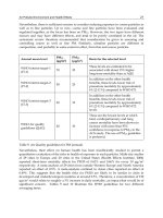
presented in Table 1. The location of outside concentration monitoring station for each hour is
also noted. The atmospheric stability for almost all sampling days was slightly unstable to
moderately unstable. On one occasion it was slightly unstable to neutral.

Date Time
Concentration
Monitor
Location from

Ed
g
e
Wind
Velocity
(m/s)
Wind
Condition
Cloud
Cover (in
tenth)
Daily Solar
Radiation
(W/m
2
)
Atmospheric
Stability
using P-G
Method*
Application
August 21,
2009
09:25–
10:25
@ 10 m
5.81
Very
High
0 755

C
10:25-
11:25
8.56 C
11:25-
12:25
8.59 C
12:25-
13:25
@ 20 m
8.93 C
13:25-
14:25
8.85 C
14:25-
15:25
8.64 C
Application
August 24,
2009
09:17–
10:17
@ 10 m
0.27
Calm 4 373
B
10:17-
11:17
0.33 B
11:17-

12:17
0.25 B
12:17-
13:17
@ 20 m 0.68 B

Indoor and Outdoor Air Pollution
32
13:17-
14:17
0.60 B
14:17-
15:17
0.41 B
Application
August 26,
2009
08:00-
09:00
@ 10 m
3.46
Low 8 288
C
9:00-
10:00
3.73 C
10:00-
11:00
2.94 C
11:00-

12:00
@ 20 m
2.27 C
12:00-
13:00
1.91 B
13:00-
14:00
2.39 C
Post-
Application
Sept. 24, 2009
08:40-
09:40
@ 10 m
0.14
Calm 8 327
B
09:40-
10:40
0.14 B
10:40-
11:40
0.25 B
11:40-
12:40
@ 20 m
0.40 B
12:40-
13:40

0.32 B
13:40-
14:40
0.13 B
Post-
Application
Sept. 25, 2009
08:30-
09:40
@ 10 m
4.07
High 5 541
C-D
09:30-
10:30
5.26 C-D
10:30-
11:30
5.87 C-D
11:30-
12:30
@ 20 m
5.45 C-D
12:30-
13:30
6.13 D
13:30-
14:30
5.78 C-D
*B: Moderately Unstable; C: Slightly Unstable; D: Neutral

Table 1. Atmospheric Conditions Observed on Each Sampling Day
The concentration data collected during the application and the post-application was
processed using Microsoft Office 2010 Excel sheets. Hourly average concentrations for each
day were calculated. Based on the average wind velocities (u) measured, sampling days
were divided into three windy conditions; low wind condition (0.5 m/s < u < 3 m/s), high
wind condition (3 m/s < u < 6 m/s), and very high wind condition (u > 6 m/s) (see Table 1).
The data collected at the inside station represented the emissions generated during the
agricultural activities. The vertical profiles of particle dispersion inside the agricultural field
during and after sludge application analyzed by Akbar et al. (2011) were used to develop a
set of emission rate equations. Hourly emission rates (Q) for each sampling day were
Development and Evaluation of a Dispersion Model to Predict Downwind Concentrations
of Particulate Emissions from Land Application of Class B Biosolids in Unstable Conditions
33
calculated using these emission rate equations. The data collected at the outside sampling
stations was used as the downwind concentration (C).
4. Model development
4.1 Shear layer model development
There are different equations available in literature for the dispersion of a ground level
release of a pollutant. However, none of the reported equations tackles the problem of wind
shear near the ground. This part focuses on deriving the analytical solution from the
convection-diffusion equation using vertical velocity profile. The following assumptions are
used in deriving the equation:
1. The wind direction is always perpendicular to the field.
2. The dispersion is of the non-fumigation type.
The velocity profile with height above the ground level is assumed to be the same for all
downwind distances. The magnitude of the wind velocity near the ground level changes
rapidly. Therefore, for the ground level discharge of the pollutant, it is very important that
the variation of the wind velocity magnitude is incorporated in the dispersion and transport
equation.
The model uses the equation for C(x,z) given by Sutton (1953):


(
,
)
=



∗
(

)
∗


(

)

∗

∗
∗exp[−

∗


((

)


∗

∗
)
] (1)
where,
C(x,z):Downwind concentration (unit/m
3
)
x: Downwind distance (m)
z: Vertical distance (m)
Q: Emission rate of pollutants (unit/sec)
u
1
: Wind velocity reference height Z
1
by the power law 
(

)
=

∗





 (2)

K
1
: Diffusivity constant reference height Z
1
given by 
(

)
=

∗





(3)
n: Exponent of power law velocity profile
m: Exponent of eddy diffusivity profile where, m = 1 – n
s: Stability parameter based on m and n ( =


)
Γ(s): Gamma function of s
The Equation (1) is integrated from x-(X/2)tox+(X/2) for a strip source with width X, and
infinite length having the origin of x ordinate at the center of the strip to obtain the
concentration from the strip. The integration gives following formulae given by Kumar and
Bhat (2008).

(

,
)
=∗




∗[


∗∗






]
(


)
(


)
(4)
where,
=() (5)
=−


∗




∗

(6)

Indoor and Outdoor Air Pollution
34
D=(,−


) (7)
=(−+2) (8)
The total concentration of the pollutant is given by following equation after considering i
number of strips in the area source.

(
,
)
=
∑
∗





∗


∗∗
























for z > 0 (9-a)


(

)
=
∑
[


(

)
∗
(

)

∗

∗ln
(


)
]













for z = 0 (9-b)
The value of x
i
is calculated using


=

+


(for i = 1) (10)
and


=

+ (for i > 1) (11)
where, x
d
is the downwind distance of monitoring station from the edge of the field.
The Equation (9-a) computes the concentration of the pollutant at chosen breathing level
while the downwind concentration at the ground is computed using Equation (9-b). These
Equations (9-a) and (9-b) were modeled into an Excel spreadsheet as the Shear Layer Model

as part of Bioaerosols Dispersion and Risk Model spreadsheet (BDRM 1.01). The
programming is done in a way so that the calculated concentrations are from the edge of the
field for different downwind distances. The development of BDRM spreadsheet is discussed
in Kumar and Bhat (2008).
5. Model evaluation
The evaluation of shear layer model involved two major steps: 1. the predicted
concentrations from the shear layer model were compared to the measured concentration
data from field study and 2. the model was evaluated using the limited data available in the
literature. In each step, the predicted data were evaluated using the calculated statistical
parameters.
5.1 Model evaluation using measured data
Multiple runs of the shear layer model were carried out to simulate characteristics of each
sampling day. Since the shear layer model was not developed for the calm conditions, only
sampling days with different windy conditions were modeled. The turbulence parameters
used to simulate the atmospheric turbulence in the shear layer model are presented in Table
2. The values of n were based on urban and rural exponents used in the air quality models
developed by the US EPA and K
1
was calculated using the equations compiled by Kumar
(1977). The predicted concentrations and the measured concentrations were formatted into a
Microsoft Excel spreadsheet to obtain average hourly concentrations. The predicted
Development and Evaluation of a Dispersion Model to Predict Downwind Concentrations
of Particulate Emissions from Land Application of Class B Biosolids in Unstable Conditions
35
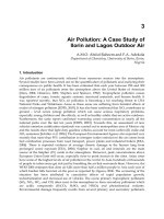
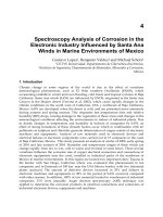
concentrations from the shear layer model were compared with the measured
concentrations (Figure 1). Visible comparison were enabled by plotting the measured vs.
predicted data on the same plot. It was found that the shear layer model over predicts the
concentration for all windy conditions except for few data points.

Model Input Neutral Unstable Stable

m
0.85 0.8 0.7
n
0.15 0.2 0.3
K
1
(m
2
/sec)
8 28.43 0.993
Table 2. Input used for the Shear Layer Model
The statistical evaluation based on the work of Hanna et al. (1993), Gudivaka and Kumar
(1990), Riswadkar and Kumar (1994) and Kumar et al. (2006), was used in this study. In
order to determine the significance of the evaluation of the model, four statistical
parameters; normalized mean square error (NMSE), fractional bias (FB), correlation
coefficient (R), and geometric mean bias (MG) were calculated.



Fig. 1. Measured vs. Predicted Concentration
The normalized mean square error (NMSE) is given by the formula,
0.00
100.00
200.00
300.00
400.00
500.00
600.00
0.00 100.00 200.00 300.00 400.00 500.00 600.00
Predicted Concentration (µg/m

3
)
Measured Concentration (µg/m
3
)
Application: Very High Wind Application: Low Wind
Post-Application: High Wind

Indoor and Outdoor Air Pollution
36

2
0
()
OP
P
CC
NMSE
CC



(12)
The fractional bias (FB) is given by the formula,

0
0
2
P
P

CC
FB
CC







(13)
The correlation coefficient (R) is given by the formula,





0
00
P
PP
CC
CCCC
r


 (14)
And the geometric mean (MG) bias is calculated by the formula,




0
exp ln ln
P
M
GCC
(15)

where, C
o
is observed values from regression equation and C
p
is predicted. These
parameters were used to further assess the predictability. The values of these statistical
parameters are presented in Table 3.

Statistical
Parameter
Complete
Dataset
Application
Post-
Application
Low Wind
Very High
Wind
High Wind
NMSE 0.17 0.31 0.017 0.21
Fractional Bias 0.23 0.41 0.09 0.21
R

0.94 0.96 0.89 0.71
MG 0.78 0.90 0.65 0.80
Table 3. Shear Layer Model Performance Using Predicted and Measured Concentrations
For a “perfect” ideal model the fractional bias and the normalized mean square error are
equal to zero. The ideal values for a geometric mean bias and the correlation coefficient
should be 1. As expected in the real life, the shear layer model is not a perfect model.
However, the acceptable range for NMSE and FB for an air quality model suggested by
Kumar et al. (1993) is given as, NMSE ≤ 0.5 and -0.5 ≤ FB ≤ 0.5. The values of NMSE and FB
for shear layer model in all wind conditions were within acceptable limits.
The geometric mean bias is a function of a logarithmic mean of the predicted and observed
data. Geometric mean bias values of 0.5-2.0 can be thought as “factor of two” over
predictions and under predictions in the mean respectively (Hanna et al., 1993). Thus the
geometric mean range for the acceptable model is given as 0.5 ≤ MG ≤ 2.0. When a data set
contains pairs of data 10 or less, then the logarithmic forms are appropriate, so that the
Development and Evaluation of a Dispersion Model to Predict Downwind Concentrations
of Particulate Emissions from Land Application of Class B Biosolids in Unstable Conditions
37
under predictions and the over predictions receive equal weight. The values of MG for each
condition are better representation of the behavior of a model to assess whether a model is
over predicting or under predicting in a particular situation. From Table 5 it was observed
that the shear layer model over predicts the concentrations under almost all the conditions.
This may be due to the factors such as the use of concentrations measured at 1.5 m as
ground level concentrations, the concept of eddy diffusivity for atmospheric turbulence in
the new model, and the assumptions made for other model inputs. It was also observed that
during the low wind conditions the predictions were closer to reality (MG=0.90) than during
other wind conditions.
5.2 Model evaluation using literature data
To evaluate the model based on the literature data, an evaluation case was developed based
on Brooks et al. (2005)

study. The paper gives a regression equation based on the data
collected downwind of the application site. For this evaluation purpose a constant emission
rate of 4.13 particles/ m
2
/sec as given in the paper was used. Wind velocity was 2.29 m/s at
10 m height. Based on the atmospheric conditions described in the literature, the slightly
stable to near neutral stability condition was assumed for the simulation. The input values
for the stability parameters used for shear layer model were used from Table 2.
The predicted concentrations were plotted along with the concentrations obtained from the
regression equation for various downwind distances (See Figure 2). The comparison of
predicted concentration with the observed concentration from regression equation was plotted
(See Figure 3). It was observed from the figures that shear layer model under predicts the
concentration for shorter downwind distance (x < 15 m) closer to the field, but for the higher
downwind distances (x > 20 m) the model over predicts the concentrations. As a result, the
shear layer model, again, was observed to over predict the downwind concentrations.




Fig. 2. Comparison of Concentrations predicted using the Shear Layer Model and
Regression Equation by Brooks et al. (2005)
0
200
400
600
800
1000
0 5 10 15 20 25 30 35 40 45 50
Concentration (µg/m

3
)
Downwind Distance (m)
Shear Layer Model Regression Equation

Indoor and Outdoor Air Pollution
38

Fig. 3. Concentration using Regression Equation vs. Predicted Concentration from the Shear
Layer Model
Again, performance measures were calculated from the modeled and the observed
concentrations. The statistical parameter NMSE, FB, correlation coefficient, and geometric
mean (MG) were calculated using the previously stated equations (See Table 4). It was
determined from these performance measures that even though the shear layer model was
not a perfect model, the parameters were within the acceptable range for a good fit model.
The geometric mean bias indicates that the shear layer model over predicts the downwind
concentrations for this data set.
As seen from the model evaluation figures and statistical evaluation, the model produced
consistently good performance in simulating the downwind concentration from the
application and the post-application. The model performance was also good in varying
wind conditions. From the performance measures it was determined that the model over
predicts the concentrations in most cases. This evaluation was performed using the limited
measured and literature data available at the time of the research.

Statistical Parameter
Value
NMSE
0.14
Fractional Bias
-0.1

R

0.95
MG
0.89
Table 4. Statistical Parameter Calculated for Evaluation of the Shear Layer Model based on
Regression Equation
6. Conclusion
The objective of this chapter was to develop and evaluate a dispersion model for particulate
matter associated with biosolids application on a farm field. The following observations
were made:
0
100
200
300
400
500
600
700
800
900
1000
0 200 400 600 800 1000
Predicted Concentration (µg/m
3
)
Concentration using Regression Equation (µg/m
3
)
Development and Evaluation of a Dispersion Model to Predict Downwind Concentrations

of Particulate Emissions from Land Application of Class B Biosolids in Unstable Conditions
39
1. An analytical solution to convective-diffusion equation (the shear layer model) to
incorporate wind shear near the ground was presented to predict the downwind
concentration of total particulate matter. The shear layer model was evaluated using
limited field study data. The model was observed to over predict the concentration for
the low wind conditions during the application. For the high wind conditions during
the post-application, the model was under predicting the concentration. The statistical
parameters revealed that the shear layer model is a good fit to the measured data.
2. The concentrations predicted were compared to the observed regression concentrations
from the literature. The results showed that shear layer model under predicts at the
lower downwind distances whereas it over predicts at higher downwind distances.
Again the statistical parameters revealed shear layer model to fit the literature data.
A generic screening model was derived, and can be used to predict the downwind
concentrations of particulate matter emitted from the land application of biosolids. It was
observed that the model over predicts the downwind concentrations in unstable conditions.
Future work should focus on performing field studies to collect data under different
atmospheric conditions.
7. Acknowledgement
The authors would like to thank Dr. Farhang Akbar and Ms. April Ames at The University
of Toledo for the particulate data collection during the field study in the summer 2009. The
funding provided by the U.S. Department of Agriculture, USDA-2008-38898-19239, and
USDA-2009-38898-20002 is gratefully acknowledged. The views expressed in this paper are
those of the authors.
8. References
Akbar-Khanzadeh A., Ames A., Bisesi M., Milz M., Kumar A. (In review), Particulate Matter
Characteristics in Relation to Environmental Factors in a Biosolids-applied Farm
Field
Brooks J.P., Tanner B.D., Gebra C.P., Haas C.N., Pepper I.L. (2005), Estimation of Bioaerosols
Risk of Infection to Residents Adjacent to a Land Applied Biosolids Site using an

Empirically Derived Transport Model, Journal of Applied Microbiology, 98,397-405
Davis, G. (2002), Western Australian Guidelines for Direct Land Application of Biosolids
and Biosolids product, Department of Environmental Protection, Perth, WA,
Government of Western Australia, 110 pp
Dowd S.E., Gebra C.P., Pepper I.L., Pillai S.D. (2000), Bioaerosols Transport and Risk
Assessment in Relation to Biosolid Placement, Journal of Environmental Quality, 29,
343-348
Gudivaka V., Kumar A. (1990), An Evaluation of Four Box Models for Instantaneous Dense-
Gas Releases, Journal of Hazardous Material, Vol. 25, pp. 237-255
Hanna S.R., Chang J.C., Strimaitis D.G. (1993), Hazardous Gas Model Evaluation with Field
Observations, Atmospheric Environment, 27A (15), 2265-2285
Kumar A. (1977), Pollutant Dispersion in the Planetary Boundary Layer, PhD Dissertation,
The University of Waterloo, Ontario, Canada, 182 pp
Kumar A., Luo J., Bennett G.(1993), Statistical Evaluation of Lower Flammability Distance
(LFD) using Four Hazardous Release Models, Process Safety Progress, 12(1), pp. 1-11

Indoor and Outdoor Air Pollution
40
Kumar A., Dixit S., Varadarajan C., Vijayan A., Masuraha A. (2006), Evaluation of the
AERMOD Dispersion Model as a Function of Atmospheric Stability for an Urban
Area, Environmental Progress, 25(2), 141-151
Kumar A., Bhat A. (2008), Development of a Spreadsheet for the Study of Air Impact due to
Releases of bioaerosols, Environmental Progress, 27(1), 15-20
Paez-Rubio T., Xin Hua., Anderson J., Peccia J. (2006), Particulate Matter Composition and
Emission Rates from the Disk Incorporation of Class B Biosolids into Soil,
Atmospheric Environment, 40, 7034-7045
Riswadkar R.M., Kumar A. (1994), Evaluation of the ISC Short Term Model in a Large-Scale
Multiple Source Region for Different Stability Classes, Env. Monitoring and
Assessment, 1-14,
Sutton O.G. (1953), Diffusion and Evaporation, Micrometeorology, McGraw-Hill Book

Company, NY, 273-323
Taha MPM., Pollard SJT., Sarkar U., Longhurst P. (2005), Estimating Fugitive Bioaerosols
Releases from Static Compost Windrows: Feasibility of Portable Wind Tunnel
Approach, Waste Management, 25, 445-450