Modern Telemetry Part 15 ppt
Bạn đang xem bản rút gọn của tài liệu. Xem và tải ngay bản đầy đủ của tài liệu tại đây (2.97 MB, 30 trang )
Modern Telemetry
412
fields, vineyards, olive orchards, Spring crops for game, winter crops for game, grassland and
pastures, urban areas (such as cities and construction sites) and river and ponds. The
environmental composition of each home range, and the type of environment assigned to each
location were obtained using Hawth's Tool GIS (ArcGIS ®- ESRI). The environmental
availability was calculated from random points used like centers of circles with an area equal
to the average pheasant home range, calculated for each ZRV (Fearer & Stauffer 2004). Two
criteria were used to evaluate the use of available habitat through the Composition Analysis
(Aebisher et al. 1993; Manly et al. 2002; Pendleton et al. 1998):
1. The home range choice = home range composition in relation to the composition of the
available habitat, equal to:
Surface area of a single type of environment in the home range
Home range (MCP) surface area
Surface area of a single type of environment in the study area
Study surface area
2. The choice in the home range = the number of fixes in a particular habitat relative to
how often that habitat appears in the home range, equal to:
Total number of localization of a subject in a single type of environment
Total number of localization of a subject
Surface area of a single type of environment in the home range
Home range surface area
The environmental choices (log transformed) were then submitted, as in the previous case,
to variance analysis for more categorical factors (Pendleton et al. 1998; SAS 2002). If there
was an available habitat in the home range not being used by the animal, zero values were
converted to 0.01% before the log transformation. (Aebisher et al. 1993).
2.2 Results and discussion
The morphological characteristics, survival rates, use of the fenced acclimatization area,
pheasant home range surfaces and dispersion (distances from the releasing points) and
pheasant land uses, were opportunely summarized in tables and figures and separately
discussed.
2.2.1 Morphological characteristics
The live weights, the tarsus length and diameter, the remiges length, the tarsus diameter
and the spur + tarsus diameter, for each thesis, mean ± standard deviation, are shown in the
Table n. 1 and Table n. 2.
g
rou
p
: Control – n. 29 Hen - n. 30
Live wei
g
ht mea
n
g
1,235 ± 23.2
A
960 ± 21.7
B
Tarsus len
g
th cm
8.53 ± 0.083
ns
8.50 ± 0.078
ns
Remi
g
es len
g
th cm
23.8 ± 0.170
A
22.7 ± 0.159
B
Tarsus diameter mi
n
mm
6.93 ± 0.101
a
6.59 ± 0.095
b
Tarsus diameter max mm
10.2 ± 0.169
A
8.84 ± 0.158
B
Spur + tarsus diameter mm
18.6 ± 0.290
A
14.6± 0.269
B
Table 1. Male morphologic characteristics (means ± st.dev), different letters show differences
per p<0.05 if cursive or p<0.01 if capital.
Radiotracking of Pheasants (Phasianus colchicus L.): To Test Captive Rearing Technologies
413
group: Control – n. 28 Hen - n. 30
Live weight g
945 ± 16.9
A
749 ± 17.2
B
Tarsus length cm
7.44 ± 0.174
ns
7.43 ± 0.177
ns
Remiges length cm
21.7 ± 0.118
ns
21.3 ± 0.131
ns
Tarsus diameter min mm
5.92 ± 0.092
ns
5.69 ± 0.094
ns
Tarsus diameter max mm
8.42 ± 0.112
A
7.68 ± 0.114
B
Table 2. Female morphologic characteristics (means ± st.dev); different letters show
differences per p<0.01.
From the observation of the tables, we can see great differences in the live weights, remiges
length, tarsus diameters and spur length between the males bearing to the two groups.
However, also in the females, the average larger sizes were measured in the Control group,
even if only the differences between the body weights reached the minimum significant level.
these results show that the maximum pheasant growth rate can be obtained only with the
totally controlled rearing conditions used by the standard technology while the use of natural
brooding does not allow the pheasant chicks to reach their maximum potential growth.
2.2.2 Survival rates
The results of the survival rates (Table n. 3) showed difference survivals in relationship to
the different rearing technique; the pheasants of the group Hen showing an improvement of
their survival rates, either with poncho or radio tags (90.0% vs. 57.1% and 35.0% vs. 21.1%,
respectively).
Poncho
tag
Chi
square
Tests
Radio tag
Chi
square
Tests
Both tags Tests
Control
Released/Dead n 35/15
Log-rank=5.50* P=0.02
Wilkoxson=4,07* P=0.04
19/15
Log-rank=1.34 P=0.24
Wilkoxson=1,80 P=0,18
54/30
Log-rank=5.50* P=0.02
Wilkoxso5.48* P=0.02
Survived %
57.1 21.1 44.4
Hen
Released/Dead n 40/4 20/13 60/17
Survived %
90.0 35.0 71.7
Both
Released/Dead 75/19 39/28
114/47
Survived
74.4
28.2
58.8
Chi square Test
Log-rank 1.14* P= 0.02
Wilkoxson 0.23 P= 0.63
Table 3. Survival rates of the reared pheasants: effect of different rearing and tag (* show
significant differences between percentages).
Modern Telemetry
414
Survival rates of the pheasants bearing a poncho was higher than the survival rates of the
radio tagged pheasants. Surely the survival rates of the poncho tagged pheasants were
deeply overestimated (not every dead pheasant can be found). For this reason ponchos can
be used only for the comparison between different groups with equivalent subjects and
cannot be used to evaluated absolute survival rates. However, also the survival rates
estimated with the radio-tagged pheasants were very high, either in the Control or in the
Hen group. Several factors hardly influences the survival rates of the captive reared
pheasants (e.g. the use of nasal blinders or not, the age of the access to the flying pens and so
on) and both our groups of pheasants were reared expressly with the aim of their future
wild release. The Graphic n. 1 shows very well how the mortality of the Control group was
higher than the Hen group after the release and how this phenomenon increased differently
during the observation period.
Fig. 3. Survival rates of the two groups with the Kaplan-Meier method (SAS 2002)
2.2.3 Effect of the fenced acclimatization area
The position of the pheasants were arbitrary studied in two periods (the month of release
and the 5th mouth after release), see Table 4a. Differences were evidenced in relation to sex
and group, as well as by ZRV. In the “Le Bartaline” ZRV during the month after their
release, the females of the Control group remained inside the fenced acclimatization area
more than the Hen group, the same trend was shown by the males but differences did not
reach the statistic significance. In the “Leccio Poneta” ZRV, on the contrary, during the
month after their release the dispersion did not differ between thesis.
Radiotracking of Pheasants (Phasianus colchicus L.): To Test Captive Rearing Technologies
415
The month of release Males Test Females Test Both Test
ZRV Leccio Poneta - pheasant fixes within the fenced areas
Control
outside/total n 11/37
Log-rank=1.89 P=0.17
Wilkoxson=1.87 P=0.17
20/53
Log-rank=0.01 P=0.98
Wilkoxson=0.01 P=0.98
31/90
Log-rank=0.84 P=0.36
Wilkoxson=0.84 P=0.36
fence use %
70.27 62.26 65.56
Hen
outside/total n 20/45 15/40 35/85
fence use %
55.56 62.50 58.82
ZRV Le Bartaline
Control
outside/total n 10/48
Log-rank=3.10 P=0.08
Wilkoxson=2.92 P=0.08
5/31
Log-rank=8.48 P<0.01
Wilkoxson=6.61 P<0.01
15/79
Log-rank=9.43 P<0.01
Wilkoxson=8.70 P<0.01
fence use %
79.17 83.87 81.81
Hen
outside/total n 3/39 0/38 3/77
fence use %
92.31 100.00 96.10
Table 4a. Contingency tables of the use of the acclimatization fenced area in the two ZRV the
month after release.
During the 5
th
month, see Table 4b, in the “Le Bartaline” ZRV the trend changed: the pheasants
of the Control group remained more in the fenced area than the Hen group (the comparison
within female was not possible due to a lack of fixes for Control females). The same trend was
shown in the “Leccio Poneta” ZRV but, again the differences did not reach the significant level.
This can be explained by the smaller size of the acclimatization fenced area of the Leccio
Poneta ZRV and the generally better environment of the acclimatization fenced area in Le
Bartaline ZRV (olive orchards, crops for game, shrubs land and little woods).
The results of the use of the fenced acclimatization areas of both ZRV are summarized in
Table 5. As expected the fenced acclimatization areas is less used after 5 months than during
the month following the pheasant release (high significant differences are shown for the
Hen group, while the differences within the males of the Control group did not reach the
statistical significance). The clear effect of dispersion which characterizes the 5th month
(significant for both the group, but more evident in the Hen group than in the Control group
and more clear for females than for males) show that with the approaching of the
reproductive season the fenced area is abandoned by most females (the fenced area can be a
good nesting only for few females) but the presence of pheasants in the fenced areas
remains high in both sexes, probably for the presence of the strips of crops for game and of
the supplementary feed feeders.
Modern Telemetry
416
the 5th months after release Males Test Females Test Both Test
ZRV Leccio Poneta
Control
outside/total n 8/18
Log-rank=1.81 P=0.18
Wilkoxson=1.80 P=0.18
19/33
Log-rank=1.06 P=0.30
Wilkoxson=1.05 P=0.31
27/51
Log-rank=2.56 P=0.11
Wilkoxson=2.54 P=0.11
fence use %
55.56 42.42 47.06
Hen
outside/total n 12/18 19/27 31/45
fence use %
33.33
29.63
39.58
ZRV le Bartaline
Control
outside/total n 6/21
Log-rank=9.19** P<0.01
Wilkoxson=8.84**P<0.01
-
6/21
Log-rank=6.78** P<0.01
Wilkoxson=6.62**P<0.01
fence use %
71.43 - 71.43
Hen
outside/total n 15/20 8/16 23/36
fence use %
25.00 50.00 36.11
Table 4b. Contingency tables of the use of the acclimatization fenced area in the two ZRC the
5th month after release.
Control group Males Test Females Test Both Test
The month of
release
outside/total n 21/85
Log-rank=1.61 P=0.20
Wilkoxson=1.65 P=0.20
25/84
Log-rank=7.66** P<0.01
Wilkoxson=7.81** P<0.01
46/169
Log-rank=7.73** P<0.01
Wilkoxson=7.94** P<0.01
fence use %
75.29 70.24 72.78
the 5
th
month
outside/total n 14/39 19/33 33/72
fence use %
64.10 42.42 54.17
Table 5a. Contingency tables of the use of the acclimatization fenced areas in the Control
group.
the different behavior shown by the Hen group and the Control group can be explained by the
imprinting needed to find food, received by the Hen group but not received by the Control
group and the greater antipredator capacity of the Hen group than the Control group.
Radiotracking of Pheasants (Phasianus colchicus L.): To Test Captive Rearing Technologies
417
Hen group Males Test Females Test Both Test
The month of
release
outside/total n 61/84
Log-rank=20.7** P<0.01
Wilkoxson=20.6**P<0.01
63/78
Log-rank=23.1** P<0.01
Wilkoxson=23.2**P<0.01
38/162
Log-rank=42.8** P<0.01
Wilkoxson=42.9**P<0.01
fence use %
72.62 80.77 76.54
5 month later
outside/total n 5/41 57/73 54/81
fence use %
46.75
37.21
43.14
Table 5b. Contingency tables of the use of the acclimatization fenced areas in the Hen group.
2.2.4 Pheasant Home range surfaces and dispersion
There were not differences between the home range surfaces and dispersion (distances from
the releasing points) of the two groups (Table 6 and 7). The similarity between the home-
range sizes of the two groups can be well appreciated in Figure 4 and 5. This result is very
interesting for the pheasants gamekeeper choices. In similar environments these parameters
can be used as reference parameter to plan releasing points or for the creation of a new
correctly dimensioned PA or to establish efficient networks of supplementary artificial
feeders.
Fig. 4. Animals observations (fixes) by different groups within the two ZRV
ZRV
group Hen group Control
pheasants avg - st.dev pheasants avg - st.dev
Le Bartaline 9
369 ± 191.5
9
401 ± 196.7
Leccio Poneta 10
408 ± 157.9
11
447 ± 279.8
Table 6. Average Max distances from the release sites (meters ± std.dev).
Modern Telemetry
418
Fig. 5. Animals home ranges (MCP) by thesis inside the two Protected Areas
ZRV
g
rou
p
Hen
g
rou
p
Control
p
heasants av
g
-st.dev
p
heasants av
g
-st.dev
Le Bartaline 9
11.1 ± 8.26
9
10.1 ± 8.06
Leccio Poneta 10
12.9 ± 11.92
11
12.9 ± 7.59
Table 7. Average Home Range areas (MCP) (hectare ± std.dev).
2.2.5 Pheasant land use
The data concerning the pheasant land uses (considering both the ZRV), referring to both
sexes, are shown in Table 8.
"Le Bartaline" & ZRV
"Leccio Poneta"
Hen Control Overall values
home range uses
Woods 0.945
abc
0.883
abc
0.917
ab
Shrubs area 0.881
abc
0.777
abc
0.833
bc
Uncultivated fields 2.010
a
1.920
ab
1.970
ab
Vineyards 0.397
cd
0.399
cd
0.397
cd
Olive orchards 0.805
abc
0.705
bcd
0.760
bc
Spring crops for game 1.620
ab
2.630
ab
2.130
ab
Winter crops for game 2.900
a
3.810
a
3.370
a
Grasses and pastures 0.484
bcd
0.314
cd
0.406
cd
Urban areas 0.073 0.273
cd
0.164
d
River and ponds 0.015
d
0.019
d
0.017
d
Standard error of means 0.0938 0.0899 0.0646
note: Least square means > 1 show larger incidences of the land use in the home range than in the study
area; Least square means < 1 show smaller incidences of the land use in the home range than in the
study area; Land uses bearing different superscripts differ within the same column per p<0.05;
Table 8. Land uses in the pheasant home range (MCP) in respect to the overall land uses
(analysis carried out on log-values, Aebischer et al., 1993).
Radiotracking of Pheasants (Phasianus colchicus L.): To Test Captive Rearing Technologies
419
The winter crops-for-game, the spring crops-for-game, the fallow lands and the wood were
more represented within the home ranges of both group of pheasants. However the home
ranges of the Hen group were characterized by a greater presence of shrub land and olive
orchards. The home ranges of the Control group were characterized by a greater presence of
shrub land. In general these results confirmed the great importance of crops for game.
Winter crops for game in this experiment represented old crops, since they were seeded the
year before the release of the pheasants (wheat, broad beans and oats). In this phenological
state these crops are able to provide feeding but also good protection and hiding places for
the pheasants. There were not evident differences between the different crops for game. We
note, however, that the Hen group preferred a greater number of types.
The presence of pheasants fixes in the different land uses, referring to both sexes, are shown
in Table 9.
ZRV Le Bartaline &
ZRV Leccio Poneta
Hen Control Overall values
choices in the home range
Woods 5.356
ab
5.628
a
5.497
a
Shrubs area 1.456
abc
1.738
abc
1.597
bcd
Uncultivated fields 6.226
a
5.388
ab
5.797
a
Vineyards 0.830
c
0.597
cd
0707
d
Olive orchards 0.945
bc
1.098
bc
0.981
bcd
Spring crops for game 3.916
abc
4.208
ab
4.067
ab
Winter crops for game 2.176
abc
3.858
ab
3.047
ab
Grasses and pastures 0.937
bc
1.008
bc
0.970
cd
Urban areas (biased) 0.016
de
0.015
de
0.015
de
River and ponds (biased) 0.016
de
0.015
de
0.015
de
Standard error of means 0.1067 0.0988 0.0720
note: Least square means > 1 show greater number of fix in the land use than the incidence of the land
use in the home range; Least square means < 1 show smaller number of fix in the land use than the
incidence of the land use in the home range; Land uses bearing different superscripts differ within the
same column per p<0.05;
Table 9. Land use location of the pheasant fixes in respect to the land use incidence in the
MCP (analysis on log-values, Aebischer et al., 1993).
The fix locations of the pheasants within their home range showed that wood, uncultivated
fields and crops for-game were the most frequented within the home range. No fix was
observed during the trial in the artificial areas (extractive, construction sites and urban
areas) or river and ponds. Considering only the Control group the shrubs area, the olive
orchards and the grasses and pastures acquire greater importance while in the Hen group
the majority of fix were found in the uncultivated fields; followed by both types of crops for
game and the shrubs area. Also in this case the importance of the uncultivated fields and the
crops for game were confirmed by the pheasant fixes. The preference for the woods was
Modern Telemetry
420
explained by their reduced dimensions (several small woods) which allowed the pheasants
to find perches for the night and refuges for the day.
2.3 Conclusion
The high survival rates of the pheasants, reared according to the disciplinary rules set forth
for the production of pheasants to be released in the wild as part of game repopulating
programs, can be further increased with the adoption of the technique of mother fostering
applied to the artificially hatched pheasants chicks. With the aim to estimate the future
survival of the pheasants to be released, the simple evaluation of the morphological traits is
of reduced or none interest; in our case, the brooded pheasants were worse than the
artificially heated one. Radio tracking is not the only methodology to check the survival
rates of the pheasants after release. The efficiency of radio tracking pheasants can be greatly
increased by the simple use of ponchos which did not cause any increase of the research
costs, on condition to tests groups with similar numbers. The increase of the production
costs of hen brooded pheasants, mainly space and man working time, however, must be
evaluated on the positive effect on survivals linked with the use of this technology. The
same problem concerns the positive results obtained with the adaptation of pheasants to be
released in fenced areas located in the releasing sites with the presence of artificial feeding
and crops-for-game.
3. References
Aebischer, N.J.; Robertson, P.A. & Kenword, R.E. (1993). Compositional analysis of habitat
use from animal radio-tracking data. Ecology 74 (5): 1313-1325.
Bagliacca, M.; Paci, G.; Marzoni, M.; Santilli, F. & Calzolari G. (1994). Diete a basso e alto
contenuto di fibra per fagiani in accrescimento. Annali della Facoltà di Medicina
Veterinaria di Pisa. 46: 367-375.
Bagliacca, M.; Santilli, F. & Marzoni M. (1996). Valutazione del volo dei fagiani. Nota 1:
ripetibilità delle caratteristiche dell'involo misurate in voliera. N=K Ricerche di
Ecologia Venatoria 2: 3-8.
Bagliacca, M.; Cappuccio, I.; Paci, G. & Valentini A. (2007). Problemi genetici nella
produzione in allevamento di fagiani (Phasianus colchicus L.) di qualità – in Lucifero
& Genghini (editors) Valorizzazione agro-forestale e faunistica dei territori collinari e
montani. Ist. Naz. Fauna Selv. Min. Pol. Agr. Alim. e For., Ed. Grafiche 3B
Toscanella di Dozza (BO): 135-154.
Bagliacca, M.; Falcini, F.; Porrini, S.; Zalli, F.& Fronte B. (2008). Pheasant hens (Phasianus
colchicus L.) of different origin. Dispersion and habitat use after release. Italian
Journal of Animal Science (7): 321-333.
Bardi, A.; Bendini, L.; Coppola, F.; Fasola, M. & Spina F. (1983). Manuale per l’inanellamento
degli uccelli a scopo di studio. Ed. INBS, Bologna.
Betti, B.; Casella, B.; Manzino, A.; Pinto, L.; Spalla, A. & Tornatore B. (2001). Trattamento dei
dati GPS e datum altimetrico. Bollettino SIFET, supplemento al n. 2: 39-54.
Brichetti, P. (1984). Distribuzione attuale dei Galliformi (Galliformes) in Italia. In: Biologia dei
Galliformi. F. Dessì-Fulgheri & T. Mingozzi (EDS). Università della Calabria,
Arcavacata: 15-27.
Radiotracking of Pheasants (Phasianus colchicus L.): To Test Captive Rearing Technologies
421
Ciuffreda, M.; Ballerini, C.; Berti, A.; Binazzi, R.; Cilio, A.; Ferretti, M.; Giannelli, C.; Nesti,
V.; Papeschi, A.; Rastelli, V.; Silli, M.A.; Zaccaroni, M. & Dessì Fulgheri, F. (2007).
Alcuni fattori che influenzano la riuscita dei ripopolamenti di fagiano comune
(Phasianus colchicus ). in Lucifero & Genghini (editors) Valorizzazione agro-forestale e
faunistica dei territori collinari e montani. Ist. Naz. Fauna Selv. Min. Pol. Agr. Alim. e
For., Ed. Grafiche 3B Toscanella di Dozza (BO): 135-154.
Cocchi, R.; Riga, F. & Toso, S. (1998). Biologia e gestione del Fagiano. Documento Tecnico n° 22.
INFS.
Cramp, S. & Simmons, K.E.L. (Eds) (1980). Handbook of the birds of Europe, the Middle East and
North Africa. Vol 2: Hawks to bustard. Oxford University Press.
Dessì Fulgheri, F.; Papeschi, A.; Bagliacca, M.; Mani, P. & Mussa P.P. (1998). Linee guida per
l’allevamento di galliformi destinati al ripopolamento e alla reintroduzione. Ed. Regione
Toscana – Arsia.
Efron, B. (1988). Logistic regression, survival analysis and the Kaplan-Meier curve. Journal of
the American Statistical Association. 83: 414-425.
Fearer, T.M. & Stauffer, D.F. (2004). Relationship of ruffed grouse Bonasa umbellus to
landscape characteristics in southwest Virginia, USA. - Wildlife Biology 10: 81-89.
Fronte, B.; Porrini, S.; Ferretti, M.; Zalli, F.; Bagliacca, M. & Mani, P. (2005). Performance
riproduttive in condizioni di cattività di fagiani (Phasianus colchicus) di origine
selvatica in allevamento. Annali Facoltà Medicina Veterinaria di Pisa, 58: 177-218.
Galletto, R. & Spalla, A. (1995). I sistemi informativi territoriali per la gestione del territorio
e dell’ambiente. In: Il telerilevamento e i sistemi informativi territoriali nella gestione
delle risorse ambientali. Lussemburgo: 21-30.
Game Conservancy (1994). Gamebird Rearing. - Game Conservancy Limited. UK.
Godfrey, J.D. & Bryant, D.M. (2003). Effect of radio transmitters on energy expenditure of
takahe. in: Williams M. (Comp): Conservation application of measuring energy
expenditure of New Zealand birds: assessing habitat quality and costs of carrying radio
transmitters. Science for conservation 214: 69-81.
Hessler, E.; Tester, J.R.; Sniff, D.B. & Nelson, M.M. (1970). A biotelemetry study of survival
of penrearend pheasants released in selected habitats. Journal of Wildlife Management
34: 267-274.
Hill, D.A. & Robertson, P.A. (1988). The pheasant: ecology, management and conservation.
Blackwell Scientific Publ., Oxford.
Johnsgard, P.A. (1986). The phesant of the world. Oxford University Press. Oxford.
Lee, E.T. (1980). Statistical Method for Survival Data Analysis. Lifetime Learning Publications,
Belmont, CA.
Manly, B.F.; McDonald, L.; Thomas, D.L.; McDonald, T.L. & Erickson, W.P. (2002). Resource
selection by animals: statistical design and analysis for field studies. Kluwer academic
publishers.
Meriggi, A. (1998). Interventi diretti sulle popolazioni di animali selvatici. Immissioni.
Metodi e tecniche di immissione. In: Simonetta, A. M. & Dessì-Fulgheri F. editors,
Principi e tecniche di gestione faunistico-venatoria, Greentime: 59-74.
Papeschi, A. & Petrini, R. (1993). Predazione su fagiani di allevamento e selvatici immessi in
natura. Supplemento Ricerca Biolologia della Selvaggina, 21: 651-659.
Modern Telemetry
422
Pendleton, G.W.; Titus, K.; Degayner, E.; Flatten, C. J. & Lowell, R.E. (1998). Compositional
Analysis and GIS for Study of Habitat Selection by Goshawks in Southeast Alaska.
Journal of Agricultural, Biological, and Environmental Statistics 3(3): 280-295.
Perez, J.A.; Alonso, M.E.; Gaudioso, V.R.; Olmedo, J.A.; Diez, C. & Bartolome, D. (2004). Use
of Radio-Tracking Techniques to Study a Summer Repopulation with Red-Legged
Partridge (Alectoris rufa) Chicks. Poultry Science 83: 882- 888.
Petrini, R. (1995). Il metodo Kaplan-Meier per l’analisi quantitativa della sopravvivenza
degli animali in natura: applicazione ad uno studio sul fagiano. Supplemento Ricerca
Biolologia della Selvaggina 23: 177-183.
Pollock, K.H.; Winterstein, S.R.; Bunk, C.M. & Curtis, P.D. (1989a). Survival analysis in
telemetry studies: the staggerd entry design. Journal of Wildlife Management 53: 7-15.
Pollock, K.H.; Winterstein, S.R. & Conroy, M.J. (1989b). Estimation and analysis of survival
distribution for radio-tagged animals. Biometrics 45: 99-109.
Santilli, F. & Mazzoni Della Stella, R. (1998). Allevamento di fagiani catturati nelle Zone di
Ripopolamento e Cattura della provincia di Siena. Habitat 85: 28-32.
Santilli, F.; Mazzoni Della Stella, R.; Mani, P.; Fronte, B.; Paci, G. & Bagliacca, M. (2004).
Differenze comportamentali fra fagiani di ceppo selvatico e di allevamento. Annali
Facoltà Medicina Veterinaria di Pisa 57: 317-326
Santilli, F. & Bagliacca, M. (2008). Factors affecting pheasant Phasianus colchicus harvesting in
Tuscany, Italy. Wildlife Biology 14 (3): 281-287.
SAS (2002). JMP Statistical and Graphic Guide. In: SAS Institute Inc. (Ed.). Cary NC USA.
Simonetta, A. (1975). Ecologia. Ed. Boringhieri, Torino.
Warner, R.E. & Etter, S.L. (1983). Reproduction and survival of radio-marked hen ring-
nacked pheasants in Illinois. Journal of Wildlife Management 47: 369-375.
20
The Use of Acoustic Telemetry in
South African Squid Research (2003-2010)
Nicola Downey, Dale Webber, Michael Roberts, Malcolm Smale,
Warwick Sauer and Larvika Singh
Bayworld Centre for Research and Education
South Africa
1. Introduction
The South African chokka squid, Loligo reynaudii is found along the coast of South Africa,
from Southern Namibia in the west to Port Alfred in the east (Augustyn, 1991). Inshore
spawning, however, is limited to the South Coast between Plettenberg Bay and Port Alfred
(Figure 1) (Augustyn, 1990). As it is these inshore spawning aggregations that are targeted
by the squid jigging fishery (Sauer et al., 1992), an in depth knowledge of the spawning
process is essential to the development of effective management strategies for this fishery. In
addition squid catches are determined to a large extent by the successful formation and size
of these aggregations. As a result, the majority of research on the chokka squid has focused
on inshore spawning, i.e. environmental effects on spawning (Augustyn, 1990, Roberts,
1998, 2005; Roberts & Sauer, 1994; Roberts & van den Berg, 2002, 2005; Sauer et al. 1991,
1992), the impact of fishing on spawning concentrations (Hanlon et al., 2002; Oosthuizen et
al., 2002a; Sauer, 1995; Schön et al. 2002), biological studies (Augustyn 1990; Lipinski &
Underhill, 1995; Melo & Sauer, 1999; Olyott et al., 2006; Roel et al., 2000; Sauer & Lipinski,
1990; Sauer, 1995; Sauer et al., 1992, 1999), life cycle (Augustyn, 1990, 1991; Olyott et al. 2007;
Roberts & Sauer, 1994), feeding on the spawning grounds (Augustyn, 1990; Sauer &
Lipinski, 1991; Sauer & Smale, 1991, 1993; Sauer et al., 1992), spawning behaviour (Hanlon et
al, 1994, 2002; Sauer, 1995; Sauer & Smale, 1993; Sauer et al. 1992, 1993, 1997; Shaw & Sauer,
2004), the inshore spawning environment (Augustyn, 1990; Roberts, 1998, 2002; Roberts &
Sauer, 1994; Roberts and van den Berg, 2002; Sauer et al. 1991, 1992), the location of
spawning grounds (Augustyn, 1990; Roberts, 1995; Roberts & Sauer, 1994; Sauer, 1995; Sauer
et al., 1992, 1993), predation on spawning grounds (Hanlon et al. 2002; Roberts, 1998; Sauer
& Smale, 1991, 1993; Smale et al., 1995, 2001), migration / movement on spawning grounds
(Augustyn, 1990, 1991; Lipinski et al. 1998; Roberts & Sauer, 1994; Sauer & Smale, 1993) and
paralarval development (Oosthuizen & Roberts, 2009; Oosthuizen et al. 2002b; Roberts &
van den Berg, 2002; Vidal et al. 2005).
A number of these studies have, however, been limited by certain factors. The inshore
spawning grounds extend from ~20 to 70 m. Diving observations are only possible up to a
depth of 30 m, are limited in terms of the amount of time that can be spent underwater and
are highly dependent on water visibility. Many of these limitations can be overcome by the
use of underwater cameras, however, the issue of water visibility remains. Not only has the
Modern Telemetry
424
development of acoustic telemetry systems allowed researchers to overcome many
limitations, it has also opened up new avenues of research.
Initial telemetry experiments, conducted in 1993 and 1994 (Sauer et al., 1997), made use of a
four buoy radio-linked acoustic positioning system and simple acoustic transmitters. The
use of this then “unorthodox technique” (Sauer et al., 1997) led to the discovery that the
formation of spawning aggregations and mating behaviours is well organized in time and
space. The advancement of telemetry systems has enabled researchers to apply this
technique to many different areas of research. This chapter describes and compares the
various telemetry systems used in South African squid research from 2003 to date. These
studies aimed to:
1. further our knowledge of inshore (20-70 m) spawning behaviour
2. determine the effect of upwelling and turbidity events on spawning
3. investigate movement on the inshore spawning grounds
4. investigate nocturnal behaviour
5. monitor the presence and movement of predators on the inshore spawning grounds
6. investigate movement on the deep spawning grounds (71-130 m)
Also described are the types of transmitters used and the various transmitter attachment
techniques developed, which are dependent on the species being tagged.
2. The chosen study site for acoustic telemetry squid research
Kromme Bay (St Francis Bay, South Africa, Figure 1) forms part of the main squid spawning
grounds on the south coast of South Africa, and is a commonly used spawning area.
Relatively sheltered from south-westerly swells and winds, with a gentle-sloping seabed
(Birch, 1981) consisting mainly of rippled coarse sand (Roberts, 1998), this area is an ideal
study site for squid acoustic telemetry experiments. The annual November squid fishery
closed season provides an ideal opportunity to conduct such studies, as the potential impact
of boat anchors on instrumentation, as well as intense commercial fishing on spawning
aggregations, are avoided.
Fig. 1. Maps of (a) the study site, Kromme Bay, (b) the main spawning grounds (shaded
area) between Plettenberg Bay and Port Alfred
The Use of Acoustic Telemetry in South African Squid Research (2003-2010)
425
3. Passive tracking telemetry systems
Passive tracking involves the use of stationary or fixed receivers to monitor the movement
of acoustically tagged animals in a particular area. South African researchers made use of
two such systems, namely VR2 receiver arrays and the VRAP system. All acoustic telemetry
equipment mentioned throughout this section and following sections was purchased from
Vemco, Ltd, Canada.
3.1 VR2 receivers
VR2 receivers (Figure 2) are single frequency autonomous omnidirectional underwater
units. Transmitters send out a series of pings, known as a ‘pulse train’, which are detected
by the receivers. When all the pings are recognised in sequence, the ‘pulse train’ is then
recorded as a signal detection by the VR2. The transmitter ID code, date and time of
detection as well as any other received information (depth/temperature) are stored in the
internal memory. Once the receiver has been recovered the data is downloaded using a VR
PC interface and a computer running VR2PC software. Receiver ranges vary depending on
the power output of the transmitters as well as local factors and environmental conditions
(Singh et al., 2009).
Fig. 2. VR2 receiver deployed in Kromme Bay
3.2 VRAP system
The VRAP (Vemco Radio-linked Acoustic Positioning) system (Figure 3) is comprised of
three buoys and a computer base station. The three buoys are controlled from the base
station by way of line-of-sight radio modems. Each buoy has a hydrophone which receives
acoustic transmitter signals. The information received is then transmitted to the base station
where a VRAP computer software programme calculates the position of the transmitter,
based on the arrival time of the signal at each buoy. Each detected signal, as well as the
position of the three buoys, is plotted in real-time on the computer monitor and stored in a
Modern Telemetry
426
database for playback and analysis at a later date (Figure 4). A number of studies have
shown the VRAP system to calculate transmitter position with an accuracy of 1 to 3 m
(Bégout Anras et al., 1999; Klimeley et al., 2001; Zamora & Moreno-Amich, 2002 as cited in
Jadot et al., 2006; Aitken et al., 2005), within the buoy triangle, with accuracy decreasing
outside of the array.
Fig. 3. One of the three VRAP buoys deployed in Kromme Bay
Fig. 4. A single animal track, recorded by the VRAP Buoys, and played back using VRAP
software. The smaller triangles in the diagram denote the position of the buoys in the
equilateral triangular formation
The Use of Acoustic Telemetry in South African Squid Research (2003-2010)
427
3.3 Passive tracking studies
Four experiments using VR2 receiver were performed in Kromme Bay during the November
2003–2006 squid fishery closed seasons. In addition to the VR2 receiver arrays, the VRAP
system was deployed in November 2005 and 2006.
3.3.1 VR2 study
Each year researchers searched for an active spawning aggregation. Diver observations
confirmed the presence of egg beds, the footprint of these aggregations. VR2 receivers were
then deployed 500 m apart, in a hexagonal array, on and around these egg beds. Initial
range tests showed the receiving range of the VR2 receivers to be <500 m in Kromme Bay. It
was therefore decided to deploy receivers 500 m apart to allow for an overlap in receiving
ranges. In 2004, an additional VR2 receiver was deployed on a spawning site off Cape St
Francis. The position of these arrays can be seen in Figure 5. Depending on the thermal
conditions of the water column (Singh et al., 2009) the hexagonal configuration allowed an
area of up to 1.28 km
2
to be monitored. Each receiver was deployed 5 m above the seabed
using a hollow-core polypropylene rope tensioned with a subsurface buoy. The mooring
was anchored to the seabed with a 50 kg weight. During each study temperature data were
collected using an array of Star-oddi Starmon mini underwater temperature recorders
deployed at depths of 9, 14, 18, 21, and 24 m. This thermistor array (Figure 5) recorded
temperature hourly. Hourly wind data, recorded at Port Elizabeth (Figure 1) airport, for
2003-2006 were obtained from the South African Weather Services. Wind data were filtered
using an UNH Lanczos filter (weighted 73), and stick vector plots generated.
Fig. 5. The positions of the hexagonal VR2 receiver arrays (2003–2006) and the thermistor
array overlaid on the bathymetry (contour lines).
3.3.2 VRAP study
VRAP buoys were deployed in the centre of the VR2 receiver arrays (Figure 6) in a 300 m
equilateral triangle. This configuration allowed for optimal buoy performance. Each buoy
was anchored to the seabed with two 50 kg weights. The hydrophone cable was run down
the hollow-core polypropylene rope used to attach the buoy to the weights. The
omnidirectional hydrophone was positioned approximately 5 m above the seabed.
Modern Telemetry
428
Fig. 6. The positions of the triangular VRAP arrays (2005 & 2006) within the VR2 receiver
arrays.
3.3.3 Transmitter attachment
A total of 45 squid and eight predators were tagged over the four experiments. The
predators tagged included three ragged tooth sharks (Carcharias taurus), three shorttail
stingrays (Dasyatis brevicaudata) and two smooth hound sharks (Mustelus mustelus). Details
of the acoustic transmitters used are given in Table 1. For those animals that were tagged
with transmitters without pressure sensors, only presence-absence data were collected.
Transmitters with pressure sensors provided both depth and presence-absence data.
Year
Transmitter
type
Min off-
time (s)
Max off-
time (s)
Pressure
sensor
Number of
animals tagged
Male Female
2003 V8SC-2H-R256 10 35 No 4 (L. reynaudii) 2 2
2004
V9P-6L-S256 30 90 Yes 12 (L. reynaudii) 6 6
V16-5H-R04K 35 109 No 3 (C. taurus) Unknown
V16-5H-R04K 35 109 No 1 (D. brevicaudata) Unknown
V16-5H-R04K 35 109 No 1 (M. mustelus) Unknown
2005
V9P-6L-S256 30 90 Yes 23 (L. reynaudii) 13 10
V9P-2H-S256 20 60 Yes 1 (D. brevicaudata) 1
V9P-2H-S256 20 60 Yes 1 (M. mustelus) 1
2006
V9P-6L-S256 30 90 Yes 6 (L. reynaudii) 4 2
V9P-2H-S256 20 60 Yes 1 (D. brevicaudata) 1
Table 1. Details of acoustic transmitters used in the VR2 and VRAP studies
Squid were caught, using jigs (Figure 7), and tagged with V9 acoustic transmitters (Figure 8a).
The modification of transmitters for attachment and the tagging process have been described
in detail in Downey et al. (2010). Two-18-guage hypodermic needles were glued to the surface
of each transmitter, to allow for attachment to the squid (Figure 8a). The length of the needles
was dependent on the sex and size of the animal tagged. Hypodermic needles with a length of
17 mm were used for males and needles with a length of 14 mm for the smaller “sneaker”
males and females. Each year squid were caught within the hexagonal array of VR2 receivers.
Once the animals were removed from the water and their sex determined they were placed on
a damp cloth (Figure 9a). Using an applicator specifically designed for this purpose (Figure
8b), a transmitter with the appropriate needles length was inserted into the mantle cavity
(Figure 9a). A protective sheath covered the hypodermic needles during insertion (Figure 8b).
The Use of Acoustic Telemetry in South African Squid Research (2003-2010)
429
Fig. 7. A chokka squid, Loligo reynaudii, caught on a jig
Fig. 8. Tagging instrumentation (taken directly from Downey et al. (2010)): (a) the
attachment of hypodermic needles to an acoustic transmitter, (b) the specially designed tag
applicator used to tag L. reynaudii, and (c) the placement of the acoustic transmitter within
the mantle of the squid, on the ventral side, to avoid piercing organs with the hypodermic
needles
Modern Telemetry
430
The applicator was initially held sideways and once inserted was turned 90° and the protective
sheath removed (Figure 8b). After pushing the hypodermic needles through the mantle
(Figure 9b), nylon washers were pushed onto the ends of the needles (Figures 8c and 9c)
followed by copper crimps (Figures 8c and 9d and e). The tagged squid was then placed in a
bin containing seawater or held alongside the boat (Figure 9f), depending on sea conditions, to
recover. Once normal fin-beating had resumed, the animal was released within the array of
VR2 receivers.
Fig. 9. Attaching a transmitter to a squid (taken directly from Downey et al. (2010)): (a) a
transmitter is inserted beneath the mantle using the applicator; (b) the apparatus is turned
through 90°, the protective applicator sheath removed, and the hypodermic needles pushed
through the mantle. (c) Nylon washers are pushed onto the ends of the hypodermic needles
and (d) a metal cylinder slipped over each hypodermic needle, (e) the metal cylinders are
crimped using long-nose pliers, and (f) the squid are held submerged alongside the boat
until strong swimming ability is displayed (fin beating). Only then is the animal released on
the capture site
Predators were tagged with V16 pingers (2004) and V9 sensor acoustic transmitters (2005 &
2006). The transmitters were modified for attachment by gluing a stainless steel trace (Figure
10) to the surface of the transmitter. Predators were either tagged by divers who used a
Hawaiian sling (modified spear), to embed the stainless steel trace into the muscle alongside
the fin, by wrapping the transmitter in bait and feeding it to the predator, or by surgical
implantation. By using the feeding technique, the likelihood of transmitter loss due to
merely falling off was avoided, however transmitters can be regurgitated. Surgical
implantation, although more invasive, removes the possibility of transmitter loss.
3.3.4 VR2 data analysis
To correct time-drift of individual VR2 receiver clocks, VR2 data files were time-corrected
using a program created by Dale Webber of Vemco. The VR2 data was analysed separately
for each year. To measure spawning intensity the number of hours each squid was present
on the spawning site, expressed as a percentage of the total number of hours of passive
tracking, was plotted. The presence-absence of individual squid was determined by plotting
The Use of Acoustic Telemetry in South African Squid Research (2003-2010)
431
transmitter detections at the spawning site, bottom temperature, and wind data against date
and time. To determine significant differences in mean depth by day vs. night for male,
female, and all squid combined, as well as mean depth for males vs. females by day and
night, duplicate data, i.e. single detections recorded by more than one VR2 receiver, were
removed and the total number of successfully detected transmissions for each sex per day
and night calculated. The data for each sex were separated into depth categories, and the
percentage of detections recorded in each depth category by day and night plotted. Two-
sample, two-tailed t-tests were used to identify significant differences. To analyse diurnal
patterns at the spawning sites, the percentage of transmissions successfully detected per
hour in a typical 24-h period were plotted, separately for males and females, using the data
from which duplicates had been removed. The plots generated and the results of this
analysis are given in Downey et al., (2010).
Fig. 10. A V16 pinger with a stainless steel trace attached to allow for external attachment.
The analysis of the VR2 data showed three general presence–absence behaviours to be
found at chokka squid spawning sites (Downey et al., 2010). They are, as given in Downey
et al., (2010): (i) arrival at dawn and departure after dusk, (ii) a continuous and
uninterrupted presence for a number of days, and (iii) a presence interrupted by frequent
but short periods of absence. These authors also concluded that , in contrast to the findings
of earlier studies, a core aggregation of squid occasionally remains on active spawning sites
at night. At dawn, more squid arrive at the spawning site and the size of the aggregation
increases, resulting in a dense aggregation by day. Shortly after dusk, spawning pairs break
apart, and some squid leave the spawning site. Those squid remaining at a spawning site at
night search for prey throughout the water column and in the benthos, whereas lone
females deposit egg strands. The authors also found that movement between the spawning
sites continues at night. Their VR2 study confirmed previous observations that the initial
formation of spawning aggregations, before the deposition of the first egg strand, is
triggered by upwelling.
To investigate presence-absence of predators on the monitored spawning sites, the VR2 data
was analysed per year. Signal detections from all tagged squid (grouped), the tagged
Modern Telemetry
432
predators (individually) and surface and bottom temperatures were plotted. The position of
predators in the water column, in relation to squid, was analyzed by plotting all squid depth
data (grouped), predator depth data (individually) and surface and bottom temperatures.
Plots were generated only for those days predators were present.
The results of the predator study are as yet unpublished. This study, however, showed
predators moved to and from the spawning sites a number of times, despite the continual
presence of squid. The presence of predators on the spawning sites appeared to be strongly
linked to surface temperature. When temperatures were stable at ~18 °C, predators
remained on the spawning sites for long periods. When surface temperatures increased,
predators either moved to the surface and left the spawning site shortly thereafter or
immediately moved off.
3.3.5 VRAP data analysis
Invalid positional fixes were identified by their large distance from previous and successive
fixes, whereas these were close in proximity. For each squid monitored by the VRAP system
daily plots, separating day vs. night movement, were generated using Arcview GIS
software. This allowed analysis of horizontal movement at the individual level as well as the
identification of patterns in movement. Similarly depth over time was plotted for each
individual. Depth data recorded by the VRAP system was not analyzed in great detail as the
analysis of the VR2 receiver depth data was fairly comprehensive. The distance between two
consecutive points, when the time between consecutive detections was less than 10 minutes,
was used to calculate swimming speed. The distance (d) between two consecutive locations
was calculated in Microsoft Excel using Equasion 1:
d=acos(cos(radians(90-Latitude1)).cos(radians(90-Latitude2))+
sin(radians(90-Latitude1)).sin(radians(90-Latitude2)). (1)
cos(radians(Longitude1-Longitude2))).R
The value 6371 km was used for the radius of the earth (R). This formulae made use of
latitudes and longitudes in decimal degrees. Swimming speed was calculated by dividing
the distance between two consecutive detections by the number of seconds taken to move
between the two points (m.s
-1
). Average swimming speeds were then calculated. As these
results are as yet unpublished and data is still being analysed, only the initial analysis and
findings are reported here.
At night males appeared to move around the spawning site, covering a larger surface
area, compared to females. This was possibly due to the males’ main nocturnal activity
being feeding, whereas females often continue to deposit eggs, using stored
spermatophores for fertilization. On occasion however, males would also spend a number
of hours in one specific area of the site, possibly resting. Both sexes spent time
concentrated in one area for a number of hours during the day. Average swimming speed
for males at night was calculated as 0.25 m.s
-1
, compared to 0.22 m.s
-1
for females. These
slight differences are possibly a result of the different nocturnal activities. Average
swimming speed for males during the day (0.21 m.s
-1
) was slower than that calculated for
females (0.24 m.s
-1
). The 1993/1994 telemetry studies (Sauer et al., 1997) also reported
males to swim more slowly than females when part of a spawning aggregation. The
swimming speeds reported by these authors were however, slower than those observed in
this study (0.18 m.s
-1
for females and 0.14 m.s
-1
for males). No predators were detected by
the VRAP system.
The Use of Acoustic Telemetry in South African Squid Research (2003-2010)
433
4. Active tracking telemetry system
Active or manual tracking involves monitoring the movement of acoustically tagged
animals from a vessel. South African researchers made use of the VR100 system for active
tracking.
4.1 VR100 receiver
The manual tracking study discussed here made use of a VH110 directional hydrophone
and a VR100 receiver. This general purpose, splash-resistant receiver is designed for
tracking animals from vessels. The hydrophone is held in the water, either manually or by
attachment to the side of the boat. The hydrophone detects transmitter signals and the
VR100 records the ID Code, date, time, other received information (depth/temperature) and
GPS location of the detections. This information can then be downloaded to a computer for
viewing or analysis.
4.2 Active tracking studies
As part of a project investigating deep spawning (71-130 m) in Loligo reynaudii, a
phenomenon researchers as yet know very little about, the movement of squid on the deep
spawning grounds was monitored using the above-mentioned manual tracking system. As
it is difficult to find and identify active spawning aggregations deeper than 60 m, using the
two fixed telemetry systems previously described would not be feasible. This study was
conducted during the November 2010 squid fishery closed season.
4.2.1 Tagging of animals
Using the jigging fishing method (Figure 7), squid at depths >60 m can only be caught at
night, using powerful lights to attract them to the surface. For the manual tracking study,
squid were caught from an 8 m inflatable boat anchored next to a chokka boat. The two
boats were close enough for the chokka boat lights to attract squid to the area around the
smaller boat. Two squid were caught in this manner, on separate nights, and tagged with
V9TP-6L continuous sensor transmitters. Details of the transmitters used are given in Table
2. Animals were tracked (Figure 11) from the time of tagging to shortly after sunrise. The
tagging method and instrumentation used was the same as that described for the VR2 and
VRAP studies.
Year
Transmitter
type
Min
period
(ms)
Max
period
(ms)
Pressure
sensor
Temperature
sensor
Frequency
(kHz)
Sex
2010
V9TP-6L 450 1050 Yes Yes 63 Male
V9TP-6L 450 1050 Yes Yes 75
Sneaker
male
Table 2. Details of acoustic transmitters used in the VR100 tracking study
4.2.2 VR100 data analysis
The VR100 data was manually examined, using Microsoft Excel, for erroneous depth and/or
temperature data. Erroneous data were identified by their large difference from previous
and successive values, whereas these were similar. Those data entries containing errors
Modern Telemetry
434
were removed before plotting. Depth and temperature data were plotted against date and
time, allowing for analysis of the vertical movement of squid on the deep spawning
grounds. Depending on the strength of received signals, a strong signal indicating the
tagged animal to be in close proximity, VR100 GPS coordinates were integrated into
Arcview GIS. This allowed for an analysis of the horizontal movement of tagged squid on
the deep spawning grounds.
As this is an ongoing study, only initial findings are discussed here. The large male
remained in the upper 40 m of water from the time of release until just before sunrise. As the
sky turned pink in the east (dawn) the squid quickly moved to the bottom, where it
remained until tracking was terminated. Similarly the sneaker male remained at depths 40
to 80 m from the time of release until dawn when it too moved to the bottom, remaining
there until the termination of tracking. Both animals remained on the midshelf, directly off
Cape St Francis point (Figure 1), with the large male covering an area ~ 3.311 km
2
and the
sneaker male an area of ~ 1.29 km
2
. Both animals moved continuously until settling on the
bottom at sunrise, where they remained fairly still. During these movements the tagged
squid were exposed to water temperatures of 15 to 19 °C, and 11 °C when settling on or near
the bottom.
Fig. 11. Active tracking using a VH110 directional hydrophone, held in the water, and a
VR100 receiver
The Use of Acoustic Telemetry in South African Squid Research (2003-2010)
435
5. Comparison of the various telemetry systems
Each of the systems described here (VR2 receiver arrays, VRAP system and VR100 manual
tracking system) have various advantages and disadvantages. VR2 receiver arrays are ideal
for studying movement and behaviour on a spawning site (Downey et al. 2010), homing
behaviour (Mitamura et al., 2005), movement in a river (Carr et al., 1997) or straight (Welch
et al., 2004) and movement within a marine reserve (Egli & Babcock, 2004), to name a few
examples. These receivers allow researchers to monitor a large area (depending on the
number of receivers used) continuously and for long periods of time. Depending on the
study area, the geometry of the array can be selected to maximize coverage in critical sites,
providing information on the entering and exiting of a specific area (Egli & Babcock, 2004).
Range tests can be used to determine the maximum and minimum receiver ranges at a
specific location and using specific transmitters (Singh et al., 2009). Placing the VR2 receivers
in such a way that the receiver ranges of individual VR2s overlap, maximises the likelihood
of a tagged animal being detected when in the area. VR2 receivers can be used to determine
direction of animal movement to a certain degree, depending on the design of the array and
the study site itself. These receivers are however, more often used to collect presence-
absence data and it is not known where in the array the animal is situated. As the VR2
receiver is programmed to work on a single frequency, there is a limit to the number of
transmitters that can be introduced into the system at one time. As previously mentioned
and as described by Singh et al., (2009), transmitters send out a series of pulses known as a
‘pulse train’. Only when all the pings are recognised in sequence by the receiver, is the pulse
recorded as a signal detection. The overlapping of ‘pulse trains’ from two or more
transmitters results in no signals being detected. As the number of transmitters in a system
increases, so it is possible for the number of successful detections to decrease. However, as
the data can only be downloaded once the receiver is retrieved, it is not possible to discern
how many transmitters are present in the area using the VR2 receivers. It is therefore
necessary to use a VR100 to monitor ‘system saturation’ (Singh et al., 2009) before
introducing more tagged animals into the system. Another method to reduce the number of
signal collisions is to programme transmitters with longer off times. However, the speed
with which the study species moves needs to be taken into consideration, to prevent an
animal moving through an array too quickly to be detected.
The VRAP system differs from the VR2 receiver array in that data recorded is transmitted to
a land-based station and the movement of tagged animals in the study area can be observed
in real-time. In addition, the direction of movement and location of a tagged animal within
the array can be monitored and recorded. One major disadvantage of the VRAP system
when compared to the VR2 receiver array is the size of the area that can be monitored. In the
study discussed here, the 300 m equilateral triangular configuration resulted in the buoy
triangle covering an area of ~ 400 m
2
. As previously mentioned, accuracy decreases outside
of the buoy triangle. In addition, when a transmitter is directly behind a buoy, no position
can be calculated (Aitken et al., 2005). Shadow zones (areas along parabolas behind each
buoy) also exist. Two positions are calculated for transmitters in this area. The VRAP
software assumes the calculated position closest to the last valid position fix is correct and
this value is plotted. As for the VR2 receiver arrays, it is also possible for ‘system saturation’
to result in a decreased number of successfully detected signals. As the VRAP system is
used to monitor tagged individuals in real-time however, the number of tagged animals
present within the area can be observed before introducing more tagged individuals. The