Heat Conduction Basic Research Part 15 ppt
Bạn đang xem bản rút gọn của tài liệu. Xem và tải ngay bản đầy đủ của tài liệu tại đây (336.36 KB, 12 trang )
Meshless Heat Conduction Analysis by Triple-Reciprocity Boundary Element Method
339
Numerical solutions are obtained using the interpolation functions for time and space. If a
constant time interpolation and time step
1
()
kk
tt
are used, the time integral can be
treated analytically. The time integrals for
*
(,,,)
f
T
pq
t
are given as follows:
*
11
1
(,,,) ( )
4
F
f
t
f
t
Tpqt d Ea
, (71)
*
1
(,,,)
1
exp( )
2
F
f
t
f
t
Tpqt
r
da
nrn
, (72)
where
2
4( )
f
F
f
r
a
tt
. (73)
Assuming that functions
(,)TQ
and (,)TQ n
remain constant over time in each time
step, Eq. (65) can be written in matrix form. Replacing
(,)TQ
and
(,)TQ n
with vectors
Tf and Qf, respectively, and discretizing Eq. (65), we obtain (Brebbia ,1984)
11
FF
ff
fF f fF f 0
HT GQ B , (74)
where
B
0
represents the effect of the pseudo-initial temperature. Adopting a constant time
step throughout the analysis, the coefficients of the matrix at several time steps need to be
computed and stored only once.
If there is heat generation, the following time integrals are used (Ochiai, 2001).
2
*
211
1
(,,,) { ( ) [ ( )
16
F
f
t
ff
t
f
r
T
pq
t d Ea Ea
a
ln( ) 1 exp( )]}
ff
aC a
(75)
*
2
1
1exp( )
(,,,)
[()]
8
F
f
t
f
f
t
f
a
Tpqt
rr
dEa
nna
(76)
4
*
311
1
(,,,) {() [4()
256
F
f
t
ff
t
f
r
T
pq
t d Ea Ea
a
2
1
4ln( ) 4 1 exp( )] [2 ( )
fff
f
aC a Ea
a
2ln( ) 2 2 3 3exp( ) 5 ]}
ff ff
aCa aa
(77)
*
3
3
1
2
1exp( )
(,,,)
{()
64
F
f
t
ff
f
t
f
aa
Tpqt
rr
dEa
nn
a
1
1
[2 ( ) 2ln( ) 2 1 exp( )]}
ff f
f
Ea a C a
a
(78)
Heat Conduction – Basic Research
340
Additionally, the temperature gradient is given by differentiating Equation (65), and
expressed as:
2*
1
0
(,) (, ,,)
[( ,)
t
ii
Tpt T pQt
TQ
xxn
*
1
(, ,,)
(,)
]
i
TpQt
TQ
dd
nx
*
2
1
0
1
(, ,,) ( ,)
(1) [
t
ff
f
i
f
TpQt WQ
xn
2*
1
(, ,,)
(,)]
f
f
i
TpQt
WQ dd
xn
*
3
3
0
1
(, ,,)
(,)
M
t
P
m
m
i
m
Tpq t
Wq d
x
*0
2
1
1
(, ,,0) ( ,0)
(1) [
ff
f
i
f
TpQt TQ
xn
2*
1
0
(, ,,0)
(,0)]
f
f
i
TpQt
TQ dd
xn
*
0
3
3
1
(, ,,0)
(,0)
M
P
m
m
i
m
Tpq t
Tq d
x
(79)
The derivative of the polyharmonic function
*
(,,,)
f
TP
q
t
and the normal derivative with
respect to
i
x
in Eq.(79) are explicitly given by
*
1
22
(,,,)
,
exp( )
8( )
i
i
Tpqt
rr
a
x
t
, (80)
2*
1
22
(,,,)
1
[exp( )2, exp( )]
8( )
ii
i
Tpqt
r
naar a
xn n
t
, (81)
*
2
(,,,)
i
Tpqt
x
)exp(1
2
,
a
r
r
i
, (82)
2*
2
(,,,)
i
Tpqt
xn
2
1
{[1exp( )]2, [1exp( ) exp( )]}
2
ii
r
nar aaa
n
r
, (83)
*
3
1
(,,,)
,
1exp( )
() ln() 1
8
i
i
Tpqt
rr
a
Ea a C
xa
, (84)
2*
3
1
(,,,)
1 1 exp( ) 1 exp( )
{ [ () ln() 1 ] 2, [1 ]}
8
ii
i
Tpqt
ar a
nE a a C r
xn a n a
, (85)
where
i
i
xrr /,
. The time integrals for
*
/
f
i
Tx
and
2*
(,,,)/
fi
TP
q
txn
in Eq. (79) are
given as follows:
*
1
(,,,)
,
exp( )
2
F
f
t
i
f
t
i
Tpqt
r
da
xr
, (86)
Meshless Heat Conduction Analysis by Triple-Reciprocity Boundary Element Method
341
2*
1
(,,,)
F
f
t
t
i
Tpqt
d
xn
2
1
[2,(1)]exp()
2
ii
ff
r
nr a a
n
r
, (87)
*
2
1
1exp( )
(,,,)
[()]
8
F
f
t
f
f
t
iif
a
Tpqt
rr
dEa
xxa
, (88)
2*
2
(,,,)
F
f
t
t
i
Tpqt
d
xn
1
11 1
{ ( ) [1 exp( )]} 2 , [1 exp( )]
8
if f i f
ff
r
nEa a r a
ana
, (89)
*
3
3
2
11
1exp( )
(,,,)
,
{
64
1
( ) [2 ( ) 2ln( ) 2 1 exp( )]}
F
f
t
ff
i
t
i
f
fff f
f
aa
Tpqt
rr
d
x
a
Ea Ea a C a
a
, (90)
2*
2
3
11
1
2
2
(,,,)
2
{() [()ln() ]
64
1
[1 exp( ) exp( )]} 2 , { ( )
21
[1 exp( )] [1 exp( )]} .
F
f
t
if f f
t
if
ff f i f
f
ffff
f
f
Tpqt
r
d nEa Ea a C
xn a
r
aa a r Ea
n
a
aaaa
a
a
(91)
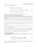
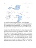
3. Numerical examples
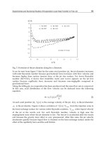
To verify the accuracy of the present method, unsteady heat conduction in a circular region
with radius a, as shown in Fig. 6, is treated with a boundary temperature given by
[1 cos( )]
H
TT t
. (92)
We assume an initial temperature T
0=0 C
, and R denotes the distance from the center of
the circular region. A two-dimensional state, in which there is no heat flow in the direction
perpendicular to the plane of the domain, is assumed. Figure 6 also shows the internal
points used for interpolation. A thermal diffusivity of
16 mm2/s and a radius of a=10
mm are assumed.
H
T
=10 C
in Eq. (92) and a frequency of /2
rad/s are also
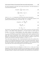
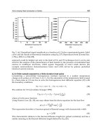
assumed. The BEM results at R
=0 and R=8 mm and the exact values are compared in Fig. 7.
The exact solution for the temperature distribution is given by (Carslaw, 1938)
22
(,) [1 cos
H
ber Rber a bei Rbei a
TRt T t
ber a bei a
Heat Conduction – Basic Research
342
Fig. 6. Circular region with temperature change at the boundary.
Fig. 7. Temperature history in circular region.
22
sin
ber Rbei a ber abei R
t
ber a bei a
3
2
2
0
'242
1
0
()
2
exp( ) ]
()( )
ss
s
s
ss
JR
t
a
Ja
(93)
where
ber(
) and bei(
) are Kelvin functions, and
s
( s=1, 2, ) are the roots of
0
()0Ja
.
Constant elements are used for boundary and time interpolation.
Meshless Heat Conduction Analysis by Triple-Reciprocity Boundary Element Method
343
Appendix A (3D)
The higher-order functions for 3D unsteady heat conduction are
*
2
,,,Tpqt
1/2
3/2
1
{(1.5,) [1exp()]}
2
aa a
r
3/2
1
(0.5, )
2
a
r
(A-1)
*
2
3/2 2
,,,
1
(1.5, )
2
Tpqt
r
a
nn
r
(A-2)
)]}exp(1[3
1
),5.1(3),5.2(3),2(6),5.1(3{
12
2/12/112/1
2/3
*
3
aa
a
aaaaaaa
r
T
)]}exp(1[2
1
),5.1(2),5.0({
4
2/1
2/3
aa
a
aa
r
(A-3)
.
n
r
a
a
a
n
T
)],5.1(
1
),5.0([
4
1
2/3
*
3
. (A-4)
where
(,)
is an incomplete gamma function of the first kind (Abramowitz, 1970) and
,/
ii
rrx
. Using Eqs. (44) and (A-3), the polyharmonic function with a surface
distribution is obtained as follows:
3/2
*3/23/2
32211212211
1/2
2( )
{2 (1.5,)2 (1.5,)2(3,)23, 6 (2,)6 (2,)
3
B
Akt
Tuuuuuuuuuu
r
1/2 1/2
2211
62.5,62.5,uuuu
22
21
11
22
uu
1/2 1/2
221121
61.5,61.5,6(2,)6(2,)uuuuuu
21 2 1
3 3 3exp( ) 3exp( )}uu u u
, (A-5)
where
2
1
()
4( )
rA
u
t
(A-6)
2
2
()
4( )
rA
u
t
. (A-7)
The time integral of Eq. (62) can be obtained as follows:
*
1
3/2
1
(,,,) (0.5, )
4
F
f
t
f
t
T
pq
td a
r
(A-8)
*
1
3/2 2
(,,,)
1
(1.5, )
2
F
f
t
f
t
Tpqt
r
da
nn
r
(A-9)
*
2
(,,,)
F
f
t
t
T
pq
td
3/2 1/2
12
[ (1.5, ) (0.5, ) ( 0.5, )]
8
ff f
f
f
r
aa a
a
a
Heat Conduction – Basic Research
344
3/2
1
[ (0.5, ) ( 0.5, )]
8
ff
f
r
aa
a
(A-10)
*
2
3/2
(,,,)
11
[ (1.5, ) (0.5, )]
8
F
f
t
ff
t
f
Tpqt
r
daa
nna
(A-11)
*
3
(,,,)
F
f
t
t
Tpqt d
3
3/2
1
[ 6 (1.5, ) (0.5, )
96
ff
f
r
aa
a
3/2
1
8(2, )
f
f
a
a
2
1
3(2.5, )
f
f
a
a
1/2
4
f
a
2
1
3(1.5, ) 3(0.5, )
ff
f
aa
a
3/2
4
6(1.5, )]
f
f
a
a
(A-12)
*
3
(,,,)
F
f
t
t
Tpqt
d
n
2
3/2
1
[6 (1.5, ) 3(0.5, )
96
ff
f
rr
aa
na
2
1
3(2.5, )
f
f
a
a
1/2
8
f
a
2
3
(1.5, ) 3 ( 0.5, )]
ff
f
aa
a
, (A-13)
where
2
4( )
f
F
f
r
a
tt
(A-14)
and
(,) is an incomplete gamma function of the second kind (Abramowitz, 1970). The time
integral of Eq. (A-5) can be obtained as follows:
*
3
(,,,)
F
f
t
B
t
T
pq
td
5
11
1/2
() 11
{2 (1.5, ) (0.5, )
5
48
ff
f
ArA
aa
a
r
1
5/2
1
41
(3, )
5
f
f
a
a
1
3/2
1
1
4(2, )
f
f
a
a
1
2
1
1
3(2.5, )
f
f
a
a
1/2
1
1
f
a
11
2
1
13
3 (1.5, ) ( 0.5, )
5
ff
f
aa
a
1
5/2
1
12 1
(2, )
5
f
f
a
a
3/2
1
2
f
a
1
3(2.5, )}
f
a
, (A-15)
where
2
1
()
4( )
f
F
f
rA
a
tt
. (A-16)
For the sake of conciseness, the terms involving
2
u in Eq. (A-5) are omitted. The derivative
of the polyharmonic function
*
(,,,)
f
TP
q
t
and the normal derivative with respect to
i
x
are
explicitly given by
*
1
35
22
exp( )
16 [ ( )]
ii
Tr r
a
xx
kt
(A-17)
Meshless Heat Conduction Analysis by Triple-Reciprocity Boundary Element Method
345
*
1
i
T
nx
35
22
1
2, ,exp()
16 [ ( )]
ijji
nurnr a
kt
(A-18)
*
2
3/2 2
13
,
2
2
ii
Tr
a
xx
r
(A-19)
*
2
i
T
nx
3/2 3
13 5
,2,,,
22
2
ii
jj
na arnr
r
(A-20)
*
3
3/2
1
11 3
,,
22
8
ii
T
r
aa
xux
(A-21)
2*
3
3
2
11 3
{ [ (0.5, ) (1.5, )] , , [ (0.5, ) (1.5, )]}
8
iijj
i
T
na arrna a
nx u u
r
(A-22)
*
3/2
3/2
3
11 1
1/2
2( ) 1
[ {2 (1.5, ) 2 3,
3
B
ii
dT
akt r
uu u
dx x r
r
11
6(2,)uu
1/2
11
62.5,uu
2
1
1
2
u
1/2
111
61.5,6(2,)uuu
11
33exp()}uu
1/2
11
1
2
{3 (1.5 , )
uu
r
1
6(2, )u
3/2
11
32.5,uu
1
3/2
11
31.5,uu
1
1
3u
1
11
3 exp( )}]uu
(A-23)
The time integrals of Eqs. (A-18), (A-20) and (A-22) can be obtained as follows:
*
1
F
f
t
t
i
T
d
nx
3
3
2
153
2, , , ,
22
2
ijj f i f
rnr a n a
kr
(A-24)
*
2
F
f
t
t
i
T
d
nx
3
2
113 11
(3,,) , ( ,,)[ ,]
222
8
iijj f iijj f
f
nrnr a nrnr a
a
kr
(A-25)
2*
21 1/2
3
3/2
21
(,,,)
311
3,6,3,16
222
192
311
,, 9 , 6 , 3 ,
222
F
f
t
if f f f f
f
t
i
ijj f f f f f
Tpqt
r
dnaaaaaa
nx
rrn a a a a a
(A-26)
*
3
F
f
t
B
t
i
T
d
x
4
1/2
211
{2 1.5, (0.5, )
32 5
3
ff
if
arr
aa
xk a
5/2
41
3,
5
f
f
a
a
3/2
1
42,
f
f
a
a
2
1
32.5,
f
f
a
a
1/2
1
f
a
Heat Conduction – Basic Research
346
2
13
31.5, 0.5,
5
ff
f
aa
a
5/2
12 1
2,
5
f
f
a
a
2/3
2
f
a
3(2.5,)}
f
a
(A-27)
Appendix B (1D)
The functions for 1D unsteady heat conduction are
*
2
,,,Tpqt
12
12
(,0.5) exp( )
2
r
aa a
(B-1)
*
2
1/2
,,,
1
(0.5, )
2
Tpqt
r
a
nn
(B-2)
3
*11/23/23/2
3
12
, , , {( 1.5) (0.5, ) exp( ) 2 exp( )}
12
r
T
pq
taaaaaaaa
(B-3)
*
2
3
11
12
,,,
[(1 ) (0.5, ) (1.5, )]
4
Tpqt
rr
aaaa
nn
, (B-4)
where
(,)
is an incomplete gamma function of the first kind (Abramowitz, 1970). The time
integral of Eqs. (49) and (B-1)-(B-4) can be obtained as follows:
1
12 0.5
1exp( )
(,,,) [(0.5, ) ]
2
F
f
t
f
f
t
f
a
r
Tpqt d a
a
(B-5)
*
1
(,,,)
F
f
t
t
Tpqt
d
n
12
1
(0.5, )
2
f
r
a
n
(B-6)
*
2
(,,,)
F
f
t
t
Tpqt d
12 32
3
12 2
()
122
(0.5, ) (0.5, ) exp( )
33
8
ff
ff f
f
f
aa
r
aa a
a
a
(B-7)
*
2
(,,,)
F
f
t
t
Tpqt
d
n
2
12 12
11
{ (0.5, ) 2[ (0.5, ) exp( )]}
8
ff f
f
f
rr
aa a
na
a
(B-8)
5
*
3
12
2
1/2 3/2 5/2 5/2
34
( , , , ) {15( ) (0.5, ) 12 (0.5, )
2880
294 48
12 (0.5, ) 6( )exp( ) }
F
f
t
ff
t
f
f
ff
f
fff
r
Tpqt d a a
a
a
aa
aaa a
(B-9)
*
4
3
12 2 12 32
exp( ) 2exp( )
(,,,)
11 1
{( ) (0.5, ) (0.5, ) }
3
2
16 3 3
F
f
t
ff
ff
t
f
f
ff
aa
Tpqt
rr
daa
nna
a
aa
, (B-10)
Meshless Heat Conduction Analysis by Triple-Reciprocity Boundary Element Method
347
where
2
4( )
f
F
f
r
a
tt
. (B-11)
Appendix C (Linear time interpolation)
The time integrals of Eq. (62) using linear time interpolation in the two-dimensional case can
be obtained as follows:
1
22
1
*
1 11 1
1
exp( ) exp( )
1
() ( ) ()()
44 4
f
f
t
ff
fFfff
t
ff
aa
rr
tTd tt Ea Ea
aa
(C-1)
1
22
1
*
11 1 1 1 1
1
exp( ) exp( )
1
() ( ) ()()
44 4
f
f
t
ff
fFfff
t
ff
aa
rr
tTd tt Ea Ea
aa
(C-2)
1
*
1
()
f
f
t
f
t
T
td
n
1111
2
11 1
()exp()exp() ()()
24
Ff f f f f
r
t t a a Ea Ea
n
R
(C-3)
1
*
1
1
()
f
f
t
f
t
T
td
n
11 111
2
11 1
()exp()exp() ()()
24
Ff f f f f
r
tt a a Ea Ea
n
R
(C-4)
1
*
2
()(,,,)
f
f
t
f
t
tTpqtd
2
1
1
()ln() 1exp( )
16( ) ( )
256
ff f
Ff f
f
Ea a C a
r
ttEa
a
2
1
1
2
1exp( ) 2()2ln( )2 1exp( )
()
fff ff
f
f
f
aEa aC aa
r
Ea
a
a
2
111 1 1 1
11
2
1
1
1exp( ) 2( )2ln( )2 1exp( )
()
fff ff
f
f
f
aEa aC aa
r
Ea
a
a
(C-5)
1
*
12
()(,,,)
f
f
t
f
t
tTpqtd
2
1
11
()ln() 1exp( )
16( ) ( )
256
ff f
Ff f
f
Ea a C a
r
tt Ea
a
2
1
1
2
1exp( ) 2()2ln( )2 1exp( )
()
fff ff
f
f
f
aEa aC aa
r
Ea
a
a
Heat Conduction – Basic Research
348
2
111 1 1 1
11
2
1
1
1exp( ) 2( )2ln( )2 1exp( )
()
fff ff
f
f
f
aEa aC aa
r
Ea
a
a
(C-6)
1
*
1
2
11 1
1
1exp( ) 1exp( )
() ()() ()()
8
f
f
t
ff
fffff
t
ff
aa
Trr
t d t t Ea tt Ea
nn a a
2
1
2
11 11 1
2
2
2
2
2( )
{1 exp( ) exp( ) exp( )}
2( )
{1 exp( ) exp( ) exp( )}
f
ff ff f
f
ff ff f
tt
aa aa a
r
tt
aa aa a
r
(C-7)
1
4
*
311
1
()(,,,) {36( ) 4()4ln()4exp()1
9216
f
f
t
fFfffff
t
f
r
tTpqtd ttEa Ea aC a
a
1
2
2()2ln()2 3exp( )35
ff ff
f
Ea a C a a
a
()
11 11 1 1
1
1
() 4()4ln 41exp
fff f
f
Ea Ea a C a
a
1
2
1
2()2ln()2 3exp( )35
ff ff
f
Ea a C a a
a
2
1
11
1exp( )
()
f
f
f
a
r
Ea
a
11 1 1 1
2
1
18 ( ) 18ln( ) 18 1 exp( )
ff f f
f
Ea a C a a
a
2
11 1 1 1 1
3
1
12 ( ) 12ln( ) 12 16 16exp( ) 28 11
ff fff
f
Ea a C a a a
a
1
9exp( )
()
f
f
f
a
Ea
a
1
2
18 ( ) 18ln( ) 18 9 exp( ) 27
ff ff
f
Ea a C a a
a
1
3
12 ( ) 12ln( ) 12 16 16exp( )
}
ff f
f
Ea a C a
a
(C-8)
Meshless Heat Conduction Analysis by Triple-Reciprocity Boundary Element Method
349
1
*
3
()
f
f
t
f
t
T
td
n
5
111 1
11
22
1
1
exp( ) ( ) ln( )
() 6
1536
fff
f
f
f
aEa aC
rr
Ea
na
a
111
23
11
1exp( ) 1exp( )
4
fff
ff
aaa
aa
11 1 1
11
2
11
24 ( ) ( ) ln( ) 1 exp( )
()2
Ff f f f
f
ff
tt Ea a C a
Ea
aa
r
11
2
1
1exp( )
ff
f
aa
a
1
1
2
exp( ) ( ) ln( )
() 6
fff
f
f
f
aEa aC
Ea
a
a
23
1exp( ) 1exp( )
4
fff
ff
aaa
aa
1
1
2 2
24( ) ( )ln( ) 1exp( ) 1exp( )
()2
Ff f f f f f
f
ff
f
tt Ea a C a a a
Ea
aa
ra
. (C-9)
4. References
Abramowitz, M. and Stegun, A. Eds., (1970), Handbook of Mathematical Functions, pp. 255-263,
Dover, New York.
Brebbia, C. A., Tells, J. C. F. and Wrobel, L. C., (1984), Boundary Element Techniques-Theory
and Applications in Engineering, pp. 47-107, Springer-Verlag, Berlin.
Carslaw, H. S. and Jaeger, J. C., (1938), Some Problems in the Mathematical Theory of the
Conduction of Heat, Phil. Mag., Vol. 26, pp. 473-495.
Dyn, N., (1987), Interpolation of Scattered Data by Radial Functions, in Topics in Multivariate
Approximation, Eds. C. K. Chui, L. L. Schumaker and F. I. Utreras, pp. 47-61,
Academic Press, London.
Micchelli, C. A., (1986), Interpolation of Scattered Data, Constructive Approximation, Vol. 2, pp.
12-22.
Nowak, A. J., (1989), The Multiple Reciprocity Method of Solving Transient Heat
Conduction Problems, Advances in Boundary Elements, Vol. 2, pp. 81-93, Eds. C. A.
Brebbia and J. J. Connors, Computational Mechanics Publication, Southampton,
Springer-Verlag, Berlin.
Nowak, A. J. and Neves, A. C., (1994), The Multiple Reciprocity Boundary Element Method,
Computational Mechanics Publication, Southampton, Boston.
Ochiai, Y. and Sekiya, T., (1995a), Steady Thermal Stress Analysis by Improved Multiple-
Reciprocity Boundary Element Method, Journal of Thermal Stresses, Vol. 18, No. 6,
pp. 603-620.
Ochiai, Y., (1995b), Axisymmetric Heat Conduction Analysis by Improved Multiple-
Reciprocity Boundary Element Method, Heat Transfer-Japanese Research, Vol. 23, No.
6, pp. 498-512.
Ochiai, Y. and Sekiya, T., (1995c), Generation of Free-Form Surface in CAD for Dies,
Advances in Engineering Software, Vol. 22, pp. 113-118.
Heat Conduction – Basic Research
350
Ochiai, Y., (1996a), Generation Method of Distributed Data for FEM Analysis, JSME
International Journal, Vol. 39, No. 1, pp. 93-98.
Ochiai, Y. and Sekiya, T., (1996b), Steady Heat Conduction Analysis by Improved Multiple-
Reciprocity Boundary Element Method, Engineering Analysis with Boundary
Elements, Vol. 18, pp. 111-117.
Ochiai, Y. and Kobayashi, T., (1999), Initial Stress Formulation for Elastoplastic Analysis by
Improved Multiple-Reciprocity Boundary Element Method, Engineering Analysis
with Boundary Elements, Vol. 23, pp. 167-173.
Ochiai, Y. and Yasutomi, Z., (2000), Improved Method Generating a Free-Form Surface Using
Integral Equations, Computer Aided Geometric Design, Vol. 17, No. 3, pp. 233-245.
Ochiai, Y., (2001), Two-Dimensional Unsteady Heat Conduction Analysis with Heat
Generation by Triple-Reciprocity BEM, International Journal of Numerical Methods in
Engineering, Vol. 51, No. 2, pp. 143-157.
Ochiai, Y., (2003a), Multidimensional Numerical Integration for Meshless BEM, Engineering
Analysis with Boundary Elements, Vol. 27, No. 3, pp. 241-249.
Ochiai, Y., (2003b), The Multiple-Reciprocity Method for Elastic Problems with Arbitrary
Body Force, Transformation of Domain Effects to the Boundary, Y. F. Rashed Ed.,
Chapter 5, ISBN 1-85312-896-1, WIT Press.
Ochiai, Y. and Sladek, V., (2005), Numerical Treatment of Domain Integrals without Internal
Cells in Three-Dimensional BIEM Formulations, CMES(Computer Modeling in
Engineering & Sciences) Vol. 6, No. 6, pp. 525-536.
Ochiai, Y., Sladek, V. and Sladek, S., (2006), Transient Heat Conduction Analysis by Triple-
Reciprocity Boundary Element Method, Engineering Analysis with Boundary
Elements, Vol. 30, No. 3, pp. 194-204.
Ochiai, Y and Takeda, S., (2009a), Meshless Convection-Diffusion Analysis by Triple-
Reciprocity Boundary Element Method, Engineering Analysis with Boundary
Elements, Vol.33, No.2, pp.168-175.
Ochiai, Y and Kitayama, Y., (2009b),Three-dimensional Unsteady Heat Conduction Analysis
by Triple-Reciprocity Boundary Element Method, Engineering Analysis with
Boundary Elements, Vol. 33, No. 6, pp. 789-795.
Partridge, P. W., Brebbia, C. A. and Wrobel, L. C., (1992), The Dual Reciprocity Boundary
Element Method, Computational Mechanics Publications, pp. 223-253.
Sladek, J. and Sladek, V., (2003), Local Boundary Integral Equation Method for Heat
Conduction Problem in an Anisotropic Medium, Proceedings of ICCES2003, Chap. 5.
Tanaka, M., Matsumoto, T. and Takakuwa, S., (2003), Dual Reciprocity BEM Based on Time-
Stepping Scheme for the Solution of Transient Heat Conduction Problems,
Boundary Elements XXV, WIT Press, pp. 299-308.
Wrobel, L. C., (2002), The Boundary Element Method, Vol. 1, John Wiley & Sons, West Sussex, pp.
97-117.