Environmental Monitoring Part 15 pptx

Environmental Monitoring WSN

481
of power, taken from the battery power available. Introducing several intelligent features to
each sensor is also limited due to the power constraint.
Each source can transmit the data directly to the base station if the sources are located
within the base station’s communication range. Some examples of existing applications
deploying single-hop communication (Mainwaring et al., 2002; Martinez et al., 2005;
Jovanov et al., 2003; Otto et al., 2006). For single-hop, the sources are located within the base
station’s range. Direct communication is therefore feasible and several benefits are realised.
One of the advantages is the ability to introduce a variety of intelligent features to the base
station as it is assumed to have more power and computational capabilities compared to an
ordinary sensor. Each source does not require the power necessary for routing. Idle listening
can be minimised as the sources can be switched to sleep mode if they do not transmit data
or receive the control packet. The base station controls the communication schedule of its
sources to avoid data collisions. Power for carrier sensing is not desired. In multi-hop, each
source is responsible for sensing, data reporting and routing. The number of transmissions
and receptions increases with the number of intermediary nodes required for data
forwarding.
This work looks at protocol development for single-hop. A scenario where the single-hop is
viable is Environmental Monitoring (EM). Sources and base stations are distributed and
several clusters or patches are formed. A power-aware, single-hop protocol can thus be used
in each of the clusters (Mainwaring et al., 2002). A low duty cycle is the norm in EM so the
communication cycle of each source can be scheduled by the base station. A time slot is
allocated to each source to perform data transmissions. Carrier sensing is thus not required
in this scheme. The sources synchronise to the base station by checking the information
included in the control packet.
2.4 Reliability
Wireless sensor network (WSN) has been currently deployed in several civil applications.
The physical data is collected and transmitted for further analysis. The issue of reliability in

data delivery is important for providing complete reliability consumes a significant
proportion of power. Applying the Transmission Control Protocol (TCP) protocol to WSN is
expensive because of its three-way handshake mechanism and packet header size. The User
Datagram Protocol (UDP) is considered to be more suitable for sensors although it was
designed to provide unreliable data transport. In some applications, data loss may be not a
serious problem because of the large amount of deployed sensors. Reliable data transport is
important for some types of data such as control messages delivered by the base station
(Wan et al., 2002). The following paragraphs provide some details of reliable transport
protocol for WSN researches including PSFQ (Pump Slowly, Fetch Quickly) (Wan et al.,
2002), ESRT (Event-to-Sink Reliable Transport) (Sankarasubramaniam et al., 2003), and
RMST (Reliable Multi-Segment Transport) (Stann & Heidemann, 2003).
One of the main goals to achieve reliable data transport is to orchestrate data receiving and
forwarding processes to lessen the packet loss due to buffer overflow. PSFQ proposes three
different operations including pump, fetch and report. Data generated from a source node is
injected slowly into the network in order to allow such nodes experiencing data loss to fetch
the missing packets very aggressively. Timing is a core process in order to avoid operational
synchronisation. A hop-by-hop recovery is applied to avoid exponential error accumulation
as occurs in the end-to-end scheme. Data delivery status information can be sent back to
users or applications in a piggyback fashion.

Environmental Monitoring

482
Focusing only on the forward or sensor-to-sink direction, ESRT was designed to provide a
reliable data transport by inspecting current network state in terms of reliability and
congestion. The state result is categorised and the reporting frequency is then repetitively
adjusted to reach an optimal point. ESRT provides both reliable data transport and
congestion control. Local buffer level monitoring is used to detect congestion.
Directed Diffusion (Intanagonwiwat et al., 2003) is a routing protocol which provides a
multipoint-to-multipoint communication. A sink firstly indicates an interest and propagates

it to the nodes. Interest and node information is kept as gradients. The optimised reinforced
path is then established to send the attribute-value pairs data. RMST is implemented as a
filter to provide some information about the data fragment such as ID and total number of
fragments to detect loss. A NACK (Negative ACKnowledgement) is sent via a back-channel
to upstream neighbouring nodes in case of data loss.
According to the above fundamental protocol descriptions, several conclusions can be made.
In a densely deployed environment, data loss may be accepted. However, this condition
may apply only in the case of sensor-to-sink traffic. The sink or base station plays a major
role in the network by broadcasting several control packets to the sensors. Such packets
should not be lost. Moreover, there are various types of sensing data, such as structural
displacement due to wind or earthquake (Xu et al., 2004), which need some combination
from different nodes to create usable data before forwarding that data to the sink. PSFQ
designing concepts are more complicated but can be applied to a broader area of
application. The data retransmission mechanisms are not mentioned in ESRT as it focuses on
statistical reliability. However, PSFQ does not provide congestion control schemes as ESRT
does. RMST is designed to run over the Directed Diffusion routing protocol. Although it
may take the least effort compared to the other two, it is not generic enough.
3. Resource constraint issues
This section introduces several issues of resource constraint in WSN. A sensor can be
considered as a small computing device which is capable of sensing, data processing,
storage and communication. Sensors are deployed in an area of interest and they may have
to operate without maintenance throughout their lifetimes. Power is thus one of the limited
resources. Unless an external source of energy is provided, power for all operations comes
from batteries. Two AA batteries are required in the widely used platforms such as Tmote,
Telos and Mica. The capacity of the AA battery is approximately 2,000 to 3,000 milli-ampere-
hour (mAh). In order to calculate the battery life, the capacity is divided by the actual load
current and the obtained lifetime is in hours. An equation for calculating sensor’s lifetime is
given in (Polastre et al., 2004) where the lifetime is equal to the product between capacity
(mAh) and voltage (3V) divided by total energy consumption in micro-joules. The default
capacity defined in (Polastre et al., 2004) is set at 2,500mAh.

Communication accounts for a significant proportion of energy consumption. There are four
main modes of communication including sending, receiving, sleeping and listening. The
transceiver is one of the major sensor components and it makes them capable of
communicating with other nodes. Recent transceivers or radio chips such as CC1000 and
CC2420 provide programmable transmission power. Sensors consume less power when
they send at a lower power level. Hence, transmission power control is one of power-aware
schemes in WSN. The sensors do not always send at the maximum power. Tmote platform
is chosen in this study and it employs CC2420 transceiver. For the CC2420 mote the

Environmental Monitoring WSN

483
minimum and maximum transmission power is 8.5 and 17.4 milli-amperes (mA). Over 50%
of the power can be saved if the minimum power is always used.
Sensors equipped with CC2420 radio chips consume a greater amount of power when they
receive data. According to the data sheet, 19.7mA is required for reception. Listening and
sleeping consume 365 and 20 micro-amperes (µA), respectively. Hence, in the case of the
CC2420 mote, data reception consumes more energy than transmission. The base station is
the destination and it may be connected to a desktop or laptop computer. In such cases, the
base station has extra power from the connected machine. However, the sensors which act
as intermediary nodes between source and destination have to receive and forward packets
resulting in sensor’s lifetimes being decreased. The listening power is approximately 17
times greater than sleeping. In some applications such as environmental monitoring, the
data sampling interval may be in minutes or hours. The transceivers should be switched to
sleep mode instead of listening. Scheduling issues occur when two nodes communicate with
each other. The data is not received if the receiver is in sleep mode. The nodes have to agree
upon the same scheduling. Another scheme based upon contention-based can be used; the
receiver can periodically listen to the signal propagated over the medium to inspect whether
the incoming message is destined for it.
WSN is also a shared medium system. Each of the sources and base station has to engage the

medium to perform data communication. Data collisions occur if the sources transmit at the
same time and energy will be wasted by unsuccessful data delivery. A Medium Access
Control (MAC) protocol is required to resolve the contention. The features of the MAC
protocol together with the application behaviour determine when a node is idle, when it is
listening and when it is sending. As each of these states have different power requirements
the MAC protocol impacts upon the efficiency of operation and the power consumption.
There are two main MAC schemes; the contention and the schedule based. The medium is
sensed prior to transmission and the sensors have to backoff if the medium is declared busy.
This work focuses on the single-hop where the sources send data directly to the base station.
Another scheme, schedule based, is adopted. A data slot is allocated to each node. No
carrier sensing and corresponding energy is required. The main issue is that the slot must be
long enough for completing data delivery, otherwise, data collisions are likely.
Experimentations required to determine the duration required for both sending and
receiving together with the effective factors such as data payload size. Each node is switched
to sleep mode to spend the least amount of power when its slot does not arrive.
The buffering capacity of CC2420 is limited to 128 bytes. Taking the header’s and footer’s
sizes into account, the allowable data payload size is thus less than 128 bytes. Apart from
sensed data, some control information is required in the packet such as identification and
timestamp. Additional packet structures may be required if all the information cannot be
stored in one packet. Control overhead is considered as one of the costs and should be
minimised in order to decrease transmission and reception energy.
Wireless sensor network (WSN) has been currently deployed in several surveillance and
civil applications. Sensors may be scattered over an area of interest which can be very large.
The communication range is thus important and depends upon the selected transceiver. For
example, the CC2420 mote has 50m and 125m indoor and outdoor ranges. Under some
circumstances, the maximum transmission power may not produce the maximum ranges.
Furthermore, sending data to the node located at farther distances requires higher
transmission power. Multi-hop is therefore usually used in WSN. Several intermediary
sensors are required for data forwarding from the source to destination. Single-hop

Environmental Monitoring

484
communication is feasible if the destination is located within the source’s range. Multiple
transmissions and receptions are not required if direct communication applies. However,
the same transmission power cannot always be used as the link quality changes over time.
The next section describes several sources of variability in radio frequency
4. Motivation of PoRAP development
This work aims at building a communication protocol for WSN. The targeted scenario is the
periodic-based where a low duty cycle is required. The network consists of a fixed set of
sources and a base station. Furthermore, direct data communications between the base
station and its sources are feasible. The communication protocol to be developed will
effectively support the single-hop WSN. Such a structure forms a network cluster which can
be used in some environmental or habitat monitoring system such as (Mainwaring et al.,
2002) and (Tolle et al., 2005). As the number of sources is fixed throughout the
communications, the data reporting rate is fairly constant. The communication of the
sources can be therefore scheduled and controlled by the base station. A time slot is
allocated to each source and will be used for data communication. Only one source can use
the shared medium whilst the others switch to sleep mode by turning their radios off and
consuming the least amount of energy. Data collision can be avoided and idle listening can
be minimised.
4.1 Sensor node power consumption
This section establishes the significance of network communication as a consumer of energy
within a wireless sensor network. In doing so a careful reading of sensor data sheets is used
to inform calculations based upon the sensor’s parameters and simulations. What
proportion of the power is used for communication is investigated and how power may be
conserved is identified.
In order to investigate how power is consumed by a sensor, a simulation study has been
established. The results are validated by the CC1000 transceiver data sheet. As the sensor
operating system used in this work is TinyOS, the selected simulator is TOSSIM which is a

TinyOS library. TinyOS is an operating system specifically designed for embedded devices
such as sensors. It has been widely used in both research and commercial communities. The
selected release of the simulator is TOSSIM 1 and it does not provide power usage
measurement capability. PowerTOSSIM, an extension module developed for analysing
power consumption of hardware components (Shnayder et al., 2004) is used to address the
investigation on power consumption and it is included in Tiny 1.1.11. The only sensor
platform supported in PowerTOSSIM is Mica2 which employed the CC1000 radio chip. The
PowerTOSSIM supports an operating frequency of 400 Megahertz (MHz) and a voltage of 3
Volt. The energy model file of PowerTOSSIM adopts the required transmission current for
each power level. According to the CC1000 datasheet, 31 output power levels ranging from -
20 to +10dBm can be programmed. The dBm is the measurement of power loss in decibels
(dB) using 1 milli-watt (mW) as a reference value.
4.1.1 Simulation parameters
A sensor node was created in the simulation and performs as a transmitting node. An
experiment was conducted to obtain the current consumption required by each transmission
power level. In total five transmission powers including -20, -10, 0, +6 and +10dBm were

Environmental Monitoring WSN

485
used. The corresponding current consumption was measured by (Shnayder et al., 2004) and
their results are shown in Table 1. A simulation duration of 60 seconds and a total of 30 runs
were conducted at each power level. A higher current will be consumed if the sensor
transmits at a higher power.

Transmission Power (dBm) Required Current (mA)
-20 5.21
-10 6.10
0 8.47
+6 13.77

+10 21.48
Table 1. Current consumption measured by Shnayder et al., 2004
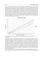
The results shown in Table 1 were used to compute the energy consumption required by
each transmission power level. Fig. 1 shows error-bar plots of radio and total energy
consumption at -20, -10, 0, +6 and +10 dBm. An analysis of power usage and conservation
with respect to the maximum power level is described in Table 2.
According to Fig. 1, several observations can be made. Firstly, an increase in transmission
power results in a higher energy consumption. Transmitting data at lower power uses less
energy. For example, over 75% of energy can be conserved if the minimum power is used
for transmission instead of the maximum. Secondly, the radio unit consumes a significant
amount of energy. Up to 56% and 84% of energy are used by the radio if the sensor
transmits at minimum and maximum power levels, respectively. The results are validated
by the CC1000 data sheet which is the employed radio in Mica2. According to the CC1000
datasheet, the required current consumption for -20 and +10 dBm are 6.9 and 26.7 milli-amp
(mA), respectively. Therefore, over 74% can be conserved and this is close to the 75% which
is obtained from PowerTOSSIM.


Fig. 1. Radio and total energy consumption at various transmission power levels

Environmental Monitoring

486

Transmission Power
(dBm)
Average of Radio
Power Consumption
(mJ)
Percentage of Used

Power
Percentage of Saved
Power
-20 861.52 24.67 75.33
-10 1000.33 28.64 71.36
0 1396.44 39.98 60.02
+6 2236.90 64.05 35.95
+10 3492.48 100 0
Table 2. Average radio power consumption (mJ) and percentages of used and saved power
Two key motivations are established with respect to the simulation results. Firstly,
transmission power considerably affects radio power consumption. The power-aware
approach based upon power adaptation is Transmission Power Control (TPC). PoRAP
adopts the TPC concepts in order to achieve the power conservation goal. The selected
sensor platform in this work is Tmote and it employs the CC2420 radio instead of the
CC1000. Like the CC1000, the CC2420 also supports transmission power adaptation but it
provides a different range of power levels. Table 3 shows some of the possible power levels
and the corresponding current consumption. An analysis of power conservation with
respect to the maximum level is also shown.

Transmission Power
(dBm)
Current Consumption
(mA)
Percentage of Used
Current
Percentage of Saved
Current
-25 8.5 48.85 51.15
-15 9.9 56.90 43.10
-10 11.2 64.37 35.63

-7 12.5 71.84 28.16
-5 13.9 79.89 20.11
-3 15.2 87.36 12.64
-1 16.5 94.83 5.17
0 17.4 100 0
Table 3. Transmission power levels provided by CC2420 and analysis of power conservation
According to Table 3, over 50% of power can be saved if the minimum power is used for
data transmission. The transmission power is one of the main factors which produces
different reception strengths. The power adaptation is based upon the current link quality in
order to maintain a good link. However, power adaptation is based upon several factors
affecting link quality such as distance and time-of-day.
Secondly, according to Fig. 1, the radio unit accounts for a significant amount of power
compared to the total consumed by all hardware components. Keeping the radio in sleep
mode after the sensor has transmitted the data may establish an enhancement in power
conservation. This is feasible if the single-hop network sensors do not listen to transmissions
from other nodes in order to discover optimal data paths. The schedule-based MAC
(Medium Access Control) approach suits the direct communication scenario as each of the
sources wake up for control reception and data transmission. Otherwise, they are in sleep
mode and consume the least amount of communication energy.

Environmental Monitoring WSN

487
4.2 Environmental investigation of transmission power and reliability
This section provides details of experimental studies aimed at establishing effects of
transmission power, distances and time-of-day on link quality metrics. In total three metrics
including RSSI (Received Signal Strength Indicator), LQI (Link Quality Indication) and PRR
(Packet Reception Rate) are used to describe the effects. The relationships between the
metrics are also investigated and will be used for establishing power adaptation policies.
4.2.1 Link quality metrics

There is a variety of sources which cause variability in link quality in wireless communication.
Unlike wired communication, environmental factors such as climatic conditions and time-of-
day also affect the degree of signal attenuation. A significant degree of signal attenuation or
interference may lead to unsuccessful data transmission. Link quality measurement is
therefore one of the major issues in wireless network communication.
A transmitter sends data packets at a specific transmission power wirelessly over a medium
to a receiver. The transmission power level is programmable and this capability is provided
by a transceiver or radio unit which is a component responsible for data transmission and
reception. A sensor communicates with the other node by sending and receiving messages
via wireless channel which is normally air. Several signals are generated from various
sources such as electronic appliances and they are dissipated to the air. A wireless channel
may then have background noise which is capable of interfering with data delivery between
a pair of nodes. Moreover, time-of-day and climatic conditions such as fog and rain affects
the wireless link quality. In order to determine link quality characteristics, all causes of
signal strength reduction are considered as sources of signal attenuation. The reduced
magnitude in signal strength is therefore defined as signal attenuation. If the transmission
power is less than signal attenuation, the message cannot be successfully received. When the
receiver is not able to receive the sent packet and the number of received packets is not
increased, the reliability requirement defined by an application may not be met.
Transmission power should be adjusted in response to the changing link quality.
A radio unit provides several mechanisms to measure received signal power. The measured
values are categorised as received signal strength (RSS). In total two attributes including
RSSI (Received Signal Strength Indicator) and LQI (Link Quality Indication) are in the RSS
category. The RSS can be used to indicate link quality. The reliability requirement specified
by an application indicates a required number of packets received at the base station. The
percentage of data receptions can be used to describe the link quality. The packet reception
rate (PRR) is therefore introduced. Relationships amongst transmission power (TX),
received signal strength (RSS) based attributes and PRR is useful for mapping application
requirements to link quality measurements. Thus, the transmission power is adapted in
order to provide reliability of packet reception.

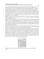
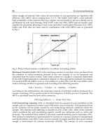
Received Signal Strength Indicator (RSSI) is defined as a measurement of the signal strength
of an incoming message. The transmitted signal strength or transmission power reduces as
the signal propagates through the medium. The RSSI is measured at the receiver and it
demonstrates the received signal strength. Therefore, signal attenuation is approximately
the difference between the transmission power and the RSSI. Link Quality Indication (LQI)
is another metric in the RSS-based category. According to the definition outlined in IEEE
802.15.4 Standard for Local and Metropolitan Area Networks, the LQI measurement is a
characterisation of the strength and/or quality of received packet. Each received packet has
its own LQI measurement and the integer value ranges from 0 to 255. Therefore, the

Environmental Monitoring

488
minimum and maximum values of LQI for each packet are 0 and 255, respectively. The IEEE
standard recommends at least eight unique values of LQI should be used in order to yield a
uniform distribution between the two limits. The following details of LQI are based upon
the CC2420 radio unit as it is used in both Tmote Sky and Tmote Invent which are the
chosen platforms in this research. Apart from RSSI and LQI, PoRAP determines an
additional link quality index. The main reason is that both RSSI and LQI are not transparent
to the user or application. Mapping mechanisms are required in order to convert an
application requirement to the ranges of RSSI and LQI values the base station should have.
This subsection aims to describe the Packet Reception Rate (PRR) which is more closely
related to the application requirement. In this research, the PRR is defined as a percentage of
the number of correctly received to that of transmitted packets. The PRR value is in the
range of 0% to 100%. The 100% PRR indicates complete reliability. Each received packet has
its own measured RSSI and LQI which can be used to predict the PRR. Models representing
relationships amongst metrics are therefore required and demonstrated later in this chapter.
4.2.2 Experimental setup
In our implementation-based experiments, Tmote Invent and Tmote Sky are used as the
sensor and base station, respectively. Both of them employ the CC2420 radio which has

working frequency band from 2,400 to 2,483 Megahertz (MHz). The radio transmission data
rate is 250 kilobits per second (kbps). The random access memory (RAM) and program flash
sizes are 10 and 48 kilobytes (Kbytes). The main difference between both platforms is that
the Tmote Invent provides built-in sensor and battery boards. The minimum and maximum
transmission power levels are -25 and 0dBm, respectively. Tmote sensors consume 8.5 and
17.4 milli-amps (mA) for transmitting a data packet at minimum and maximum power
levels, respectively. A current of 19.7mA is required for radio receiving. This indicates that
receiving accounts for a large radio power usage. Listening removal in PoRAP may enhance
power conservation in WSN. Each Tmote sensor includes an internal Inverted-F antenna
which is a wire monopole. The top section of the antenna is folded down to be parallel with
the ground plane. The communication ranges for indoor and outdoor are 50m and 125m,
respectively.
The experiments were conducted in the 16m x 20m indoor environment. The base station
was plugged into a desktop computer and received data from sensors. Three sensors were
used and they were placed at the same locations. In total 10 locations including 1, 2, 3, 4, 5, 7,
10, 13, 16 and 20m were used. The sensors and base station had the same antenna
orientation and height above floor level. The payload size was 12 bytes. In total 8
transmission power levels including 3, 7, 11, 15, 19, 23, 27 and 31 associated to -25, -15, -10, -
7, -5, -3, -1 and 0 dBm were used. The sensors transmitted one packet every second. At each
power, the sensors transmitted 50 packets for statistical analysis. Upon data reception, the
base station measured RSSI and LQI. The number of received packets was counted in order
to compute PRR.
4.2.3 Experiments on location as a determination of necessary transmission power
The significance of the locations of the sending and receiving motes to determine the
relationship between transmission power (TX) and reception quality is established. In this
experiment, the base station location was the same whilst three sensors were placed at 10
different locations in the same direction with clear line-of-sight (LOS) including 1, 2, 3, 4, 5,
7, 10, 13, 16 and 20m. Each power adaptation cycle was ended after the maximum power

Environmental Monitoring WSN

489
had been reached. The other experimental parameters such as power levels, data sending
rate and number of runs are stated in Section 4.2.2.
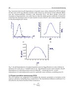
Fig. 2 shows the average RSSI readings of the three sensors at various locations and
transmission power levels. The missing data indicate that the power provides RSSI reading
less than -95dBm which is the minimum value reported by TinyOS. Fig. 3 shows average
LQI readings of a sensor at various locations and transmission power levels. The missing
data indicate unsuccessful data delivery.


Fig. 2. Effects of sensor locations on RSSI


Fig. 3. Effects of sensor locations on LQI

Environmental Monitoring

490
According to Fig. 2 and Fig. 3, most of the RSSI measurements proportionally increased with
the transmission power levels. Unlike the RSSI, the LQI measurements were stable at closer
locations especially when higher power was used for transmission. Most of the LQI values
decreased at greater distances. The minimum power level of -25dBm could be used to
successfully deliver data to the base station only when the locations were within 7m. The
decrease in received signal strength with increasing distances assumed in the prediction
models do not apply in the results. For example, in the case of 2m, the sensor provides a
weaker strength compared to a distance of 3m. The experimental results given in (Lin et al.,
2006) and (Stoyanova et al., 2007) demonstrate similar observations on location effects. The
RSSI and LQI are measured only when the base station receives data. The observed
minimum RSSI values higher than -95 dBm indicate data reception.

4.2.4 Fluctuation in link quality metrics over time of day
This section investigates on how RSSI, LQI and PRR fluctuate over the time of day. The
same base station and Sensor 1 were used. The sensor was located at 20m in the same
environment. It transmitted one packet every second at 0 dBm for 1,440 minutes or 24 hours.
The experiment was started in the morning before the office hour.
Fig. 4 demonstrates fluctuation of the RSSI, LQI and PRR over time of day. The RSSI
fluctuated during the first half of the experiment. It was stable during the night time and the
fluctuation was back later in the experiment. Unlike the RSSI, the LQI fluctuated throughout
the experiment. At the beginning the PRR siginificantly decreased. This observation was
resulted from the presence of people around the lab. The PRR increased during the night
time as there were no staff and student in the lab.
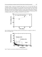
In summary, apart from transmission power, location and heterogeneity in the manufacture,
the link quality metrics are affected by the time-of-day. The presence of people around the
lab is the main factor in this experiment and is considered as temporary physical barrier.
Radio communication in WSN requires a line-of-sight. Some packets may be lost if there are
some people in the sending path.
4.2.5 Relationship between metrics
This section aims to describe the relationships between RSSI, LQI and PRR. During packet
reception, the base station measures RSSI and LQI. Apart from RSSI and LQI, the standard
message type of TinyOS includes the CRC field which is a Boolean data type. The base
station also looks at the CRC field to see if the data packet is received correctly. The
numbers of data transmissions and receptions are counted to compute the PRR. This scheme
can be used in a long-term operation.
However, the PRR may be estimated from the RSSI or LQI measurements. This concept suits
a short term operation. The base station does not count the numbers of sent and received
packets. Hence, the relationship between metrics needs to be established. Fig. 5 shows
relationships between the link quality metrics at 5m, 12m and 19m. The average RSSI and
LQI are computed at each transmission power level. The number of received packets is
counted in order to calculate the PRR.
According to Fig. 5, several observations can be made as follows:

1. The PRR steeply increases with RSSI up to a certain point followed by more stable
reliability measurements. Significant variations in reception rates are found when the RSSI
readings are between -95 and -90 dBm. At least 95% PRR may be achieved at all distances
if the sensor transmits data at the power producing RSSI greater than -90 dBm.

Environmental Monitoring WSN

491
2. The higher LQI results in a more stable PRR. The relationship between LQI and PRR
shown in Fig. 5 (b) is less clear than Fig. 5 (a). Similar results are also addressed in
(Lin et al., 2006). According to these observations, RSSI should be used to relate to the
PRR.
3. The LQI significantly increases with the RSSI. Convergence to particular LQI values is
then observed. A lower bit error rate is observed when the base station receives packets
with higher RSSI measurements.


Fig. 4. (a) Fluctuation in link quality metrics over 24 hours RSSI


Fig. 4. (b) Fluctuation in link quality metrics over 24 hours LQI

Environmental Monitoring

492

Fig. 4. (c) Fluctuation in link quality metrics over 24 hours PRR
The relationship between link quality metrics can be used to estimate an observed reliability
from the measured receiving strength. This observation is addressed in (Lin et al., 2006) and
(Srinivasan et al., 2006). After measuring the metrics, the base station determines whether

the current transmission power requires an adaptation. The PRR steeply increases with the
RSSI followed by significantly more stable measurements. The PRR should not be estimated
from the RSSI between -95 to -90dBm as transmission power adaptation based upon this
region will not be accurate. The measurements demonstrate that the network should operate
at levels taken from an appropriate region.


Fig. 5. (a) Relationships between metrics RSSI-PRR

Environmental Monitoring WSN

493

Fig. 5. (b) Relationships between metrics LQI-PRR


Fig. 5. (c) Relationships between metrics RSSI-LQI
4.3 Delays in wireless sensor network
This section provides some experimental results on delays in wireless sensor network
(WSN) which affects PoRAP architecture development. Communication is represented by a
frame structure which consists of several slots. A slot is assigned to each source and it
transmits data when the allocated slot arrives. The slot length should be long enough to
avoid data collisions at the base station where two packets from two different sources arrive
approximately at the same time. Several experiments have been conducted in order to

Environmental Monitoring

494
investigate some factors which affect the delays, including heterogeneity in sensor
manufacturing and payload sizes.

4.3.1 Timestamp measurements and delay calculations
Details of timestamping scenario and delay calculations are given. As the base station does
not know when the source is booted, at the beginning it broadcasts the control packet
periodically. The periodic broadcast was set to 1 second. After the source is booted, it starts
its transmission after the packet has been received. Similarly, the base station starts the next
transmission after it has received the packet back from the source. Packet timestamping
mechanisms and delay calculations are respectively illustrated in Fig. 6 and Table 4.
According to Fig. 6, the base station is booted at x
0
. When the base station is ready to send,
the timer is set to be fired at x
1
and send command is called at x
2
. A timer is used in order to
trigger packet transmission. Prior to transmission, the base station sets some fields in the
message structure such as its id and transmission power. The SFD (Start of Frame Delimiter)
transmission occurs at x
3
. The timestamp is created and the packet payload content is
modified to include the time of the transmission. Therefore, the fire-to-send and send
command delays of the base station are equal to x
2
– x
1
and x
3
– x
2.
The packet is completely

transmitted by the radio at x
4
and the transmission delay is x
4
– x
3
.


Fig. 6. Timestamp at various events
After being booted at y
0
, the source receives the SFD at y
1
. The receive event of the radio and
application are signalled at y
2
and y
3
when the source receives the packet. The reception and
receive delays of the base station are therefore y
2
- y
1
and y
3
– y
2
. Once the packet has been
received, the source requires some duration to process the information obtained from the

packet. It then sets up its own transmission and the bits of packet are loaded into the radio
buffer. The timer is fired at y
4
and the send command is called at y
5
. The SFD is transmitted
at y
6
. Hence, the send command delay of the source is equal to y
6
– y
5
. The transmission
delay is y
7
– y
6
. Table 4 summarises the delay calculations.

Environmental Monitoring WSN

495
Dela
y
s Calculations
Base Statio
n
 Fire-to-Send
x
2

–x
1
 Send Command Dela
y
x
3
–x
2
 Transmissio
n
x
4
–x
3
 Receptio
n
x
6
–x
5
 Receive
x
7
–x
6
Source
 Receptio
n
y
2

–
y
1
 Receive
y
3
–
y
2
 Fire-to-Send
y
5
–
y
4
 Send Command Dela
y
y
6
–
y
5
 Transmissio
n
y
7
–
y
6
Two-Wa

y
Pro
p
a
g
atio
n
(x
5
–x
3
) - (y
6
–
y
1
)
Table 4. Summary of delay calculations
According to Table 4, the transmission and reception delays are calculated based upon when
the events take place. The transmission delay is defined as the duration required for the
radio to transmit the packet. In TinyOS 2.x, the CC2420Transmit interface provides a
sendDone() event which notifies packet transmission completion. The reception delay is the
duration required for packet reception by the radio, and the receive event is used for the
timestamp. The fire-to-send delay indicates the desired interval for starting packet
transmission after the timer is fired.
One Tmote Sky base station and one Tmote Invent source were used. The source was
located at 0.5 m away from the base station. The base station was plugged into a desktop
computer. In total 1,000 cycles of message exchange were run for each source. After the
packet had been received, the node waited for 128ms and initiates its data transmission.
4.3.2 Experimental results

In order to consider the effects of payload size, an additional experiment was conducted. The
scenario shown in Fig. 6 was used. All settings are the same except the payload sizes. In total
five payload sizes were used including 39, 55, 75, 95 and 115 bytes. Note that the maximum
payload for the CC2420 radio is limited to 117 bytes whilst the header size is 11 bytes. Send
command and transmission delays of the source were determined. Two-way propagation
delays were also computed. In the case of 39 bytes, reception and receive delays of source and
base station were observed whilst all delays were observed for the larger payload sizes.
Statistical analysis of fire-to-send, send and transmission delays in milliseconds were
conducted. The relationships between the 50
th
percentiles or medians of all sending delays
and payload sizes are shown in Fig. 7. Note that “Send Command” delay is represented as
“Send” in the figure. The results show that all delays increase with increasing payload sizes.
The source requires more time to deliver larger packets to the radio. Similarly, larger
packets require a longer duration for transmission. Increases in send command and
transmission delays are greater than those of fire-to-send delay.
Statistical analyses of reception and receive delays in milliseconds were also made. The
relationships between the 50
th
percentiles or medians of both receiving delays and payload
sizes are shown in Fig. 8. Linear relationship between reception delay and payload size is
also observed in Fig. 8. The receive delays are constant for all payload sizes.

Environmental Monitoring

496
The 32-KHz clock has been used in this experimental study and provides 32,768 ticks per
second. There are 32 ticks in one millisecond. Therefore, the finest precision is
approximately 0.03125 millisecond or 31.25 microseconds. The two-way propagation delays
for all payload sizes are calculated and frequencies of the delay occurrences in ticks are

shown in Table 5.
According to Table 5, frequencies of the 0-tick decrease with increasing payload sizes.
Larger packets require more time to travel from source to destination. However, the two-
way propagation delays are significantly less than the other delays.


Fig. 7. Relationships between source sending delays and payload sizes


Fig. 8. Relationships between source receiving delays and payload sizes

Environmental Monitoring WSN

497
Attribute
Payload Size (bytes)
39 55 75 95 115
Frequencies
0 858 807 785 755 740
1 141 193 212 245 259
2 0 0 3 0 0
Cycles 999 1,000 1,000 1,000 999
Table 5. Frequencies of two-way propagation delays
5. Design of PoRAP
This section describes the design of PoRAP (Power & Reliability Aware Protocol) which
aims at minimising communication energy in wireless sensor network (WSN). The
experimental results stated in previous section inform the design.
5.1 PoRAP main capabilities
In PoRAP, power can be conserved via transmission power adaptation and efficient
medium access management. The selected link quality index is Received Signal Strength

Indicator (RSSI) and it is measured by the base station during data reception. Along with the
awareness of data loss, the adjusted power will often maintain the network operating at the
region where data loss is minimised.
Additional communication can be saved by adopting the schedule-based MAC approach.
Sending and receiving delays can be estimated as they are dependent upon packet size
whilst two-way propagation delay is significantly small. Data transmissions are scheduled
and the sources are mostly in sleep mode to conserve energy. Only one source engages the
shared medium at a time for data transmission. Thus, data collision can be avoided and idle
listening can be minimised. More explanations on PoRAP key capabilities are given as
follows:
5.1.1 Schedule-based protocol
In the single-hop networks, sources are capable of communicating with their base station
directly. This scenario is feasible when the sources and base station are located within
communication range of each other. The base station may be connected to several sensors
which require an access to the shared medium. Uncontrolled medium access possibly leads
to data collisions at the base station. Collision is one of the main sources of power wastage
in the WSN shared medium system. The medium access control (MAC) approach attempts
collision avoidance. There are currently two main approaches proposed for WSN. Firstly,
the medium is sensed to detect any ongoing activities in the medium before conducting data
transmission and reception. This scheme is named contention-based.
PoRAP employs another approach in which each node is assigned a specific duration to
use the shared medium. This scheme is called schedule-based. The other sensors cannot
access and use the medium whilst a sensor is communicating within its time slot. Sources
listen to the base station only once in a frame. Idle listening is therefore minimised.
Moreover, data collisions at the base station can be avoided as there is only one source
sending at a time. The slot length should be long enough to let the source and base station
complete data transmission and reception. This scheme may not be suitable in the case of
multi-hop WSN where each resource-constrained sensor has to maintain slot information

Environmental Monitoring

498
of its neighbours. Furthermore, time synchronisation is required as both sender and
receiver have to orchestrate the data communications to avoid collision caused by the
other receivers.
Centralised scheduling control by the base station is feasible in PoRAP. Slot arrangement
information can be sent to all sensors located in the range. The base station broadcasts a
packet to all sources located in its range. Slot information such as number of slots, slot
length and start time of first slot are included in the payload. Once the first frame is
finished, the base station broadcasts again with the transmission power adaptation
notification.
5.1.2 Communication power conservation
Power constraint should be taken into account when designing a protocol for WSN. Sensors
may be left unattended after being deployed in the remote or hostile environment where
battery recharge or replacement may be costly or infeasible. Communication accounts for
power consumption in WSN. Several sensor platforms provide adaptation to the
transmitting power and the concept of Transmission Power Control (TPC) has been adapted
to WSN. The CC2420 radio employed by Tmote platform, which is used in this research,
supports transmission power (TX) setting. The TX levels are stated by a 5-bit number. There
are therefore 32 possible TX settings provided by the CC2420. In TinyOS, the setPower()
command provided by CC2420Packet interface accepts a value between 0 to 31 for TX
setting. However, the CC2420 datasheet specifies programmable TX in 8 steps from
approximately -25 to 0dBm which are respectively equivalent to the power levels of 3 and
31. The Tmote datasheet follows guidelines given by the CC2420.
Transmission power adaptation policies in WSN should take application specifics into
account. Different applications may require the sources to transmit data at different rates.
For example, an environmental monitoring system may require the current temperature
hourly whilst a surveillance system may require the data every second when an intrusion is
detected. The sensors should be switched to sleep mode after transmission in order to
minimise the idle listening. In a multi-hop network, each node is responsible for routing. It

has to communicate with its neighbours to discover the best path by means of the least
power utilisation. An amount of power is therefore required for listening in the multi-hop.
However, a sensor in the single-hop scenario is capable of transmitting data directly to the
base station. It may be switched to sleep mode after transmission. However, the source has
to listen during the control slot transmission from the base station.
The power adaptation mechanisms in PoRAP do not require historic entries of RSSI and
associated transmission power. The main reason is the limitation of buffering capacity of the
radio chip. The base station should support a significant number of sources. In the CC2420
radio, the maximum buffer size is 128 bytes. Some bytes are required for the header and
other controlling details. Only two bits are used to notify the power adaptation. The RSSI-
PRR relationship obtained from the experimental studies is considered for adaptation as it
suggests the operating region for WSN. In the case of power adaptation, the base station sets
particular bits to notify the source. The sources get the bits and set their transmission power
accordingly.
5.1.3 Link quality monitoring
Radio communication uses air as the transmission medium. There are several attributes
ranging from differences in hardware components to environmental factors such as physical

Environmental Monitoring WSN

499
barriers which affect signal attenuation. Received signal strength estimation is unlikely as
sensors can be placed in various areas of interest. An estimation model should not only
determine distance between sender and receiver as an input, location should also be taken
into account. A shorter distance may not always provide a higher received strength if a
physical barrier appears in the communication line-of-sight (LOS). Moreover, the link
quality metrics fluctuate over the time of day. The observed strength in an indoor
environment may be lower during the nighttime. Applying the simple received signal
strength estimation models, focusing mainly on distance and hardware properties, may not
be sufficient. Therefore, PoRAP employs the measurement-based approach in order to more

accurately adapt the transmission power.
Two link quality metrics are used in PoRAP. The RSSI is obtained by the radio chip whilst
the PRR is specified by the applications. The relationship between RSSI and PRR can relate
the application requirement to the observed link quality. As shown in Section 4.2.5, a clear
relationship between the two metrics is established. The PRR steeply increases with the RSSI
up to a certain point. The PRR is then stable after a certain value of RSSI and a lower RSSI or
TX can be used to obtain the required PRR.
The range of required RSSI is obtained from the reliability requirement and the RSSI-PRR
relationship. This range is recognised by the base station. Upon data reception, the base
station measures the RSSI and compares it to the RSSI thresholds. The adaptation bits are set
with respect to the comparison result. There are three available patterns of bit settings; the
transmission power will be increased if the measured RSSI is lower than require and it will
be decreased if the RSSI is higher. The sources will be notified to retain the current power if
the RSSI is within the range.
5.2 PoRAP architecture
This section aims to describe PoRAP architecture. PoRAP aims at an efficient data delivery
in WSN by means of energy conservation. Input of PoRAP comes from two external
components, the user/application and the monitored phenomenon. PoRAP recognises the
duty cycle and the awareness of data loss. The sensed data is another input and it will be
sent from the source to the base station. In order to achieve the goals, the base station
controls the sources whereas the sources send data to the base station. Required
functionalities of the base station and the sources are then stated. The interactions between
them are described and they are used to address the required components within the source
and the base station. Moreover, the interactions between such components are also given in
this section.
5.2.1 Overview of PoRAP
The main objective of PoRAP development is to provide an efficient data communication in
WSN where the user/application has his/its own requirements such as reliability and duty
cycle. The development of a generic network protocol for WSN is challenging as WSN are
application specific. Fig. 9 shows an overview of PoRAP architecture in terms of the

interactions between its main components.
According to Fig. 9, four main components are addressed including the user/application,
sensed phenomenon, base station and sources. As WSN is application specific, the
user/application has its own set of requirements. The base station directly interacts with the
user/application whilst the sources collect physical directly from the phenomenon. The
functionalities required at the base station and source can be listed as follows:

Environmental Monitoring

500

Fig. 9. Overview of PoRAP
Base station:
 Recognise the requirements of user/application: PoRAP aims at the low duty cycle
application where the key objective is power conservation instead of throughput.
Examples of this application category are habitat and environmental monitoring systems.
 Control the source’s operation: This work focuses on the single-hop network where
direct communication between sources and base station is feasible. No routing is
required at each source and its operation is controlled by the base station in two
aspects. Firstly, the base station determines whether transmission power used by the
source needs to be adjusted by looking at the RSSI. Secondly, the communication cycle
of each source is scheduled in order to avoid data collision and minimise idle listening.
Source:
 Collect physical data: WSN has been deployed to collect physical data from the
targeted environment such as temperature and humidity. This work looks at how an
efficient data delivery can be achieved by using lower transmission power whilst data
loss is minimised. The processes of data collection are outside the scope of this study.
 Data transmission: After receiving the control information, the source sets two
parameters. Firstly, it synchronises the communication schedule. Thus it will know
when to start the radio for control reception and data transmission. Secondly, the source

adapts its transmission power level according to the included notification. Lower power
can be used and a significant amount of transmission power can be conserved.
Several interactions between the source and base station are required to achieve the
functional requirements and they are addressed in Fig. 10.


Fig. 10. Interaction between sources and base station

Environmental Monitoring WSN

501
1. PoRAP focuses on the set of fixed sources which are located within communication
range of the base station. The control packet includes scheduling and power adaptation
notification and is broadcast to the sources using the maximum power level. This is
feasible as the base station obtains extra power from the connecting computer.
2. Once the control packet is received by the source. Information on scheduling and
notification is read. The source synchronises its schedule with the other nodes together
with adjusting its transmission power accordingly.
3. After conducting time synchronisation and transmission power adaptation, the source
waits for its slot to conduct data transmission using the adjusted transmission power.
The radio must be started for communication.
4. The base station measures the RSSI during data reception. The observed RSSI is
compared to the desired range which includes minimum and maximum values. The
setting of the RSSI thresholds is obtained from the RSSI-PRR relationship. The selected
RSSI should be obtained from the region where significant stability in the PRR is
observed. The base station then decides whether transmission power adaptation is
required. The notification is set accordingly.
5. The source stops its radio after transmission to save power. The amount of power
consumption is the least when the source is in sleep mode. Timing is required for the
source to start the radio again for the next communication cycle.

5.2.2 Components
The previous section points out several essential functions which are required to achieve the
objectives of PoRAP development. This section aims to describe the essential components
which give rise to this functionality. The selected operating system for WSN in this work is
TinyOS which already provides several useful components and PoRAP takes those in
TinyOS and adds some further modifications. The main components are determined from
the interactions including the user/application, the observed phenomenon, the base station
and source. Several components required at the base station and source are then considered.
Moreover, the interactions between each component are demonstrated.
A) Components at base station and sources
The base station recognises the requirements of the user/application and controls the sources
based upon the requirements. As PoRAP aims at the direct communication, the control
information is broadcast to the sources which are located within the communication range.
After physical data collection, the sources set their communication parameters prior to data
transmissions. Fig. 11 depicts several components required at the base station and sources.


Fig. 11. Components at base station and sources

Environmental Monitoring

502
Each of the required components is described as follows:
 Radio: Each sensor employs the radio communication for wirelessly communicating
with its neighbours or destinations. The radio has four major functions as follows:
o Data communications: Control information is sent by the base station’s
radio chip and is received by the source’s radio chip. Data is sent by the
source’s radio chip and is received by the base station’s radio chip.
o Data buffering: Prior to forwarding the received data to the higher layers or
transmitting the data through the medium, the data is buffered. The

buffering capacity is limited and dependent upon the radio chip. The
capacity is important to the design of packet structures. For example, the
control packet must not be longer than the allowable capacity but it has to
carry all the required information.
o Received signal strength measurement: The received signal strength is
important as it can reflect the current link quality. The latest radio chip
provides the measurement of received signal strength such as Received
Signal Strength Indicator (RSSI) and Link Quality Indication (LQI). RSSI is
used in this work as it can be obtained from several radio models and its
relationship with the Packet Reception Rate (PRR) is clear.
o Transmission power adaptation: The RSSI changes with transmission power
and several factors such as location, time-of-day and environment. One of
the main features in PoRAP is transmission power adaptation. The key
concept is adjusting the current transmission power to achieve the power
conservation and data loss minimisation. The latest radio model supports
programmable transmission power.
 Timer: WSN is considered a share-medium system as all nodes have to access the
medium prior to transmission. PoRAP aims at single-hop WSN where direct
communication between source and base station is feasible. The sources are not
responsible for routing. Instead of applying the contention-based scenario, the
transmissions are scheduled. A slot is allocated for each source so that it can send only
when its slot arrives. Otherwise, the radio is stopped and the source is switched to sleep
mode for minimum energy consumption. A timer is therefore required for scheduling
the radio start and stop.
 Control: It is used to control the other components especially when there is no control
mechanism provided for some components. For example, an additional control
interface is required for the radio and the interface is used to start and stop the radio.
 Memory: This component is the basic one which is also included in the sensor. Several
variables along with their values and measurements are stored in the memory. For
example, the required RSSI range which is obtained from the RSSI-PRR relationship.

This range is stored in the memory and will be compared to the observed RSSI to
determine whether any transmission power adaptation is required.
 Sensor board: This component is crucial for the sensors as it is responsible for collecting
the physical data from the environment. The sensor board consists of several sensors
such as temperature and humidity.
B) Interactions between components
This section aims at addressing the interactions between the components, and they are
described in Fig. 12. The interactions within the base station and source can be separately
described as follows:

Environmental Monitoring WSN

503

Fig. 12. Interactions between components
Base station
The base station acts as a destination for the data. The requirements are stored in the
memory and they are used to set required RSSI range and the data sending rate. In
PoRAP, the schedule-based scheme is adopted where each source has its own slot for data
transmission. The slot must be large enough to accommodate several communication
delays. According to the results in Section 4.3.2, sending and receiving delays are mainly
dependent upon the packet size whereas the two-way propagation delay is significantly
small. Models are required for estimating the slot size and they will be described later in
this chapter. The next transmission begins after the other sources have already
transmitted. Hence, PoRAP suits the applications which require a low duty cycle. The
timer is used for scheduling the communications so it also uses this requirement from the
application.
The required RSSI range can be obtained from the RSSI-PRR relationship which is
dependent upon different conditions such as time-of-day, environment and location of
deployment. The PRR is also used as an additional link quality metric as it is close to the

reliability requirement. The main objective of PoRAP is to conserve communication energy
whilst data loss is minimised. In the short term, the base station measures the RSSI when it
receives the data packet. It uses the observed RSSI to determine whether power adaptation
is required. The notification bits which are reserved for each source are then set. In the
medium or longer term, the base station measures the PRR and uses that to determine what
the upper and lower RSSI bounds should be. If more packets are lost, the RSSI bounds are
increased. However, the bounds are slowly lowered to reduce power expenditure if the loss
is low or non-existence. The number of notification bits is crucial as the base station has to
communicate with all the sources in its range. Using too many bits may lead to a control
packet which is larger than the buffering capacity of the radio chip.
The base station radio is not started or stopped as it has to continually receive the data
packets from its sources. Data packet receptions occur after broadcasting the control packet
at the maximum transmission power level. This concept is feasible as the base station has an

Environmental Monitoring

504
extra source of power from its connecting computer. In PoRAP, the power conservation goal
is mainly located at the sources.
Source
In WSN, the source is responsible for physical data collection. The data is then transmitted
to the base station. The key objective of PoRAP is to conserve communication power of the
source. Prior to transmission, the source determines whether it has to adapt its current
power. The notification is included in the control packet and it is received by the radio of the
source. As the buffering capacity of the radio is limited, the base station notifies what the
source should do to its current power instead of specifying the appropriate power level.
Thus, the source has to store the current power in the memory. For example, the current
power is increased if a lower RSSI is measured by the base station. Moreover, the source
should recognise the limitations of the transmission power adaptation. The base station may
need its source to increase the power even if the maximum has already been reached. The

minimum and maximum power levels are dependent upon the selected radio chip.
Apart from the power adaptation signaling, the scheduling is also included in the control
packet. Time synchronisation is crucial in the schedule-based approach. The local clock of
each node may run at different speeds. In PoRAP, the sources synchronise with their base
station. The synchronisation refers to several timestamps which are conducted at the
MAC layer where hardware and operating system dependent delays can be disregarded.
The scheduling is also recognised by timer and controls components. Several timers are
required as they are responsible for timing the sending and receiving communications.
The timers operate closely with the control in order to start and stop the radio. For
example, the radio is stopped after the data packet is sent. The source knows when it has
to wake up to receive the next control packet. The timer is then started, counting the
generated ticks. A control interface is used to start the radio for control reception when
the scheduled time has come.
5.2.3 Transmission power adaptation policies
A sensor consists of hardware components working together to facilitate sensing, processing
and communicating tasks. Amongst these components, the transceiver or radio unit is
responsible for data communication. Normally, the radio unit supports programmable
transmission power and the possible adaptable range is given in the datasheet. For example,
the Tmote sensor platform which is chosen for this work employs the CC2420 radio. The
minimum and maximum powers are 0 and -25dBm, respectively. There are two main factors
which should be taken into account when transmission power adaptation is required.
Several hardware limitations of the radio unit include the allowable minimum, maximum
transmission power and base noise. The environmental factors leading to signal strength
attenuation should be determined. The selected transmission power should be high enough
to produce the associated receiving strength which is not discarded by the receiving node.
The maximum power allowed by the radio unit is used as the upper limit. In PoRAP,
sources use maximum power for their first transmissions. This policy ensures that the
packets will likely be transmitted to the base station. However, both base noise and
attenuation are respectively hardware and environment dependent. It is difficult to specify
an accurate power adaptation level which can be generally used. Moreover, additional

resources will be required if the sources periodically measure and send their base noise to
the base station. Attenuation is hard to predict as link quality changes over time. Hence,

Environmental Monitoring WSN

505
PoRAP repetitively increases or decreases the transmission power within an allowable range
instead of discovering the right power.
5.2.4 Frame structure and slot decomposition
In PoRAP, a frame is used to represent a communication cycle which consists of one control
slot at the beginning followed by several data slots. Its structure is shown in Fig. 13.
G indicates the guard of the frame and is used to protect frame overlapping. A control slot is
used by the base station for broadcasting control data which includes scheduling
information and transmission power (TX) adaptation notification to its sources. The slot
information is required by the sources in order to synchronise themselves to the base
station. The time of starting the first data slot is required so that the sources know when
data is sent. In PoRAP, each slot has the same length which should accommodate a specific
data payload size to be completely transmitted and received.


Fig. 13. Frame structure
According to Fig. 13, the sources firstly turn their radios on during the control slot to receive
the control information. If they are not assigned to the first data slot, they stop the radios
after knowing when their slots start. When their slots arrive, the radios are re-started to send
the data. Unlike sources, the base station listens to the medium for data packet reception all
the time. The decomposition of a slot is depicted in Fig. 14.


Fig. 14. Data slot decomposition
There are four main delay components in Fig. 14. The G and P are respectively the guard

time and propagation delay. The first component is the guard length which prevents the
slots from overlapping. Feasible overlapping scenarios together with guard time
consideration are provided later in this section. The second component consists of fire-to-
send (F2S), send and transmission delays and this is the sending delay component. This