Solar Cells Silicon Wafer Based Technologies Part 10 pot
Bạn đang xem bản rút gọn của tài liệu. Xem và tải ngay bản đầy đủ của tài liệu tại đây (2.26 MB, 25 trang )
Solar Cells – Silicon Wafer-Based Technologies
216
Irradiance
(W/m
2
)
Temperature
(°C)
I
ph
(A) I
0
(A) a Rs(Ω) Rp(Ω)
46 1006.70 33.05 2.8445 7.7494×10
-7
1.2922 1.3580 132.0408
47 1014.20 33.20 2.8548 9.1903×10
-7
1.3001 1.3490 162.1626
48 1014.90 33.95 2.8757 7.7393×10
-7
1.2816 1.3650 135.7198
49 599.50 44.10 2.0093 3.2553×10
-6
1.3443 1.3202 193.5047
50 756.85 50.55 2.2630 2.0566×10
-6
1.2958 1.3584 98.4074
51 776.20 50.35 2.3183 9.4350×10
-6
1.4552 1.3151 131.0878
52 759.90 50.10 2.3446 1.3496×10
-6
1.2650 1.4109 86.7692
53 769.55 49.55 2.3492 3.1359×10
-6
1.3436 1.3764 173.6641
54 590.60 48.20 1.9461 1.7518×10
-6
1.2990 1.3753 152.9589
55 392.25 45.35 1.4551 7.3811×10
-6
1.4749 1.1449 513.8872
56 701.00 36.40 2.1809 6.3023×10
-7
1.2744 1.3197 181.3692
57 822.55 36.55 2.4333 1.4581×10
-6
1.3457 1.2695 154.6094
58 815.00 36.25 2.3989 8.6293×10
-7
1.2995 1.3051 148.3509
59 937.35 35.90 2.6353 7.8507×10
-7
1.2924 1.3333 140.9158
60 948.10 35.40 2.6281 6.5875×10
-7
1.2819 1.3362 198.5875
61 458.65 37.40 1.7341 2.3307×10
-7
1.2435 1.2222 202.9395
62 455.65 37.60 1.7262 2.9317×10
-7
1.2605 1.2122 202.2739
63 602.50 38.40 2.0061 2.2729×10
-7
1.2318 1.2910 179.7304
64 706.90 38.45 2.1841 6.2885×10
-7
1.3100 1.2227 176.9047
65 705.40 36.60 2.1762 3.4172×10
-7
1.2607 1.2898 185.8031
66 703.90 38.70 2.1727 4.4171×10
-7
1.2803 1.2778 178.6681
67 780.75 37.00 2.2865 2.7213×10
-7
1.2499 1.2911 155.5827
68 777.75 36.40 2.2661 6.4822×10
-7
1.3257 1.2351 196.1866
69 777.00 35.80 2.2597 3.5896×10
-7
1.2797 1.2661 180.5390
70 886.60 44.45 2.4968 5.9216×10
-7
1.2747 1.2546 153.3574
71 879.15 44.25 2.4217 1.7378×10
-6
1.3740 1.2205 360.6990
72 830.70 40.05 2.4218 6.8898×10
-7
1.3016 1.2563 247.4058
73 818.80 40.30 2.4188 7.9099×10
-7
1.3181 1.2113 137.7473
74 749.45 38.95 2.2718 6.9207×10
-7
1.3136 1.2329 232.5429
75 746.45 38.70 2.2801 5.1192×10
-7
1.2905 1.2244 168.6507
76 604.75 45.95 2.0164 1.5572×10
-6
1.2660 1.3880 165.8156
77 987.30 48.80 2.7459 3.1186×10
-6
1.3124 1.4018 115.7579
78 981.05 50.00 2.7064 4.3017×10
-6
1.3400 1.4091 151.9670
79 519.00 33.70 1.7947 5.8455×10
-7
1.2951 1.2475 281.8090
80 516.00 34.90 1.8017 4.0818×10
-7
1.2618 1.2594 205.2749
81 615.95 36.35 2.0075 6.1718×10
-7
1.2774 1.2940 218.7826
82 615.20 36.50 2.0152 4.5464×10
-7
1.2507 1.3113 168.6899
83 648.75 37.90 2.0960 4.6946×10
-7
1.2710 1.2501 148.6441
84 778.50 35.70 2.3769 3.8760×10
-7
1.2713 1.2666 160.5721
85 836.70 25.00 2.4144 2.1683×10
-7
1.2840 1.2112 228.6814
86 850.10 25.40 2.4656 1.6939×10
-7
1.2639 1.2282 180.5302
87 839.65 23.15 2.4409 2.2484×10
-7
1.2938 1.1793 183.7797
Evaluation the Accuracy of One-Diode and Two-Diode
Models for a Solar Panel Based Open-Air Climate Measurements
217
Irradiance
(W/m
2
)
Temperature
(°C)
I
ph
(A) I
0
(A) a Rs(Ω) Rp(Ω)
88 838.16 23.05 2.4333 1.6491×10
-7
1.2697 1.1971 181.9877
89 844.15 23.35 2.4391 1.0187×10
-7
1.2337 1.2319 168.4823
90 781.50 20.80 2.2502 2.4789×10
-7
1.3180 1.1315 249.5637
91 775.50 20.45 2.2299 1.8167×10
-7
1.2934 1.1539 269.1192
92 612.25 15.55 1.7732 1.1189×10
-7
1.2958 1.0877 317.2956
93 609.25 15.00 1.7761 2.6497×10
-8
1.1944 1.1797 232.1886
94 601.75 14.75 1.7631 5.0466×10
-8
1.2390 1.1252 252.8796
95 240.85 31.40 1.0841 2.8277×10
-6
1.4522 0.8406 328.3110
96 241.60 31.65 1.0842 2.9811×10
-6
1.4494 0.8720 323.0246
97 876.20 35.40 2.4382 5.6696×10
-7
1.2564 1.3492 157.0273
98 873.25 36.45 2.4151 1.3653×10
-6
1.3337 1.3058 180.0039
99 453.40 34.10 1.6490 1.1006×10
-6
1.3337 1.1999 245.1651
100 617.40 38.50 2.0113 3.5727×10
-7
1.2650 1.2431 213.8478
101 620.40 37.40 2.0119 4.5098×10
-7
1.2847 1.2074 196.3093
102 453.40 37.00 1.6437 1.0425×10
-6
1.3602 1.1132 275.7352
103 678.60 14.75 1.8721 1.7176×10
-7
1.3306 1.1480 837.2890
104 718.10 13.15 2.0527 7.0015×10
-8
1.2647 1.2034 427.2372
105 615.20 33.10 2.0934 1.15866×10
-7
1.2124 1.2524 113.7532
106 589.10 33.55 1.9420 3.2678×10
-7
1.2673 1.2389 257.1990
107 649.50 37.85 2.1063 6.5590×10
-7
1.2966 1.2533 163.5833
108 648.05 37.90 2.0915 1.5511×10
-6
1.3355 1.2439 198.8860
109 653.95 38.15 2.0951 1.2615×10
-6
1.3138 1.2757 209.6240
110 665.20 39.20 2.1463 1.0031×10
-6
1.2899 1.3034 166.9648
111 947.05 42.55 2.6799 1.6611×10
-6
1.3274 1.3070 133.4828
112 454.90 37.75 1.6428 2.2538×10
-6
1.3913 1.1596 331.7340
113 458.65 36.10 1.6525 2.1133×10
-6
1.3810 1.1576 251.5761
Table 3. One-diode model parameters in different environmental conditions
Irradiance
(W/m
2
)
Temperature
(°C)
I
ph
(A) I
01
(A) a
1
I
02
(A) a
2
Rs (Ω) Rp(Ω)
1 644.30 22.95 1.9043 3.0432×10
-8
1.1883 1.3697×10
-7
1.3197 1.2341 294.5317
2 657.70 24.00 1.9446 2.0588×10
-8
1.1240 2.0918×10
-7
1.5696 1.3141 254.2053
3 662.18 24.50 1.9536 1.3177×10
-7
1.3606 4.0695×10
-7
1.3606 1.1380 318.7178
4 665.16 25.20 1.9729 2.9981×10
-8
1.1706 1.7914×10
-7
1.3537 1.2339 248.5131
5 668.85 25.20 1.9745 2.8887×10
-8
1.2215 2.0565×10
-7
1.3069 1.2181 281.0450
6 456.36 15.20 1.3453 2.4504×10
-8
1.2271 2.6436×10
-7
1.4485 1.0603 474.6605
7 467.55 14.50 1.3809 2.7889×10
-8
1.2443 1.4274×10
-7
1.3800 1.1122 340.2013
8 478.00 14.15 1.4212 2.7554×10
-8
1.2449 1.6846×10
-7
1.3907 1.0636 250.2702
9 558.50 17.80 1.6464 2.9720×10
-8
1.2208 1.6773×10
-7
1.3810 1.1662 443.9569
10 529.50 17.90 1.5654 3.4963×10
-9
1.0648 7.7917×10
-7
1.6272 1.2959 306.1568
11 575.00 17.40 1.7003 2.2433×10
-8
1.1666 2.1302×10
-7
1.5016 1.2351 268.6247
12 601.00 18.10 1.7728 2.8641×10
-8
1.2150 1.8419×10
-7
1.3616 1.1607 275.4929
Solar Cells – Silicon Wafer-Based Technologies
218
Irradiance
(W/m
2
)
Temperature
(°C)
I
ph
(A) I
01
(A) a
1
I
02
(A) a
2
Rs (Ω) Rp(Ω)
13 605.50 18.45 1.7850 2.5508×10
-8
1.1760 1.8028×10
-7
1.4433 1.2442 316.8041
14 474.25 13.65 1.3797 3.0408×10
-8
1.3842 2.9990×10
-7
1.3846 0.9578 312.5028
15 495.15 14.20 1.4398 2.7505×10
-8
1.2616 1.9085×10
-7
1.3710 1.0181 268.2193
16 528.00 18.30 1.5321 2.3850×10
-8
1.1597 1.9136×10
-7
1.4811 1.2332 302.4667
17 528.00 18.45 1.5458 5.7239×10
-9
1.0782 6.9380×10
-7
1.5793 1.2685 298.4500
18 537.00 18.30 1.5612 2.8985×10
-8
1.1918 1.8355×10
-7
1.3790 1.1295 254.8772
19 557.80 21.00 1.6153 2.9673×10
-8
1.2465 2.6445×10
-7
1.3220 1.1547 356.6941
20 548.80 22.00 1.5912 2.9889×10
-8
1.1972 1.6498×10
-7
1.3094 1.1999 289.9760
21 524.25 21.50 1.5337 2.4210×10
-8
1.1624 3.3020×10
-7
1.4010 1.1874 396.9221
22 517.50 20.65 1.4707 2.9247×10
-8
1.1909 2.4577×10
-7
1.3534 1.1742 395.9226
23 533.15 19.85 1.5767 2.9454×10
-8
1.1883 1.9557×10
-7
1.3592 1.1708 611.9569
24 946.25 40.85 2.6531 2.5017×10
-6
1.4644 3.6255×10
-6
1.4643 1.2576 222.6724
25 945.50 42.90 2.6524 2.4917×10
-7
1.3377 1.5983×10
-6
1.3396 1.3038 165.3972
26 778.50 33.40 2.1998 1.1948×10
-8
1.0729 1.4190×10
-6
1.7427 1.3897 355.8168
27 762.30 33.15 2.2196 2.7598×10
-8
1.1455 2.8448×10
-7
1.3577 1.2938 200.6356
28 789.00 34.15 2.2859 2.8133×10
-8
1.2301 4.0767×10
-7
1.3213 1.2504 226.2728
29 782.25 33.80 2.2787 1.9512×10
-8
1.1067 4.2830×10
-7
1.4745 1.3242 187.2231
30 391.20 41.80 1.4425 2.5260×10
-7
1.3334 1.5355×10
-6
1.3554 1.2526 350.9833
31 914.95 21.95 2.5641 2.9959×10
-8
1.2141 2.4595×10
-7
1.2967 1.3091 195.5702
32 917.95 23.85 2.5827 5.4386×10
-8
1.3181 5.0320×10
-7
1.3275 1.2698 199.2378
33 923.20 27.00 2.6221 9.0452×10
-9
1.0543 1.2920×10
-6
1.4846 1.3512 137.6304
34 1004.50 34.60 2.8311 6.8694×10
-8
1.1262 9.0237×10
-7
1.3614 1.4110 152.6305
35 1004.50 35.15 2.8410 6.4888×10
-8
1.1394 8.3690×10
-7
1.3241 1.3880 142.3507
36 994.75 34.25 2.8144 1.1388×10
-7
1.2995 1.0543×10
-6
1.2999 1.3414 148.7050
37 900.80 34.90 2.6371 2.5877×10
-7
1.3474 1.7108×10
-6
1.3502 1.3179 171.1347
38 899.30 35.55 2.6451 7.9309×10
-8
1.2414 6.1660×10
-7
1.2594 1.3682 150.0456
39 808.30 36.40 2.4660 1.4170×10
-7
1.3019 1.1481×10
-6
1.3073 1.3361 184.8603
40 811.30 36.80 2.4842 1.8339×10
-7
1.3129 1.1981×10
-6
1.3128 1.3281 159.9860
41 630.90 36.10 2.1256 2.5422×10
-6
1.4743 3.6746×10
-6
1.4743 1.1656 248.2853
42 633.85 36.20 2.1413 2.2951×10
-6
1.4692 3.4374×10
-6
1.4690 1.1719 217.3854
43 637.55 35.85 2.1516 9.4216×10
-8
1.3134 1.1090×10
-6
1.3134 1.3044 184.2421
44 406.40 34.10 1.5958 2.9422×10
-7
1.3599 1.3358×10
-6
1.3611 1.1440 237.6602
45 412.35 33.00 1.6175 1.2768×10
-6
1.4603 2.4944×10
-6
1.4605 1.0597 258.8879
46 1006.70 33.05 2.8442 5.6206×10
-8
1.1902 6.3607×10
-7
1.3014 1.3825 134.8388
47 1014.20 33.20 2.8506 2.0098×10
-7
1.3564 1.5479×10
-6
1.3583 1.3247 197.6830
48 1014.90 33.95 2.8735 1.1218×10
-7
1.3243 1.1483×10
-6
1.3243 1.3351 140.4835
49 599.50 44.10 2.0076 9.6057×10
-7
1.3467 2.3573×10
-6
1.3467 1.3091 178.8528
50 756.85 50.55 2.2601 1.9992×10
-6
1.3906 3.3102×10
-6
1.3904 1.3121 108.5623
51 776.20 50.35 2.3243 6.7891×10
-7
1.3131 2.3084×10
-6
1.3385 1.4005 110.3408
52 759.90 50.10 2.3479 1.6993×10
-7
1.1701 5.8437×10
-7
1.2368 1.4630 84.6207
53 769.55 49.55 2.3457 2.2463×10
-6
1.4075 3.5604×10
-6
1.4074 1.3535 201.9657
54 590.60 48.20 1.9409 5.6130×10
-7
1.3287 1.8279×10
-6
1.3287 1.3952 158.5665
Evaluation the Accuracy of One-Diode and Two-Diode
Models for a Solar Panel Based Open-Air Climate Measurements
219
Irradiance
(W/m
2
)
Temperature
(°C)
I
ph
(A) I
01
(A) a
1
I
02
(A) a
2
Rs (Ω) Rp(Ω)
55 392.25 45.35 1.4567 6.3763×10
-7
1.3514 2.1097×10
-6
1.3685 1.2832 449.1823
56 701.00 36.40 2.1796 5.9120×10
-8
1.2659 6.4841×10
-7
1.2862 1.3258 185.9257
57 822.55 36.55 2.4292 8.8912×10
-8
1.3149 9.5018×10
-7
1.3149 1.2908 148.4283
58 815.00 36.25 2.3942 7.8008×10
-8
1.3071 8.6383×10
-7
1.3071 1.3137 158.4158
59 937.35 35.90 2.6380 5.6508×10
-8
1.1643 5.8327×10
-7
1.3081 1.3438 125.1391
60 948.10 35.40 2.6253 7.7330×10
-8
1.3167 9.1644×10
-7
1.3172 1.3343 238.5130
61 458.65 37.40 1.7340 2.0356×10
-8
1.0972 4.2763×10
-7
1.4106 1.2842 196.2692
62 455.65 37.60 1.7239 3.0959×10
-8
1.1392 4.4560×10
-7
1.3674 1.2573 216.5685
63 602.50 38.40 2.0035 3.1412 ×10
-8
1.1813 4.8461×10
-7
1.3212 1.2244 180.2013
64 706.90 38.45 2.1800 5.4562×10
-8
1.3504 9.3287×10
-7
1.3503 1.2132 194.9991
65 705.40 36.60 2.1695 2.9715×10
-8
1.3401 8.3436×10
-7
1.3401 1.2273 210.6548
66 703.90 38.70 2.1708 2.9240×10
-8
1.3187 6.6092×10
-7
1.3187 1.2416 177.3929
67 780.75 37.00 2.2875 1.2985×10
-8
1.0604 1.8326×10
-6
1.6166 1.3705 151.6619
68 777.75 36.40 2.2669 7.9289×10
-8
1.0395 2.0258×10
-6
1.6016 1.3944 189.5926
69 777.00 35.80 2.2613 1.0495×10
-8
1.0530 2.1107×10
-6
1.6648 1.3922 174.3726
70 886.60 44.45 2.4906 5.3519×10
-8
1.1734 5.0326×10
-7
1.2961 1.2738 151.7814
71 879.15 44.25 2.4246 4.7363×10
-8
1.2251 8.2091×10
-7
1.3194 1.2895 317.8984
72 830.70 40.05 2.4173 2.0975×10
-7
1.3619 1.1345×10
-6
1.3619 1.2276 289.4507
73 818.80 40.30 2.4138 4.3268×10
-8
1.3130 7.0331×10
-7
1.3130 1.2228 141.9730
74 749.45 38.95 2.2701 8.8746×10
-8
1.3359 9.5496×10
-7
1.3522 1.1952 238.7603
75 746.45 38.70 2.2769 3.4376×10
-8
1.3022 6.5867×10
-7
1.3174 1.2048 173.1026
76 604.75 45.95 2.0155 2.1057×10
-7
1.2517 1.4359×10
-6
1.2742 1.3825 166.8131
77 987.30 48.80 2.7327 3.8961×10
-6
1.4222 5.1035×10
-6
1.4221 1.3555 150.1287
78 981.05 50.00 2.7015 2.1267×10
-6
1.3779 4.0844×10
-6
1.3779 1.4000 164.3968
79 519.00 33.70 1.7890 3.6873×10
-7
1.4160 1.7341×10
-6
1.4160 1.1666 388.5935
80 516.00 34.90 1.7966 2.8663×10
-7
1.3823 1.2693×10
-6
1.3824 1.1770 259.5067
81 615.95 36.35 2.0065 5.4318×10
-8
1.2134 5.3810×10
-7
1.2844 1.2897 206.7961
82 615.20 36.50 2.0134 5.5856×10
-8
1.1890 4.8161×10
-7
1.2822 1.3032 171.1018
83 648.75 37.90 2.0925 4.2362×10
-8
1.1432 5.3933×10
-7
1.3437 1.2704 149.7204
84 778.50 35.70 2.3755 3.8038×10
-8
1.1490 4.7462×10
-7
1.3515 1.2931 161.9807
85 836.70 25.00 2.4100 3.0253×10
-8
1.3337 3.7734×10
-7
1.3361 1.1797 260.1578
86 850.10 25.40 2.4609 3.0968×10
-8
1.3033 2.4821×10
-7
1.3033 1.2173 195.0512
87 839.65 23.15 2.4396 2.5111×10
-
1.1490 1.9083×10
-7
1.4551 1.2452 169.0755
88 838.16 23.05 2.4322 2.4870×10
-8
1.1509 2.0781×10
-7
1.4440 1.2393 172.6510
89 844.15 23.35 2.4427 1.2633×10
-8
1.0985 1.0025×10
-9
1.7022 1.3270 152.1720
90 781.50 20.80 2.2524 9.4105×10
-9
1.1001 1.4127×10
-6
1.7709 1.2685 219.9114
91 775.50 20.45 2.2298 1.6292×10
-8
1.1488 4.3632×10
-7
1.4821 1.1884 260.3549
92 612.25 15.55 1.7738 2.4899×10
-8
1.1970 1.3638×10
-7
1.5022 1.1488 289.5701
93 609.25 15.00 1.7733 2.9613×10
-8
1.2056 6.0005×10
-8
1.5044 1.1616 247.4696
94 601.75 14.75 1.7590 2.7260×10
-8
1.2505 1.9787×10
-7
1.3990 1.0152 277.5651
95 240.85 31.40 1.0832 7.6864×10
-7
1.4388 1.7435×10
-6
1.4391 0.9077 320.8844
96 241.60 31.65 1.0832 1.0096×10
-6
1.4575 2.1944×10
-6
1.4580 0.8800 315.9751
Solar Cells – Silicon Wafer-Based Technologies
220
Irradiance
(W/m
2
)
Temperature
(°C)
I
ph
(A) I
01
(A) a
1
I
02
(A) a
2
Rs (Ω) Rp(Ω)
97 876.20 35.40 2.4400 5.9112×10
-8
1.1237 6.9247×10
-7
1.3634 1.3776 148.9166
98 873.25 36.45 2.4181 5.7254×10
-8
1.1237 6.8324×10
-7
1.3591 1.3861 154.3058
99 453.40 34.10 1.6455 4.0638×10
-7
1.3908 1.5872×10
-6
1.3921 1.1546 268.8136
100 617.40 38.50 2.0073 3.2293×10
-8
1.2287 4.8840×10
-7
1.3040 1.2366 241.8706
101 620.40 37.40 2.0146 2.7671×10
-8
1.0959 4.7090×10
-7
1.4730 1.3276 181.4589
102 453.40 37.00 1.6427 4.6296×10
-8
1.3259 6.7511×10
-7
1.3262 1.1444 253.0705
103 678.60 14.75 1.8738 2.7386×10
-8
1.2386 1.8163×10
-7
1.4012 1.1645 756.5171
104 718.10 13.15 2.0557 1.1487×10
-8
1.1480 9.7984×10
-7
1.8497 1.2781 404.3674
105 615.20 33.10 2.0924 2.7213×10
-8
1.1383 6.1137×10
-7
1.3848 1.1947 116.7962
106 589.10 33.55 1.9408 2.9259×10
-8
1.1168 3.8318×10
-7
1.4000 1.3141 242.0028
107 649.50 37.85 2.1087 3.3872×10
-8
1.1031 7.3445×10
-7
1.4255 1.3455 152.8020
108 648.05 37.90 2.0881 9.7714×10
-7
1.4012 2.0786×10
-6
1.4040 1.1869 209.7529
109 653.95 38.15 2.0926 2.2252×10
-7
1.3486 1.6059×10
-6
1.3486 1.2456 228.6922
110 665.20 39.20 2.1417 2.5978×10
-7
1.3349 1.3822×10
-6
1.3349 1.2873 185.4866
111 947.05 42.55 2.6777 4.5174×10
-7
1.3483 1.7329×10
-6
1.3546 1.2946 139.3115
112 454.90 37.75 1.6429 8.0987×10
-8
1.3366 1.3234×10
-6
1.3447 1.2234 311.6319
113 458.65 36.10 1.6527 1.3443×10
-7
1.3189 1.2103×10
-6
1.3386 1.2193 244.6175
Table 4. Two-diode model parameters in different environmental conditions
5. Results and their commentary
As discussed earlier, Tables 3 and 4 show the models parameters for the poly-crystalline
silicon solar panel. It is easily seen any parameters in both models is not equal together.
There are many interesting observations that could be made upon examination of the
models. Figs. 13 and 14 show the I-V and P-V characteristic curves of #33 and their
corresponding one-diode and two-diode models.
Comparison among the extracted I-V curves show that the both models have high accuracy.
It can be seen that the one-diode model with variable diode ideally factor (n) can also
models the solar panel accurately. The mentioned approach was repeated for all the curves
and similar results were obtained.
Table 5 shows the main characteristics (P
max
, V
oc
, I
sc
and Fill Factor) of the solar panel for
several measured curves and the corresponding one-diode and two-diode models
corresponding parameters. The Fill Factor is described by Equation (7) [1].
mp mp
oc sc
VI
FF
VI
(7)
In continue dependency of the models parameters over environmental conditions is
expressed. Figures 15, 16 and 17 show appropriate sheets fitted on the distribution data (i.e.
some of one-diode model parameters) drawn by MATLAB (thin plate smoothing splint
fitting). Dependency of the model parameters could be seen from the figures. It could be
easily seen that the relation between I
ph
and irradiance is approximately increasing linear
and its dependency with temperature is also the same behavior. Other commentaries could
be expressed for other model parameters. Thin plate smoothing splint fitting could be also
carried out for two-diode model.
Evaluation the Accuracy of One-Diode and Two-Diode
Models for a Solar Panel Based Open-Air Climate Measurements
221
(a)
(b)
Fig. 13. The I-V curves #33 and its one-diode model
Solar Cells – Silicon Wafer-Based Technologies
222
(a)
(b)
Fig. 14. The I-V curves #33 and its two-diode model
Evaluation the Accuracy of One-Diode and Two-Diode
Models for a Solar Panel Based Open-Air Climate Measurements
223
Table 5. The main characteristics of the solar panel
Curve
No.
P
max
(W) I
sc
(A) V
oc
(V) Fill Factor (FF)
Measurements
1-diode
model
2-diode
model
Measurements
1-
diode
model
2-
diode
model
Measurements
1-diode
model
2-diode
model
Measurements
1-
diode
model
2-
diode
model
33 31.8064 31.8 31.9203 2.5993 2.5929 2.5908 19.9972 19.9972 19.9972 0.6119 0.6134 0.6161
63 25.1194 25.1201 25.0915 1.9918 1.9884 1.9866 19.6316 19.6316 19.6316 0.6424 0.6427 0.6434
79 22.4528 22.4681 22.3444 1.7867 1.7848 1.7822 19.2940 19.2940 19.2940 0.6513 0.6509 0.6498
90 31.0414 31.0373 31.1237 2.2443 2.2371 2.2362 21.066 21.066 21.066 0.6566 0.6582 0.6607
Solar Cells – Silicon Wafer-Based Technologies
224
Fig. 15. Fitted sheet on photo-current of one-diode model by MATLAB.
Fig. 16. Fitted sheet on series resistance of one-diode model by MATLAB.
Evaluation the Accuracy of One-Diode and Two-Diode
Models for a Solar Panel Based Open-Air Climate Measurements
225
Fig. 17. Fitted sheet on shunt resistance of one-diode model by MATLAB.
6. Conclusion
In this research, a new approach to define one-diode and two-diode models of a solar panel
were developed through using outdoor solar panel I-V curves measurement. For one-diode
model five nonlinear equations and for two-diode model seven nonlinear equations were
introduced. Solving the nonlinear equations lead us to define unknown parameters of the
both models respectively. The Newton’s method was chosen to solve the models nonlinear
equations A modification was also reported in the Newton's solving approach to attain the
best convergence. Then, a comprehensive measurement system was developed and
implemented to extract solar panel I-V curves in open air climate condition. To evaluate
accuracy of the models, output characteristics of the solar panel provided from simulation
results were compared with the data provided from experimental results. The comparison
showed that the results from simulation are compatible with data form measurement for
both models and the both proposed models have the same accuracy in the measurement
range of environmental conditions approximately. Finally, it was shown that all parameters
of the both models have dependency on environmental conditions which they were
extracted by thin plates smoothing splint fitting. Extracting mathematical expression for
dependency of the each parameter of the models over environmental conditions will carry
out in our future research.
Solar Cells – Silicon Wafer-Based Technologies
226
7. Appendix
Equations (8-12) state the one-diode model nonlinear equations for a solar panel. Five
unknown parameters;
ph 0 s
I,I,n,R and
p
R should be specified.
sc s
T
IR
V
sc s
sc ph 0
p
IR
II Ie
R
(8)
oc
T
V
V
oc
oc ph 0
p
V
I0IIe
R
(9)
mpp mpp s
T
VIR
mpp mpp s
V
mpp ph 0
p
VIR
IIIe
R
(10)
xxs
T
VIR
V
xxs
xph0
p
VIR
II Ie
R
(11)
xx xx s
T
VIR
V
xx xx s
xx ph 0
p
VIR
IIIe
R
(12)
Therefore, the five aforementioned nonlinear equations must be solved to define the model.
Newton’s method is chosen to solve the equations which its foundation is based on
using Jacobean matrix. MATLAB software environment is used to express the Jacobean
matrix.
11111
12345
22222
1ph0 T s p
12345
2ph0 T s p
3333
3ph0 T s p
123
4ph0 T s p
5ph0 T s p
fffff
xxxxx
fffff
f(I ,I ,V,R ,R ) 0
xxxxx
f(I ,I,V,R ,R ) 0
ffff
R f (I ,I ,V ,R ,R ) 0 , J
xxx
f(I ,I,V,R ,R ) 0
f(I ,I ,V,R ,R ) 0
3
45
44444
12345
55555
12345
f
xx
fffff
xxxxx
fffff
xxxxx
To solve the equations, a starting point
0ph0Tsp
x[I,I,V,R,R]
must be determined and
both matrixes
R&J
are also examined at that point. Then x
is described based on the Eq.
(13) and consequently Eq. (14) states the new estimation for the root of the equations.
kk k
Jx R
(13)
Evaluation the Accuracy of One-Diode and Two-Diode
Models for a Solar Panel Based Open-Air Climate Measurements
227
new old
xx x
(14)
Finally, the above iteration is repeated by the new start point
new
(x ) while the error was less
than an acceptable level. The above iterative numerical approach is implemented for the
two-diode models with seven nonlinear equations system. It was seen that to have an
appropriate convergence, a modification coefficient
(0 1)
is added to Eq. (14) and it
leads to Eq. (15).
new old
xx x
(15)
The modified approach has good response to solve the models equations by tuning the
proposed coefficient.
8. Acknowledgment
This work was in part supported by a grant from the Iranian Research Organization for
Science and Technology (IROST).
9. References
Castaner, L.; Silvestre, S. (2002). Modeling Photovoltaic Systems using Pspice, John Wiley &
Sons, ISBN: 0-470-84527-9, England
Sera, D.; Teodorescu, R. & Rodriguez, P. (2007). PV panel model based on datasheet values,
IEEE International Symposium on Industrial Electronics, ISBN: 978-1-4244-0754-5,
Spain, June 2007
De Soto, W.; Klein, S.A. & Beckman, W.A. (2006). Improvement and validation of a model
for photovoltaic array performance,
Elsevier, Solar Energy, Vol. 80, No. 1, (June
2005), pp. 78–88, doi:10.1016/j.solener.2005.06.010
Celik, A.N.; Acikgoz, N. (2007). Modeling and experimental verification of the operating
current of mono-crystalline photovoltaic modules using four- and five-parameter
models,
Elsevier, Applied Energy, Vol. 84, No. 1, (June 2006), pp. 1–15,
doi:10.1016/j.apenergy.2006.04.007
Chenni, R.; Makhlouf, M.; Kerbache, T. & Bouzid, A. (2007). A detailed modeling method for
photovoltaic cells,
Elsevier, Energy, Vol. 32, No. 9, (Decembere 2006), pp. 1724–1730,
dio:10.1016/j.energy.2006.12.006
Gow, J.A. & Manning, C.D. (1999). Development of a Photovoltaic Array Model for Use in
Power-Electronic Simulation Studies,
IEE proceeding, Electrical Power Applications,
Vol. 146, No. 2, (September 1998), pp. 193-200, doi:10.1049/ip-epa:19990116
Merbah, M.H.; Belhamel, M.; Tobias, I. & Ruiz, J.M. (2005). Extraction and analysis of solar
cell parameters from the illuminated current-voltage curve,
Elsevier, Solar Energy
Material and Solar Cells, Vol. 87, No. 1-4, (July 2004), pp. 225-233,
doi:10.1016/j.solmat.2004.07.019
Xiao, W.; Dunford, W. & Capel, A. (2004). A novel modeling method for photovoltaic cells,
35
th
IEEE Power Electronic Specialists Conference, ISBN: 0-7803-8399-0, Germany, June
2004
Solar Cells – Silicon Wafer-Based Technologies
228
Walker, G. R. (2001). Evaluating MPPT converter topologies using a MATLAB PV model,
Journal of Electrical and Electronics Engineering, Vol. 21, No. 1, (2001), pp. 49–55,
ISSN: 0725-2986
11
Non-Idealities in the I-V
Characteristic of the PV Generators:
Manufacturing Mismatch and Shading Effect
Filippo Spertino, Paolo Di Leo and Fabio Corona
Politecnico di Torino, Dipartimento di Ingegneria Elettrica
Italy
1. Introduction
A single solar cell can generate an electric power too low for the majority of the applications
(2,5 - 4 W at 0,5 V). This is the reason why a group of cells is connected together in series and
encapsulated in a panel, known as PhotoVoltaic (PV) module. Moreover, since the output
power of a PV module is not so high (few hundreds of watts), then a photovoltaic generator
is constituted generally by an array of strings in parallel, each one made by a series of PV
modules, in order to obtain the requested electric power.
Unfortunately, the current-voltage (I-V) characteristic of each cell, and so also of each PV
module, differs nearly from that of the other ones. The causes can be found in the
manufacturing tolerance, i.e. the pattern of crystalline domains in poly-silicon cells, or the
different aging of each element of the PV generator, or in the presence of not uniformly
distributed shade over the PV array. These phenomena can cause important losses in the
energy production of the generator, but they could also lead to destructive effects, such as
“hot spots”, or even the breakdown of single solar cells. The aim of this chapter is to
examine the mismatch in all its forms and effects, exposing some experimental works
through simulation and real case studies, in order to investigate the solutions which were
thought to minimize the effects of the mismatch.
2. Series/parallel mismatch in the I-V characteristic
Firstly, it will be worthy to explain the I-V mismatch in general for the solar cells, making a
classification in series and parallel mismatch. In the first case the effect of the different short-
circuit current (and maximum power point current) of each solar cell is that the total I-V
characteristic of a string of series-connected cells can be constructed summing the voltage of
each cell at the same current value, fixed by the worst element of the string. This means that
the string I-V curve is strongly limited by the short-circuit current of the bad cell, and
consequently the total output power is much less than the sum of each cell maximum
power. This phenomenon is more relevant in the case of shading than in presence of
production tolerance. It will be shown that the bad cell does not perform as an open circuit,
but like a low resistance (a few ohms or a few tens of ohms), becoming a load for the other
solar cells. In particular, it is subject to an inverse voltage and it dissipates power, then if the
power dissipation is too high, it will be possible the formation of some “hot spots”, with
Solar Cells – Silicon Wafer-Based Technologies
230
degradation and early aging of the solar cell. Furthermore, if the inverse voltage applied to a
shaded cell exceeds its breakdown value, it could be destroyed. The worst situation is with
the string in short-circuit, when all the voltage of the irradiated cells is applied to the shaded
ones. It is clear that the most dangerous case occurs if the shaded cell is only one, while the
experience shows that usually with two shaded cells the heating is still acceptable.
The solution adopted worldwide for this problem is the by-pass diode in anti-parallel
connection with a group of solar cell for each module. In this way, the output power
decreases only of the contribution of the group of bad cells and the inverse voltage is limited
by the diode.
In the case of parallel of strings, it is the voltage mismatch which becomes important. The
total I-V characteristic can be constructed summing the current of each string at the same
voltage value. The total open-circuit voltage will be very close to that of the bad string. The
worst case for the bad or shaded string is that one of the open circuit, because it will become
the only load for the other strings. Consequently, it will conduct inverse current with
unavoidable over-heating, which can put the string in out of service. In the parallel
mismatching a diode in series with the string can avoid the presence of inverse currents.
After this basic introduction to the mismatch, the equivalent circuit of a solar cell with its
parameters will be illustrated.
2.1 Solar cell model for I-V curve simulation
The equivalent circuit of a solar cell with its parameters is a tool to simulate, for whatever
irradiance and temperature conditions, the I-V characteristics of each PV module within a
batch that will constitute an array of parallel-connected strings of series-connected modules.
With this aim, the literature gives two typical equivalent circuits, in which a current source I
is in parallel with a non linear diode. I
ph
is directly proportional to the irradiance G and the
area of the solar cell A, simulating the photovoltaic effect, according to the formula
ph S
IKGA
(1)
Since PV cells and modules are spectrally selective, their conversion efficiency depends on
the daily and monthly variations of the solar spectral distribution (Abete et al., 2003) . A way
to assess the spectral influence on PV performance is by means of the effective responsivity
K
S
(A/W):
S
gSd
K
gd
(2)
where S() is the absolute spectral response of a silicon cell (A/W) and g() the irradiance
spectrum (W/m
2
m).
A suitable software, which calculates the global radiation spectrum on a selected tilted
plane, has been used. Apart from month, day and time, the input parameters are
meteorological and geographical data: global and diffuse irradiance on horizontal plane
(W/m
2
), ambient temperature (°C), relative humidity (%), atmospheric pressure (Pa);
latitude and longitude. Among the output parameters, it is important the global irradiance
spectrum (on the tilted plane) versus wavelength. By the spectral response of a typical
mono-crystalline silicon cell, it is possible to calculate K
S
. As an example, Figure 1 shows the
quantities S(), g
1
() and g
2
() at 12.00 of a clear day in winter and summer, respectively. It
Non-Idealities in the I-V
Characteristic of the PV Generators: Manufacturing Mismatch and Shading Effect
231
is noteworthy that between 0.9 and 1m, where S() is high, the winter spectrum exceeds
the summer spectrum. Figure 2 shows the quantities S()·g
1
() and S()·g
2
(), named
spectral current density
I1
e
I2
, which have units of A/(m
2
m). Not only in this example,
but in many cases K
S
is higher in winter than in summer and the deviations are roughly 5%.
g
2
(
): 7 August ; g
1
(
): 24 February
0
300
600
900
1200
1500
1800
2100
0.3 0.4 0.5 0.6 0.7 0.8 0.9 1 1.1 1.2
Wavelength (m)
Solar spectrum (W/m
2
m)
0
0.1
0.2
0.3
0.4
0.5
0.6
0.7
Spectral response (A/W)
S()
g
1
()
g
2
(
)
Fig. 1. Comparison of solar spectra in winter and summer.
i2
(
): 7 August ;
i1
(
): 24 February
0
100
200
300
400
500
600
0.3 0.4 0.5 0.6 0.7 0.8 0.9 1 1.1 1.2
Wavelength (
m)
Spectral current density [A/m
2
m]
i2
(
)
i1
()
Fig. 2. Comparison of spectral current density in winter and summer.
The rated power of the PV devices is defined at Standard Test Conditions (STC),
corresponding to the solar spectrum at noon in the spring/autumn equinox, with clear sky.
This global irradiance (G
STC
= 1000 W/m
2
) is also referred as Air Mass (AM) equal to 1.5.
Then, considering the non linear diode, on the one hand, the first equivalent circuit is based
on a single exponential model for the P-N junction, in which the reverse saturation current
o
I and quality factor of junction m are the diode parameters to be determined:
1
j
c
qV
mkT
jo
IIe
(3)
Solar Cells – Silicon Wafer-Based Technologies
232
where
j
V
is the junction voltage, k the Boltzmann constant, q the electron charge and
c
T the
cell temperature.
On the other hand, the second model involves a couple of exponential terms, in which the
quality factors assume fixed values (1 and 2 usually), whereas
1o
I and
2o
I must be inserted.
12
12
11
jj
cc
qV qV
mkT mkT
jo o
II e I e
(4)
The model with a single exponential is used in this chapter (Fig. 3). In this one, the series
resistance
s
R accounts for the voltage drop in bulk semiconductor, electrodes and contacts,
and the shunt resistance
sh
R represents the lost current in surface paths.
Thus, five parameters are sufficient to determine the behaviour of the solar cell, namely, the
current source
p
h
I
, the saturation current
o
I , the junction quality factor m, the series
resistance
s
R , the shunt resistance
sh
R . If we examine the silicon technologies, mono-
crystalline (m-Si), poly-crystalline (p-Si) and amorphous (a-Si), the shape of the
I-V curve is
mainly determined by the values of
s
R and
sh
R .
I
ph
I
j
D
R
s
I
I
sh
R
sh
V
j
V
I
ph
I
j
D
R
s
I
I
sh
R
sh
V
j
V
Fig. 3. Equivalent circuit of solar cell with one exponential.
Finally, the dependence on the solar irradiance
G(t) and on the cell temperature T
c
(t) is
explained for the ideal PV current
I
ph
and the reverse saturation current I
0
in the following
expression:
1 298
ph T c
SC STC
STC
G
II T
G
(5)
3
0
0
298
298
g
c
g
E
kT
c
STC
E
k
T
e
II
e
(6)
where I
SC|STC
is the short-circuit current evaluated at STC (T
STC
= 25°C = 298 K),
T
is the
temperature coefficient of I
ph
, E
g
is the energy gap and k is the Boltzmann constant. The cell
temperature is evaluated by considering a linear dependence on the ambient temperature T
a
Non-Idealities in the I-V
Characteristic of the PV Generators: Manufacturing Mismatch and Shading Effect
233
and the irradiance G, according to the NOCT definition valid for modules installed in
mounting structures which allow the natural air circulation (maximum wind speed equal to
1 m/s):
20
ca
NOCT
G
T T NOCT C
G
(7)
in which G
NOCT
= 800 W/m
2
. By using the aforementioned model, the PV-array I(V)
characteristic, corresponding to the actual irradiance and cell temperature, is calculated on a
specific program implemented in MATLAB.
Through this model of a solar cell it is possible to simulate the mismatch due to shading
effect on different configurations of a PV generator made of an array of solar panels. Usually
the shading effect is studied changing the number of shaded solar cells of a single module
for each configuration considered. The current-voltage (I-V) curve is then determined,
together with the maximum power available with the shading P
m
’ (normalized with the
power P
m
without shades and defined as μ), the power dissipated and the inverse voltage
on the shaded solar cells.
For example, the following simulation is relative to a series mismatch due to shading. Let us
consider a 35 W
p
rated power PV module of 36 solar cells in poly-crystalline silicon, with a
short circuit current of 2.4 A in STC. Figure 4 shows the I-V curves of:
a.
36 cells totally irradiated;
b.
35 cells totally irradiated;
c.
1 completely shaded cell;
d.
36 cells with 1 shaded cell.
0
0,5
1
1,5
2
2,5
3
-40 -30 -20 -10 0 10 20 30
Current (A)
Voltage (V)
I-V curves at STC
a)
b
)
c)
d)
P
m
P'
m
Fig. 4. I-V curves of different number of series-connected solar cells.
In the d) curve the normalized power μ is reduced significantly (nearly 10%) as it is shown in
Table 1. In the shaded cell the worst condition, in terms of dissipated power P
c
and inverse
voltage U
c
, occurs when the PV module is in short circuit. Its working point can be obtained
from the interception between curve c) and curve b), in figure 1, if the curve b) is reversed
respect the current axis. This point gives the dissipated power and inverse voltage on the
shaded cell (U
c
=18V e P
c
=24W). Raising the number of shaded solar cells (N
c
) the values of μ,
P
c
and U
c
shown in table 1 are obtained. It is clear that if N
c
grows P
c
and U
c
decrease, namely
the working conditions of the PV module are less dangerous for the solar cells.
Solar Cells – Silicon Wafer-Based Technologies
234
N
c
μ P
c
[W] U
c
[V]
1 0.11 24 18
2 0.06 4.3 9.2
3 0.04 1.8 6.1
4 0.03 1 4.4
18 0 0 0
36 0 0 0
Table 1. Normalized power of the PV module μ, dissipated power P
c
and inverse voltage U
c
on shaded solar cell, under STC, depending on the number of shaded solar cells.
3. Manufacturing I-V mismatch
Considering at first the mismatch among PV modules due to production tolerance, a first
study is presented in the paper (Abete et al., 1998) in which an experimental set up has been
developed to detect the mismatching of the current-voltage characteristics between a
reference PV module and another one under test, in the same environmental conditions.
Two dual bridge circuits have been set up, one with series and the other one with parallel
connected modules, which have produced the direct measurement of the difference
characteristic and the mismatching parameters. Therefore it has been achieved a better
accuracy as regard to the indirect determination of the difference from the two I-V
characteristics. The measuring circuits reported could be profitably employed for optimum
module connection in the array, manufacturer quality control, customer acceptance testing
and field test on PV array.
3.1 Production tolerance detection
The optimum performance of a photovoltaic module or array is achieved if the current-
voltage I(U) characteristics of the solar cells in the module or the I(U) characteristics of the
modules in the array are identical (matched). Otherwise, that is when an I-U mismatch
occurs due to manufacturing tolerance, the electrical output power of the PV array decreases
and the increasing internal power losses may cause “hot spots” up to the failure of the
module with lower performance. The mismatch of the I(U) curves of PV modules is
measured by the difference between two I(U) characteristics, one of a reference module and
the other of a testing module, in the same ambient conditions. For the direct measurement of
this difference curve (to achieve uncertainty lower than with indirect measurement), two
dual measuring circuits are presented, one with series and the other with parallel connected
modules.
To obtain this difference between the reference and the testing I(U) curves, it is required
to measure the voltage difference of series connected modules, for equal current value,
and the current difference of parallel connected modules for equal voltage value. The two
measuring circuits can be regarded as a bridge comparing, point by point, the dynamic
I(U) characteristics of two PV modules, the reference and the other under test. In the first
circuit (“series type”) the PV modules are series connected: in case of mismatch, the
voltage output measurement of the unbalanced bridge, for each current value, is directly
proportional to the difference of the module’s voltages U. This U vs. current I
represents the difference characteristic U
2
(I) –U
1
(I). In the dual circuit (“parallel type”) the
Non-Idealities in the I-V
Characteristic of the PV Generators: Manufacturing Mismatch and Shading Effect
235
PV modules are parallel connected: in case of mismatch, the voltage output measurement
of the unbalanced bridge, for each voltage value, is directly proportional to the difference
of the module’s currents I. This I vs. voltage U represents the voltage difference
characteristics I
2
(U) – I
1
(U).
Fig. 5 and Fig. 6 show the series and parallel bridge measuring circuits. Each bridge has two
active branches constituted by two modules, PV
1
(reference) and PV
2
(testing), which are
subject to the same irradiance G and cell temperature T. The other two branches of each
bridge are two equal resistors, R
s
with high resistance in Fig. 5 and R
p
with low resistance in
Fig. 6, such as to have a negligible loading effect on the I(U) characteristics of PV
1
and PV
2
modules. C is a capacitor such as to give a suitable du/dt, i.e., not so quick to interfere with
the parasitic junction capacitance of the solar cells and not so slow to permit the variation of
the ambient conditions. Usually, values around a few millifarad are adequate. The PR
devices are Hall-effect probes for accurate and non-intrusive measurement of current. At
closing of switch s, the transient charge of the capacitor C provides, in a single sweep, the
I(U) dynamic curves of the two modules.
Fig. 5. “Series type” bridge measuring circuit.
Fig. 6. “Parallel type” bridge measuring circuit.
C
R
P
R
P
+
+
PV
2
(testing)
u
ADAS
PR
s
PV
1
(ref.)
u
0
PR
u
2
= K i
2
u
1
= K i
1
C
R
s
R
s
+
+
PV
1
(ref.)
PV
2
(testing)
u
2
u
3
=
Ki
u
0
ADAS
u
1
P
R
s
Solar Cells – Silicon Wafer-Based Technologies
236
The circuit analysis proves that:
in the series circuit, for each current value, the voltage output U
0
of the unbalanced
bridge measures the difference U of the two module’s voltages by U = U
0
(2+R
s
/R
0
);
in the parallel circuit, for each voltage values, the voltage output U
0
of the unbalanced
bridge measures the difference I of the two modules currents by I = U
0
(1/R
p
+2/R
0
)
with R
0
input resistance of the instrument which measures the voltage output U
0
.
Therefore, the measurement of the voltage difference U vs. the current I gives the
difference curve of the series connected modules; the measurement of the current difference
I vs. the voltage U gives the difference curve of the parallel connected modules. For
mismatch assessment, besides the difference of open circuit voltages U
oc
and of short
circuit currents I
sc
, it is profitable, in the maximum power point P
M
= (I
M
,U
M
) of the
reference module, to know the following parameters:
the voltage difference U
M
and the power reduction P
MI
= I
M
U
M
for series connected
modules;
the current difference I
M
and the power reduction P
MU
= U
M
I
M
for parallel
connected modules.
These quantities U
M
, P
MI
, I
M
and P
MU
can be assumed as “mismatch parameters”.
The measuring signals of the circuits in Fig. 5 and Fig. 6 (K current probe constant), with a
suitable sampling rate (10-100 kSa/s), are digitized by an Automatic Data Acquisition
System (ADAS). This ADAS processes the signals for providing current-voltage curves of
the PV modules, the difference characteristics and the mismatch parameters. These
experimental results, concerning series and parallel connected polycrystalline silicon
modules, are shown respectively in Fig. 7 and Fig. 8. In Fig. 7 the testing module I(U
2
) curve
extends as far as the second quadrant, while the reference module I(U
1
) curve does not run
through all the first quadrant. This proves that the short circuit currents of the two modules
are different and consequently the testing module can operate as a load of the reference
module. In Fig. 8, likewise, the testing module I
2
(U) curve extends as far as the fourth
quadrant, while the reference module I
1
(U) curve does not run through all the first
quadrant. This proves that the open circuit voltages of the two modules are different and
thus the testing one can operate as a load. Once the power reduction are P
MI
and P
MU
are
measured, it is possible to choose the connection of the modules in the array to achieve the
optimum performance. Finally, the presented circuits can be profitably employed in
manufacturer quality control and customer acceptance testing.
Fig. 7. Experimental results with series connected polycrystalline silicon modules.
Voltage [V]
Current [A]
U
M
G = 800 W/m
2
, T = 25 °C
U
M
= 7.7 V ,
P
MI
= 12.9 W
0.0
0.2
0.4
0.6
0.8
1.0
1.2
1.4
1.6
1.8
2.0
-20 -15 -10 -5 0510 15 20
U
U
1
U
2
Non-Idealities in the I-V
Characteristic of the PV Generators: Manufacturing Mismatch and Shading Effect
237
Fig. 8. Experimental results with parallel connected polycrystalline silicon modules.
3.2 Manufacturing I-V mismatch and reverse currents in large Photovoltaic arrays
As an example of the consequences of the production tolerance in large PV plants, a brief
summary of a study on this topic is reported here. This work has dealt with the current-
voltage mismatch consequent to the production tolerance as a typical factor of losses in
large photovoltaic plants (Spertino & Sumaili, 2009). The results have been simulated
extracting the parameters of the equivalent circuit of the solar cell for several PV modules
from flash reports provided by the manufacturers. The corresponding I-V characteristic of
every module has been used to evaluate the behavior of different strings and the interaction
among the strings connected for composing PV arrays. Two real crystalline silicon PV
systems of 2 MW and 20 kW have been studied. The simulation results have revealed that
the impact of the I-V mismatch is negligible with the usual tolerance, and the insertion of the
blocking diodes against reverse currents can be avoided with crystalline silicon technology.
On the other hand, the experimental results have shown a remarkable power deviation (3%-
4%) with respect to the rated power, mainly due to the lack of measurement uncertainty in
the manufacturer flash reports.
4. Optimal configuration of module connections for minimizing the shading
effect in multi-rows PV arrays
In another study, the periodic shading among the rows in the morning and in the evening in
grid-connected PV systems, installed e.g. on the rooftop of buildings, has been investigated
(Spertino et al. 2009). This phenomenon is quite common in large PV plants, in fact often the
designer does not take into account this shading when he decides the module connections in
the strings, the number of modules per string and the arrangement, according to the longest
side of the modules, in horizontal or vertical direction. The study has discussed, by suitable
comparisons, various cases of shading pattern in PV arrays from multiple viewpoints:
power profiles in clear days with 15-min time step, daily energy as a monthly average value
for clear and cloudy days. The simulation results have proved that, with simple structure of
the array and important amount of shading, it is better to limit the shading effect within one
string rather than to distribute the shading on all the strings: the gains are higher than 10%
in the worst month and 1% on yearly basis. Contrary, with more complex structure of the
array and low amount of shading, it is practically equivalent to concentrate or to distribute
G=630W/m
2
, T=25°C
I
M
=0.36 A ,
P
MU
=5.2 W
-0.4
-0.2
0.0
0.2
0.4
0.6
0.8
1.0
1.2
1.4
1.6
0 2 4 6 8 10 12 14 16 18 20
Voltage [V]
Current [A]
I
1
I
2
I
I
M
Solar Cells – Silicon Wafer-Based Technologies
238
the shading on all the strings. Finally, in the simulation conditions the impact of the shading
losses on yearly basis is limited to 1-3%.
4.1 Analysis of some shading patterns
In order to establish some guidelines for minimising the shading effect in multi-rows
PV arrays, a comparison among different configurations of module connections is carried
out within simplifying assumptions, i.e., all the shaded modules are located only in a single
string vs. the shaded modules are equally distributed in all the strings. In particular, the
shading implies the collection of the diffuse irradiance without the direct or beam
irradiance; thus, the parameters which determine the behaviour of the PV arrays in these
conditions are:
N
S
: number of series connected modules per string (N
S
> 1 otherwise the meaning is
vanishing);
N
P
: number of parallel connected strings per array (N
P
> 1 otherwise the meaning is
vanishing);
N
Ssh
(one_str): number of shaded modules in the case of shading concentrated in a single
string;
N
Ssh
(all_str): number of shaded modules per each string in the case of shading
distributed in all the strings.
All the comparisons are performed by satisfying the equation:
__
Ssh Ssh
P
SS
Nonestr Nallstr
N
NN
(8)
Obviously, the previous parameter N
Ssh
(all_str) ≥ 1 only if N
P
≤ N
S
.
In our study, the chosen arrays are two, the first one with usual number of modules per
string (N
S
= 16) and low number of parallel strings (N
P
= 4) concerns a decentralized
inverter (Figures 9 and 10), whereas the second one deals with a centralized inverter
(N
S
= 16, N
P
= 8 in Figures 11 and 12). In order to gain deeper understanding, the pattern of
shading (i.e. modules subject to diffuse radiation without beam radiation) can be:
1.
either one or a half shaded string in the array, i.e., N
Ssh
(one_str) = 16 or N
Ssh
(one_str) =8;
2.
whereas only one or more modules with shading for every string of the array, i.e.,
N
Ssh
(all_str) = 1 or N
Ssh
(all_str) = 4.
On one hand, in the first array with 25%- shading amount the situations are: 4 shaded modules
in every string (conf. 1 in Figure 9) vs. all the 16 modules shaded in the same string (conf. 2 in Fig.
10). The eq. (8) becomes
__
1
Ssh Ssh
P
SS
Nonestr Nallstr
N
NN
(9)
with N
Ssh
(one_str) = 16 and N
Ssh
(all_str) = 4 corresponding to the maximum number of
shaded modules per string in this example. In Figure 9 in every string, even if there are both
shaded modules (four) and totally irradiated modules (twelve), it is assumed the same
temperature for uniformity reasons and this one is equal to the temperature of the totally
irradiated modules. Consequently, the I-V curve can be calculated.
Non-Idealities in the I-V
Characteristic of the PV Generators: Manufacturing Mismatch and Shading Effect
239
On the other hand, in the second array with 6.25%- shading amount the situations are 8
shaded modules in the same string (half a string in Conf. 4 of Fig. 12) vs. one shaded module for
every string (Conf. 3 of Fig. 11), i.e., the eq. (8) becomes
__
1
2
Ssh Ssh
P
SS
Nonestr Nallstr
N
NN
(10)
with N
Ssh
(one_str) = 8 and N
Ssh
(all_str) = 1 corresponding to the minimum number of
shaded modules.
1
12
13
16
1
12
13
16
Fig. 9. Array (N
S
= 16, N
P
= 4) with shading patterns - Configuration 1
+ +
+
+
+ ++
++
++
1
2
15
16
+ +
+
+
+ ++
++
++
1
2
15
16
Fig. 10. Array (N
S
= 16, N
P
= 4) with shading patterns - Configuration 2
Solar Cells – Silicon Wafer-Based Technologies
240
++
1
2
37
8
1
2
3
4
5
12
13
14
15
16
++
1
2
37
8
1
2
3
4
5
12
13
14
15
16
Fig. 11. Array (N
S
= 16, N
P
= 8) with shading patterns - Configuration 3
++
1
2
3
7
8
12
13
14
15
16
1
2
37
8
++
1
2
3
7
8
12
13
14
15
16
1
2
37
8
Fig. 12. Array (N
S
= 16, N
P
= 8) with shading patterns - Configuration 4