Advances in Mechatronics Part 12 potx

Robotic Waveguide by Free Space Optics

209
Experiments determined that the tolerance of the difference in line length is 80 mm with
regard to the GE-PON transmission system.
The proposed system controls the adjustment procedure so that the difference in length
between the detour and regular lines is adjusted within 80 mm.
3. Optical line length difference detection
We use laser pulses at a wavelength of 1650 mm to detect the optical path length difference.
They are introduced from an optical splitter, duplicated, and transmitted toward the OLT
through the active and detour lines. They are distributed by an optical coupler just in front
of the OLT, and observed with an oscilloscope. The conventional measurement method
evaluates the arrival time interval between the duplicated signals, and converts it to the
difference between the lengths of the regular line and the detour line at a resolution of 1 m.
The difference in line length,

L is described as


L = c ·

t / n, (1)
where c is the speed of light,

t is the difference between the signal arrival times for the
regular and detour lines, and n is the refractive index of optical fiber.
Figure 2 shows the received pulses observed with an oscilloscope. When the detour is 99 m
shorter than the active line, pulses traveling through the detour line reach the oscilloscope
about 500 ns earlier than through the regular line. The former pulse approaches the latter as
shown in Fig. 2(b), while the system lengthens the detour line using the optical path length

adjuster. This method fails if the difference between the line lengths is less than 1 m, because
the two pulses combine as shown in Fig. 2(c).
We also developed an advanced technique for measuring a difference of less than 1 m
between optical line lengths. Interferometry enables us to obtain more detailed
measurements when the optical pulses combine. A chirped light source generates
interference in the waveform of a unified pulse.
Each pulse, E (L
j
, t) is expressed as
E (L
j
, t) = A
j
exp [ -i (k ·n ·L
j
–

j
·t +

0
) ], (2)
where j represents the regular line, 1, or the detour line, 2. And, A
j
, k, n, L
j
,

j
, t,


0
denote
amplitude, wavenumber in a vacuum, refractive index of optical fiber, line length,
frequency, time, and initial phase, respectively. The intensity of a waveform with
interference, I, is calculated by taking the square sum as
I = | E (L
1
, t) + E (L
2
, t) |
2
= A
1
2
+ A
2
2
+ 2 A
1
A
2
cos (k ·n ·

L –

·t) , (3)
where

L and


represent the differences between line lengths and frequencies,
respectively.
The waveform with interference depends on the delay between the pulses’ arrival times.
Time-domain waveforms are shown in Fig. 3. When the gap was 0.5 m, the waveform
contained high-frequency waves as shown in Fig. 3(a). The less the gap became, the lower-
frequency the interfered waveform was composed of. When the lengths of two lines
coincided, a quite low-frequency waveform was observed as Fig. 3(d).

Advances in Mechatronics

210
00.20.40.60.8
0
20
40
60
80
100
99 m
Voltage (mV)
Time (s)
Current line pulse
Detour pulse
1.0

(a) 99 m apart

18 m
0 0.2 0.4 0.6 0.8

0
20
40
60
80
100
Voltage (mV)
Time (s)
1.0

(b) 18 m apart

0
0.2
0.4 0.6 0.8
0
20
40
60
80
100
Voltage (mV)
Time (s)
1.0

(c) 1 m apart
Fig. 2. Time-domain optical line length measurement when difference in line length is more
than 1 m.

Robotic Waveguide by Free Space Optics

211


-0.2
0
0.2
0.4
0.6
0.8
1
-100 0 100 200 300
Time (ns)
Voltage (V)

Fig. 3. (a) 0.5 m apart


-0.2
0
0.2
0.4
0.6
0.8
1
-100 0 100 200 300
Time (ns)
Voltage (V)

Fig. 3. (b) 0.3 m apart

Advances in Mechatronics

212

-0.2
0
0.2
0.4
0.6
0.8
1
-100 0 100 200 300
Time (ns)
Voltage (V)

Fig. 3. (c) 0.1 m apart

-0.2
0
0.2
0.4
0.6
0.8
1
-100 0 100 200 300
Time (ns)
Voltage (V)

Fig. 3. (d) 0 m apart

Fig. 3. Time-domain optical line length measurement when difference in line length is less
than 1 m.

Robotic Waveguide by Free Space Optics

213
A Fourier-transform spectrum reveals the characteristics. When the gap was 0.5 m, the
waveform with interference was composed of the power spectrum shown in Fig. 4(a). The
peak power indicated that the major frequency component was around 600 MHz. Figure
4(b) and (c) indicate that the peak powers for gaps of 0.3 and 0.1 m were 360 and 120 MHz,
respectively. It became difficult to determine the peak for smaller gaps, because the
frequency peak became so low that it was hidden by the near direct-current part of the
frequency component. When the lengths of duplicated lines coincided, the power spectrum
was obtained as Fig. 4(d).

0
0.1
0.2
0.3
0.4
0.5
0 500 1000 1500 2000
Frequency (MHz)
Voltage (mV)

Fig. 4. (a) 0.5 m apart

0
0.1
0.2

0.3
0.4
0.5
0 500 1000 1500 2000
Frequency (MHz)
Voltage (mV)

Fig. 4. (b) 0.3 m apart

Advances in Mechatronics

214
0
0.1
0.2
0.3
0.4
0.5
0 500 1000 1500 2000
Frequency (MHz)
Voltage (mV)

Fig. 4. (c) 0.1 m apart

0
0.1
0.2
0.3
0.4
0.5

0 500 1000 1500 2000
Frequency (MHz)
Voltage (mV)

Fig. 4. (d) 0 m apart
Fig. 4. Frequency-domain optical line length measurement.
An evaluation of the frequency characteristics in the interfered waveforms showed that the
peak frequencies are proportional to the difference between the line lengths from -1 to 1 m
as shown in Fig. 5. This result helps us to determine the optimal position for adjustment.
The optimal position where the line lengths coincide can be estimated by extrapolating the
data.
We have established a technique for distinguishing the difference between line lengths to an
accuracy of better than 10 mm by analyzing interfering waveforms created by chirped laser
pulses.

Robotic Waveguide by Free Space Optics

215
We have realized a complete length measurement for optical transmission lines from 100 m
to 10 mm.

0
200
400
600
800
1000
-1.0 -0.5 0.0 0.5 1.0
Difference in line length (m)
Peak frequency (MHz)

Fig. 5. Estimation of line length coincidence.
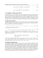
4. Robotic waveguide system
We designed a prototype of the robotic waveguide system to apply to a GE-PON optical
fiber line replacement according to the procedure described below.
An optical line length adjuster, shown in Photo 1, is installed along the detour line. The
adjuster is equipped with two retroreflectors, which directly face each other as shown in Fig.
6. A retroreflector consists of three plane mirrors, each of which is placed at right angles to
the other two. And it accurately reflects an incident beam in the opposite direction
regardless of its original direction, but with an offset distance. The vertex of the three
mirrors in the retroreflector is in the middle of a common perpendicular of the axes of the
incoming and outgoing beams as shown in Fig. 6. The number of reflections is determined
based on the retroreflector arrangement. A laser beam travels 10 times between the
retroreflectors in our prototype, and are introduced into the other optical fiber. Optical
pulses are transmitted through an optical fiber, divided into three wavelengths by
wavelength division multiplexing (WDM) couplers, and discharged separately into the air
from collimators. The focuses of a pair of collimators corresponding for a wavelength is best
tuned for the wavelength to achieve the minimum coupling loss. The collimators for
multiple wavelenghts are arranged to share the two retroreflectors as shown in Fig. 7.
The detour line between the retroreflectors consists of an FSO system [9]. The detour line
length can be easily adjusted by controlling the retroreflector interval with a resolution of
0.14 mm. Optical pulses travel n-times faster in the air than in an optical fiber, where n is the
refractive index of the optical fiber. Thus the optical line length adjuster lengthens/shortens
the corresponding optical fiber length, L, by k

x/n, where k,

x, n are the number of journeys
between the retroreflectors, the retroreflector interval variation, and the refractive index of
optical fiber, respectively. The FSO lengthens the optical line length up to L

0
.

Advances in Mechatronics

216

Photo 1. Free-space optics line length adjuster.


Fig. 6. Free-space optics line length adjuster.
x

xL




8
Retroreflecto
Collimato
SM
Guide
d
Retroreflector
vertex offset
View direction

Robotic Waveguide by Free Space Optics

217
L
0
= k

x
max
/ n, (5)
where

x
max
is the maximum range of the retroreflector interval variation. The maximum
range of our prototype,

x
max
, is around 0.3 m, the refractive index, n, of the optical fiber is
1.46, the number of journeys, k is 10, and the optical line span, L
0
, tuned by the adjuster is 2
m.


Fig. 7. Collimator arrangement for use of multiple wavelengths.


Fig. 8. FSO system with optical path length accumulation mechanism.
WDM
coupler





FSO
SW -0
SW -1
FS -1
Path #0
Path #1
L
0
2
L
0
3
L
0
FS
-
0
WIC2
WIC3
To WIC1
To detour line

Advances in Mechatronics

218
The limit of the adjustable range is a practical problem when this system is applied to

several kilometers of access network. Therefore, we employ optical line length
accumulators. The optical line length adjuster contains two optical paths, #0 and #1 as
shown in Fig. 1 or Fig. 8. An optical switch and an optical fiber selector are installed in each
path. Optical switches control the optical pulse flow. Each optical fiber selector is equipped
with various lengths of optical fiber, for example L
0
, 2L
0
and 3L
0
. The path length can be
discretely changed by choosing any one of them.
The optical line length adjuster can extend the detour line as much as required using the
following operation as shown in Fig. 9. First, the FSO system lengthens path #0 by L
0
by
gradually increasing the retroreflector interval. After the optical fiber selector has selected
an optical fiber of length L
0
, the active line is switched from path #0 to path #1. The FSO
system then returns to the origin, and the optical fiber selector selects an optical fiber of
length L
0
instead to keep the length of path #0 at L
0
. The FSO system increases the
retroreflector interval again to repeat the same operation. In this way the adjuster
accumulates spans extended by the FSO system. The scanning time of our prototype is 10
seconds, because the retroreflector operates at 30 mm/s.
The optical line length adjuster enables us to lengthen/shorten the detour line while

continuing to transmit optical signals.


Fig. 9. Time chart of operation for optical path length accumulation.
5. Experiments on optical line replacement
The optical line replacement procedure, shown in Fig. 10 where a 2x8 optical splitter is used
instead of a 2x2 splitter, is as follows:
1. A detour line is established between a WIC and a 2x8 optical splitter.
2. The detour line length is measured with a 1650 nm test light using an optical line length
measuring technique, and is adjusted to the same length as the regular line using an
optical line length adjusting technique. These techniques are described in the preceding
sections.
0
L
0
2L
0
T
T
2
T3
T
4
0
Time
Extended path length
Path #0
Path #1
Path extension
between WICs

2 and 3

Robotic Waveguide by Free Space Optics

219
3. Once the lengths of the two lines coincide, the transmission signals are also launched
into the detour line.
4. The regular line is cut and replaced with a new line, while the signals are being
transmitted through the detour line. A long-wavelength pass filter (LWPF) is
temporarily installed in the new line.
5. The test light measures the lengths of the new line and the detour line. The detour line
is adjusted to the new line while communications are maintained. The LWPF prevents
only the optical transmission pulses from traveling through the new line.
6. The LWPF is then removed and the transmission is duplicated. The detour line is finally
cut off.

(1) Set detour line.
(2) Adjust detour line to regular line.
(3) Multiplex optical signals.
Detour line
OLT
2
8
+
ONU
ONU
ONU
1650nmLD
OLT
2

8
+
ONU
ONU
ONU
1650nmLD
OLT
2
8
+
ONU
ONU
ONU
1650nmLD
Regular line
Optical line
length adjuster
WIC
Optical
splitter

(4) Cut regular line, and connect new line.
(5) Adjust detour line to new line.
(6) Cut off detour line.
OLT
2
8
+
ONU
ONU

ONU
1650nmLD
OLT
2
8
+
ONU
ONU
ONU
1650nmLD
OLT
2
8
+
ONU
ONU
ONU
1650nmLD
New line
LWPF

Fig. 10. Optical line replacement procedure.

Advances in Mechatronics

220
We investigated the tolerance of the multiplexed signal synchronicity in advance. The
transmission quality is observed by changing the difference between the duplicated line
lengths. The results show that the transmission linkage is maintained if the difference is
within 80 mm as with GE-PON. A multiplexed signal cannot be perceived as a single bit

when the duplicated line lengths have a larger gap for 1 Gbit/s transmission. Because these
characteristics depend on the periodic length of a transmission bit, the requirement is
assumed to be severe when the method is applied to higher-speed communication services.
Next, we constructed a prototype of the robotic waveguide system shown in Fig. 1, and
applied it to a 15 km GE-PON optical transmission line replacement. A 10 m optical fiber
extension was added to the transmission line, while optical signals were switched between
the duplicated lines during transmission.
Figure 11 shows the frame loss that occurred during optical line replacement, which we
measured with a SmartBit network performance analyzer. No frame loss was observed at
any switching stage if the difference between the duplicated line lengths was less than 80
mm. If the difference exceeded 80 mm, signal multiplexing caused frame loss in stages (a)
and (d). We confirmed that the optical signals can be completely switched between the
regular, detour, and new lines on condition that the line length is adjusted with sufficient
accuracy.
The experimental results proved that our proposed system successfully relocated an in-
service broadband network without any service interruption.


Fig. 11. Frame loss while replacing transmission line according to the procedure; (a)
Multiplex signals of current line and detour line, (b) Cut current line, (c) Extend detour line,
(d) Multiplex signals of detour line and new line, (e) Cut off detour line.
6. Conclusion
We proposed a new switching method for in-service optical transmission lines that transfers
live optical signals. The method exchanges optical fibers instead of using electric apparatus
Optical line replacement procedure
Frame loss (%)
:0
:50
:80
:120

Line
difference
0
2
4
6
8
10
(a) (b) (c) (d) (e)

Robotic Waveguide by Free Space Optics

221
to control transmission speed. The robotic waveguide system is designed to apply to
duplicated optical lines. An optical line length adjuster, designed based on an FSO system,
continuously lengthened the optical line up to 100 m with a resolution of 0.1 mm. An optical
line length measurement technique successfully evaluated the difference in length between
the duplicated lines from 100 m to 10 mm. An interferometry measurement distinguished
the difference between line lengths to an accuracy of better than 10 mm by analyzing
interfering waveforms created by chirped laser pulses. We applied this system to a 15 km
GE-PON network and succeeded in replacing the communication lines without inducing
any frame loss.
7. References
Tanaka, K.; Zaima, M.; Tachikura, M. & Nakamura, M. (2002). Downsized and
enhanced optical fiber cable transfer splicing system, Proceedings of 51
st
IWCS,
2002
Azuma, Y.; Tanaka, K. ; Yoshida, K. ; Katayama, K.; Tsujimura, T.; & Shimizu, M. (2008).
Basic investigation of new transfer method for optical access line, IEICE Technical

Report Japan, OFT2008-52, pp. 27-31, 2008
Tanaka, K.; Tsujimura, T.; Yoshida, K. ; Katayama, K.; & Azuma, Y. (2009). Frame-loss-free
Line Switching Method for In-service Optical Access Network using Interferometry
Line Length Measurement, OFC2009, paper PDPD6, 2009
Tanaka, K.; Tsujimura, T.; Yoshida, K. ; Katayama, K.; Azuma, Y. M.; & Shimizu, M. (2010).
Frame-Loss-Free Optical Line Switching System for In-Service Optical Network, J.
Lightw. Technol., Vol.28, No.4, pp. 539-546, 2010.
Tsujimura, T.; Tanaka, K.; Yoshida, K. ; Katayama, K.; & Azuma, Y. (2009). Infallible Layer-
one Protection Switching Technique for Optical Fiber Network, Proceedings of 14th
European Conference on Networks and Optical Communications/ 4th Conference on
Optical Cabling and Infrastructure, 2009
Saunders, R.; King, J. & Hardcastle, I. (1994). Wideband chirp measurement technique
for high bit rate sources, Electronics Letters, Vol.30, No.16, pp. 1336-1338,
1994.
Cao, S. & Cartledge, J. (2002). Measurement-Based Method for Characterizing the Intensity
and Phase Modulation Properties of SOA-MZI Wavelength Converters, IEEE
Photonics Technology Letters, Vol.14, No.11, pp. 1578-1580, 2002
Torregrosa, A. et al., Return-to-Zero Pulse Generators Using Overdriven Amplitude
Modulators at One Fourth of the Data Rate, IEEE Photonics Technology Letters,
Vol.19, No.22, pp. 1837-1839, 2007
Fukada, Y.; Suzuki, K.; Nakamura, H.; Yoshimoto, N. & Tsubokawa, M. (2008). First
demonstration of fast automatic-gain-control (AGC) PDFA for amplifying burst-
mode PON upstream signal, ECOC2008, paper WE.2.F.4, 2008.
Yoshida, K.; Tsujimura, T. & Kurashima, T. (2008). Seamless transmission between single-
mode optical fibers using free space optics system, SICE Annual Conference, pp.
2219-2222, 2008

Advances in Mechatronics

222

Yoshida, K. & Tsujimura, T. (2010). Seamless Transmission Between Single-mode Optical
Fibers Using Free Space Optics System, SICE J. Contr. Measure. Syst. Integr. (JCMSI),
Vol.3, No.2, pp.94-100, 2010.
11
Surface Reconstruction of Defective Point
Clouds Based on Dual Off-Set
Gradient Functions
Kun Mo
1
and Zhoupin Yin
2

1
Dongfang Electric Corporation, Research & Develop Centre, Intelligent Equipment &
Control Technology Institute
2
State Key Laboratory of Digital Manufacturing Equipment and Technology
Huazhong University of Science and Technology
China
1. Introduction
Surface reconstruction is an interesting and challenging task in extensively applied fields
including rapid prototype manufacturing, computer vision, virtual reality and computer
aided design (CAD). A typical reconstruction procedure begins with scanning, in which the
point data are sampled from physical objects by digitizing measurement systems (such as
laser-range scanners and hand-held digitizers). And then, the point data are generated as a
smooth, water-tight and proper resulting surface by a suitable reconstruction method. In
industry the most difficulty comes from the defective samples that are subject to the noise,
holes and overlapping regions. The defective samples are often unavoidable due to the
sampling inaccuracy, scan mis-registration and accessibility constraints of scanning device.
They often make most existing reconstruction methods not practical for engineering

application because the oriented or neighbour information of points, which the most
methods are highly based on, are hard to evaluate. For instance, many methods rely on
consistent normals, or pose the demand on triangular meshes generated from point data.
However, the holes and overlapping samples confuse the point’s neighbour relationship,
some jagged, self-intersect regions could exist in the corresponding triangular mesh or the
estimation of consistent normals becomes an ill-posed problem. Only a few methods need
not such specific information, but they have to resort to some complex or time-consuming
steps, like re-sampling, distance-computing, mesh-smooth or deformable models. Even if
these methods can generate a water-tight resulting surface, the reasonableness of fitting
overlapping samples and holes is not guaranteed. In fact, such issues, especially “bad-
scanning” data, often lead long scanning time, massive manual work and poor model
quality.
Given these challenges, this paper propose a novel surface reconstruction method that takes
as input defective point clouds without any specific information and output a smooth and
water-tight surface. The main idea is that (1) this technique is based on implicit function,
because implicit reconstruction is convenient to guarantee a water-tight result; (2) the
approach is indirect, two off-set surfaces are generated to best fit the point clouds instead of
direct approximation. As shown in Fig.1 (1D situation for simple expression), the point

Advances in Mechatronics

224
clouds are represented as origin of coordinates (Fig. 1 (a)). The space is divided into inside
part (positive axis in Fig. 1 (a)) and outside part (negative axis in Fig. 1 (a)). If the point
clouds are defective, it is very hard to reconstruct final implicit function with w -width(real
line in Fig.1 (b)) directly, including reducing noise, filling holes and merging overlapping
samples. Therefore, this method constructs dual off-set functions to approximate the inner
and outer level set of the final implicit surface (real lines in Fig.1 (c)). The dual water-tight
surfaces form a minimal crust surrounding the point data. Based on the dual relative
functions, a novel energy function is defined. By minimizing the energy function, the

resulting surface (dash dot line in Fig.1 (c)) is finally obtained and visualized.

inside
outside
Point clouds
inside
outside
Point clouds

inside
outside
w-width
inside
outside
w-width
inside
function
outside
function
result
surface
inside
function
outside
function
result
surface

(a) (b) (c)
Fig. 1. The main idea of this method: (a) Point clouds. (b) Implicit resulting surface. (c) Off-

set functions and resulting surface.
The dual relative functions are built on volumetric grids by extending some sophisticated
2D grey image processing algorithms into 3D space, including morphology operation and
weighted vector median filter algorithm. The method needs not any specific information
and also has the advantages that (1) the implementation needs not time-consuming steps,
like computing distances between each point which is performed normally by most existing
methods; (2) the dual gradient functions provide global constrains to the resulting surface,
the holes could be filled smoothly and the overlapping samples could be fitted much
reasonably. (3) the method can successfully construct “bad-scanning” point data which
could not be handled by many methods. The reminder of the paper is organized as follows,
after the previous works are reviewed and compared in section 2, the process and details of
this method is described in section 3. To demonstrate the effectiveness, extensive numerical
implementations are discussed in section 4. Finally, the conclusion and future work is
summarized in section 5.
2. Related work
The previous algorithms of surface reconstruction can be generally classified into two
categories: explicit methods and implicit methods. Most explicit methods employ Delaunay-
triangulation or Voronoi diagrams, like alpha shapes (Edelsbrunner & Mücke 1994), crust
method (Nina et al. 1998), triangular-sculpting (Jean-Daniel 1984), mesh growing (Li et al.
2009) and their developed version(Veltkamp 1995; Baining et al. 1997; Attali 1998; Amenta et
al. 2000; Amenta et al. 2001; Yang et al. 2009). But the noise and overlapping samples could
make the resulting surface jagged. Smoothing (Ravikrishna et al. 2004), refitting (e.g.
(Chandrajit et al. 1995; Shen et al. 2005; Shen et al. 2009)) or blending (LA Piegl 1997) of
subsequent processing are required.
In contrast, the implicit methods are much efficacious to infer topology of points, blend
surface primitives, tolerate noise, and fill holes automatically. A popular algorithm is based

Surface Reconstruction of Defective Point Clouds Based on Dual Off-Set Gradient Functions

225

on blending locally fitted implicit primitives, such as Radial basis functions (RBF) method
(Carr et al. 2001; Greg & James 2002), multi-level partition of unity (MPU) method (Yutaka
et al. 2003), products of univariate B-splines (Song & Jüttler 2009) and tri-cubic B-spline basis
functions (Esteve et al. 2008) on voxelization. However they either need the consistent
normals as aided information or the point clouds with fewer defective samples. The local
primitives also include polynomial of point set surface (Alexa et al. 2001; Gael & Markus
2007) with moving least squares (MLS) approximation. MLS methods have to employ
normal computation and projection operators, which could lead to low efficiency and need
certain extra procedure to improve (Anders & Marc 2003; Marc & Anders 2004). Some
methods need pre- or post-processing, like oriented estimation (Vanco & Brunnett 2004;
David & Guido 2005), smooth operation (e.g. (Yukie et al. 2009)) or holes filling. For
instance, the method proposed in (Davis et al. 2002) uses diffusion to fill holes on
reconstructed surfaces. The approach essentially solves the homogeneous partial differential
equation (PDE) given boundary conditions to create an implicit surface spanning
boundaries. Poisson method (Michael et al. 2006) is also a PDE-based reconstruction
algorithm with oriented point clouds. Several approaches use combinatorial structures, such
as signed distance function and Voronoi diagram as (Boissonnat & Cazals 2002) (Hybrid
method). But the normal information of point clouds is still required.
Only a few methods could demand little restriction on point data. Hoppe’s method (Hoppe
et al. 1992) is a typical method of this category. It creates the object surface by locally fitting
planes to generate a signed distance function and triangulate its zero-level set. The signed
distance function can also be cumulated into volumetric grids as proposed in (Brian & Marc
1996). But the two methods are troubled by the noisy or sparse data, which make the
connection relationship of these regions hard to confirm. The method proposed in (Alliez et
al. 2007) employs Voronoi diagram to estimate the un-consistent normals and solves a
generalized eigenvalue problem to construct resulting surface. However, it has to suffer
from low computation efficiency. Level set method (Zhao et al. 2000), a typical deformable
models, reconstructs the surface by solving corresponding level set equation defined on
point data. It is a time-consuming method since it requires a process of re-initialization and
needs updating all the nodes of compute grids in very time step. The reconstruction method

also employ voting algorithm (Xie et al. 2004) to cluster points into local groups, which are
then blended to produce a signed distance field using the modified Shepard’s method. But it
needs to compute the medial axis transformation and perform an active contour growing
process, like deformable models. The methods in (Esteve et al. 2005) proposes DMS
operation on volumetric grids to fill holes by detecting the incursions to the interior of the
surface and approximates them with a bounded maximum distance. It is an improvement of
(Song & Jüttler 2009), but a post process has to be introduced to the low density data zones.
The typical implicit methods mentioned above are summarized in Table 1 with four respects
that whether the methods need specific information and have the effectiveness of reducing
noise, filling holes and merging overlapping samples. Although all the implicit methods can
guarantee water-tight results that the holes could be filled, some methods (like Level set
method) could not fill holes smoothly. Many methods have certain low efficient steps, like
solving density matrix equation (e.g. RBF), projection procedure (e.g. MLS) and compute the
distance function among all the point clouds for neighbor information. All the methods can
reduce noise, but the effectiveness is not the same. For instance, MPU and Hoppe’s method
could be influenced by noise more than others, if the noise is too much the resulting surface
is still not smooth. All the methods do not address how to merge overlapping samples,
especially the “bad-scanning” points, which is a common problem in practice.

Advances in Mechatronics

226
Method name
Specific
information
Reduce
noise
Fill holes
Merge overlapping
samples

RBF (Carr et al. 2001; Greg
& James 2002)
Yes Yes Yes
——
MPU (Yutaka et al. 2003) Yes Yes Yes
——
MLS (Marc et al. 2001;
Gael & Markus 2007)
No Yes Yes
——
Poisson method (Michael
et al. 2006)
Yes Yes Yes
——
Hybrid method
(Boissonnat & Cazals 2002)

Yes Yes Yes
——
Hoppe’s method (Hoppe
et al. 1992)
No Yes Yes
——
Voronoi method (Alliez et
al. 2007)
No Yes Yes
——
Level set method (Zhao et
al. 2000)
No Yes Yes

——
Voting algorithm (Xie et
al. 2004)
No Yes Yes
——
DMS method (Esteve et al.
2005)
No Yes Yes
——
This method No Yes Yes Yes
Table 1. Comparison between this method and typical implicit methods.
Rather than constructing final surface directly, it is much easier to confirm the off-set
surfaces of point clouds. Some methods have focused on the respect, like duplex fitting
method (Liu & Wang 2009) or dual-RBF method (Lin et al. 2009). But they need the
consistent normals for accurately fitting. Recently, some robust and efficient methods in
other research areas (like image processing (Peng & Loftus 1998; Peng & Loftus 2001) and
statistics (Roca-Pardinas et al. 2008)) have been introduced in reverse engineering. Inspired
by the two ideas, this paper describes a novel reconstruction method using the dual off-set
surface by extending morphology operation and weighted vector median filter algrithms.
The comparison between this method and typical implicit methods is added in Table 1. This
method provides a convenient and efficient manner for reconstruction and addresses the
issues of overlapping points and “bad-scanning” samples.
3. Method description
The main process of the proposed method is illustrated in Fig.2. Let
12
{,, }
m
p
ppP
represent defective point clouds (black points in Fig.2) sampled from a real object surface

S (black line in Fig.2). The goal of this method is to reconstruct an implicit
function
() x whose zero level set approximates S reasonably. The general intermediate step
is to approximate



, which denote the offset surfaces to S with slight distance  . Finally,
() x is generated by blending



according to a minimal model. The mathematic
description can be defined as follow: given the position coordinates of discrete point
sets
P around 3D local region V , find an implicit function

that satisfy,

Surface Reconstruction of Defective Point Clouds Based on Dual Off-Set Gradient Functions

227

() 0 for
() 0 for
() 0 for
 


 






xxV
xxV
xxΓ V
(1)
by approximating the offset function
in
f



 and
out
f



 .

Γ V in Eq. (1)represents the
interface of the region
V
.
In the first step,
out
f

and
in
f
are constructed on volumetric grids respectively (represented as
two red lines in Fig.2 (b)). The dual functions are water-tight and guarantee a minimal
narrowband surrounding the point clouds. This step is accomplished by the morphology
operation, a powerful theory in image processing (Maragos et al. 1996). In the second step,
by blurring the boundary of
out
f and
in
f , two monotonic functions are obtained and
transformed as gradient fields (arrows in Fig. 2 (c)). This paper extends weighted vector
median filter algorithm to reduce the noise influence. In the third step, the surface
reconstruction problem is formulated as solving a minimal energy model by blending the
dual gradient fields (arrows in Fig. 2 (d)). By deriving and solving the corresponding Euler-
Lagrange equation, the implicit resulting function is obtained. Finally, the reconstructed
surface is extracted by marching cube method (William & Harvey 1987) and visualized
(dashed line in Fig. 2 (e)).


(a) (b) (c) (d) (e)
Fig. 2. The main process of the proposed method.
3.1 Generate off-set functions
The point data are first need divide into volumetric grids (voxelization). A best voxelization
is that the size of voxel cooperates with the data density, where one grid only contains one
point. As shown in Fig. 3, the black points represent defective points and the real line
represents the reasonable resulting surface. If the point clouds are uniform, the voxel-
building step is immediate. In industry, the uniform samples are common data because the
original scanning data are numerous, a regular sampling for reduction are often needed

before reconstruction. If the point data have a very irregular sampling density, the ratio,
number of voxels which contain two or more points divided by the total number, should be
calculated. If the valve is too high, the size of the volumetric grids is re-calculated by
decreasing the length of grids. The most difficulty is how to guarantee off-surface,
in
f
and
out
f
, water-tight. It needs determining the inside/outside of the grids near defective
samples, especially holes and overlapping regions (circles in Fig.3 (a)). This method extends
the basic operations of mathematical morphology, dilation and erosion, to confirm the sign
of
in
f and
out
f near the holes and overlapping samples (dash dot line in Fig.3 (b)).

Advances in Mechatronics

228
resulting surface

(a) (b)
Fig. 3. The main idea of constructing dual off-set functions. (a) Defective point clouds. (b)
off-set surface and resulting surface.
To express simply, 2D uniform point clouds of arbitrary shape are designed (Fig.4 (a)). This
shape contains lines, fillets and free curves according to the practical products. Some
random noise, overlapping regions and holes are added. Fig.4 (b) shows the voxelization
results. The node (white rectangles) of the grids within points (black points) is labeled as

value 1 and other nodes are labeled as value -1. The dilation operation of morphology is
then used to construct a rough crust (as shown in Fig. 4 (d)). Let
(,,)xyzF denote the point
image of voxelization and
B denote structuring element. Dilation of the image (,,)xyzF by an
element
B is denoted by



(,,) max ( , , ) (,, )x
y
zxu
y
vz w uvw FB F B (1)
The best choice of B should preserve the shape of point clouds and perform dilation with
less times. According to the research (Maragos et al. 1996), a disk shape (as shown in Fig.4
(c)) in 3D space is a good choice. If
B is a rectangle or sphere shape, some shape details may
be blurred. The structuring element size should be little larger than the noise distribution. If
error of noise is defined as
r

, the length of B should be set as

() int( )
r
l
h


B
(2)
where
()l B represents the length of B , h denotes the grid size according to the density of
points,
int( ) is rounded down function. For instance, if the random noise
with
2
(0,0.1 )
r
N  is added in points and the grid size is defined as 0.05mm , the structuring
element size should be more than 2. If the size of
B is too large, although the dilation times is
less, the shape of points could be blurred. A suitable selection is given by

int( ) ( ) int(3 )
rr
l
hh



B
(3)
In this paper, it is generally set as median size 3 3 3

 (Fig. 4 (c)), if the point clouds are
much dense with little noise, the size can be smaller.
By the close crust, the inside and outside of the point data can be roughly separated. The
inside part is then filled (see Fig. 4 (e)) by a simple flood-fill algorithm. It starts at a node

(E.g. the middle gird node) known to be inside, those nodes accessible from initial node are
labeled “inside”, and the remaining nodes are labeled “outside”. Each node of resulting
image is therefore classified as lying inside the object (value 1) and outside/on the object
(value -1). When sparse samples or large holes exist, the dilation should be executed for
several times until a water-tight crust is constructed. The flood-fill step can check if the crust