Aeronautics and Astronautics Part 5 doc

Physico - Chemical Modelling in Nonequilibrium Hypersonic Flow Around Blunt Bodies 25
X/R
Temperatures, K
-0.12 -0.1 -0.08 -0.06 -0.04 -0.02 0
0
2000
4000
6000
8000
10000
12000
T
T
T
T
v
v
e
O2
N2
without correction
with correction
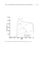
Fig. 9. Temperature along stagnation line with weakly ionized gas; M
∞
= 18
149
Physico - Chemical Modelling in Nonequilibrium Hypersonic Flow Around Blunt Bodies
26 Aeronautics and Astronautics
X/R
-0.15 -0.125 -0.1 -0.075 -0.05 -0.025 0
0

2000
4000
6000
8000
10000
12000
14000
16000
18000
20000
22000
Park 93
Gardiner
Moss
Modif. Dunn & Kang
With Gupta curve fit constants and Park CVD
T[°K]
T
T
v
N
M =25.9
∞
2
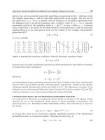
Fig. 10. Temperature profile with Gupta curve fit constants, M
∞
=25.9
150
Aeronautics and Astronautics
Physico - Chemical Modelling in Nonequilibrium Hypersonic Flow Around Blunt Bodies 27

θ
0 10 20 30 40 50 60 70 80 90
0
0.5
1
1.5
2
2.5
3
Park (93)
Gardiner
Moss
Dunn & Kang
With Park CVD
With Hansen CVD
Q(MW/m)
w
2
With Gupta Curve fit Constants
Modif. Dunn & Kang
M =25.9
∞
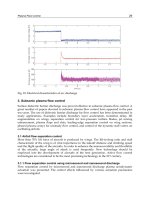
Fig. 11. Stagnation heat flux, M
∞
=25.9
151
Physico - Chemical Modelling in Nonequilibrium Hypersonic Flow Around Blunt Bodies
28 Aeronautics and Astronautics
X/R
Temperatures, K

-0.12 -0.1 -0.08 -0.06 -0.04 -0.02 0
0
4000
8000
12000
16000
20000
T
T
T
T
V
V
e
O2
N2
Fig. 12. Temperatures distribution along the stagnation line, M
∞
=23.9
152
Aeronautics and Astronautics
Physico - Chemical Modelling in Nonequilibrium Hypersonic Flow Around Blunt Bodies 29
X/R
Ne
0 1 2 3 4 5 6 7 8
10
9
10
10
10

11
10
12
10
13
10
14
Mach=23,9; H=61 Km
Experiment, H=61 Km
Δ
Δ
Δ
Δ
Ο
Ο
Ο
Ο
Mach=25,9; H=71 Km
Experiment, H=71 Km
Δ
Ο
Fig. 13. Comparison with experiment of the peak of electron number density following the
axial distance
153
Physico - Chemical Modelling in Nonequilibrium Hypersonic Flow Around Blunt Bodies
30 Aeronautics and Astronautics
Dunn & Kang
Dunn & Kang with Gupta
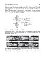
Fig. 14. Dunn and Kang, and Modified Dunn and Kang Interferograms computed
Fig. 15. Fringe patterns on 1 in diameter cylinder with Park(93) model and Exact equilibrium

constant
154
Aeronautics and Astronautics
Physico - Chemical Modelling in Nonequilibrium Hypersonic Flow Around Blunt Bodies 31
Fig. 16. Fringe patterns on 1 in diameter cylinder with Gardiner model and Exact
equilibrium constant
155
Physico - Chemical Modelling in Nonequilibrium Hypersonic Flow Around Blunt Bodies
32 Aeronautics and Astronautics
Chemistry of Gardiner
Chemistry of Park
15°
60°
M
∞
=9
Gardiner
Park
S/L
P/P
0 0.5 1 1.5 2
0
100
200
300
400
500
∞
Chemistry of Gardiner
Chemistry of Park

θ =15°
θ =60°
∞
Μ=9
1
2
Fig. 17. Effect of chemical kinetics: a) Contours Mach number b) Surface pressure
6. Conclusion
The hypersonic flow past blunt bodies with thermo-chemical nonequilibrium were
numerically simulated. The dependence of solutions on available chemical models, allowing
to assess the accuracy of finite rate chemical processes has been examined. The present results
were successfully validated with the theoretical and experimental work for shock-standoff
distances, stagnation point heat transfer and interferograms of the flow. Although all model
describe the essential aspects of the nonequilibrium zone behind the shock, they are not
accurate for the evaluation of the aerothermodynamic parameters. A comparative study of
various kinetic air models is carried out to identify the reliable models for applications with a
wide range of Mach number.
The present study has shown that the prediction of hypersonic flowfield structures, shock
shapes, and vehicle surface properties are very sensitive to the choice of the kinetic model.
The large dispersion in the wall heat flux reaches 60 % as observed in the RAM-CII case. The
manner in which the backward reaction rates are computed is quite important as indicated
by the interferograms that were obtained. The model of Park (93) gives a better prediction
of hypersonic flowfield around blunt bodies. Park(93) is identify as the model for hypersonic
flow around blunt bodies with a confidence acceptable to a wide range of Mach number. There
is also great sensitivity to the choice of chemical kinetics in flowfield around double-wedge.
More numerical simulations compared with experiments need to be conducted to improve
the knowledge of the thermochemical model of air flow around double-wedge.
7. References
[1] Park, C. (1990). Nonequilibrium Hypersonic Aerothermodynamics. New York, Wiley.
[2] Gupta, R. N., Yos, J. M., Thompson, R. A., and Lee, K. P. (1990). A Review of Reaction

Rates and Thermodynamic and Transport Properties for an 11-Species Air Model for
Chemical and Thermal Nonequilibrium Calculations to 30 000K", NASA RP-1232.
[3] Vincenti, W. G., Jr.Kruger, C. H. (1965). Introduction to physical Gas Dynamics. Krieger, FL.
[4] Gardiner, W. C. (1984). Combustion Chemistry, Springer-Verlag, Berlin.
156
Aeronautics and Astronautics
Physico - Chemical Modelling in Nonequilibrium Hypersonic Flow Around Blunt Bodies 33
[5] Shinn, J. L., Moss, J. N., Simmonds, A. L. (1982). Viscous Shock Layer Heating Analysis
for the Shuttle Winward Plane Finite Recombination Rates, AIAA 82-0842.
[6] Dunn,M. G., Kang, S. W. (1973). Theoretical and Experimental Studies of re-entry Plasma,
NASA CR-2232.
[7] Park, C. (1993). Review of Chemical-Kinetic Problems of Future NASA Mission, I: Earth
Entries", Journal of Thermophysics and Heat Transfer. Vol. 7, No. 3, pp. 385-398.
[8] Hansen, C. F. (1993). Vibrational Nonequilibrium Effect on Diatomic Dissociation Rates".
AIAA Journal, Vol. 31, No. 11, pp. 2047-2051.
[9] Macrossan, N. M. (1990). Hypervelocity flow of dissociating nitrogen donwnstream of a
blunt nose. Journal of Fluid Mechanics, Vol. 27, pp. 167-202.
[10] Josyula, E. (2001). Oxygen atoms effect on vibrational relaxation of nitrogen in blunt body
flows. Journal of Thermophysics and Heat Transfer, Vol. 15, No. 1, pp. 106-115.
[11] Peter, A. G. and Roop, N. G. and Judy, L. S. (1989). Conservation Equation and Physical
Models for Hypersonic Air flows in Thermal and Chemical Nonequilibrium. NASA TP
2867.
[12] Knab, O. and Fruaudf, HH. and Messerschmid, EW. (1995). Theory and validation of
the the physically consistent coupled vibration-chemistry-vibration model. J. Thermophys
Heat Transfer,nˇr9, Vol.2, pp.219-226.
[13] Tchuen G., Burtschell Y., and Zeitoun E. D. (2008). Computation of non-equilibrium
hypersonic flow with Artificially Upstream Flux vector Splitting (AUFS) schemes.
International Journal of Computational Fluid Dynamics, Vol. 22, Nˇr4, pp. 209 - 220.
[14] Tchuen G., and Zeitoun D. E. (2008). Computation of thermo-chemical nonequilibrium
weakly ionized air flow over sphere cones. International journal of heat and fluid flow,

Vol.29, Issue 5, pp.1393 - 1401.
[15] Tchuen G., and Zeitoun D. E. (2009). Effects of chemistry in nonequilibrium hypersonic
flow around blunt bodies. Journal of Thermophysics and Heat Transfer, Vol. 23, Nˇr3,
pp.433-442.
[16] Burtschell Y., Tchuen G., and Zeitoun E. D. (2010). H2 injection and combustion in a Mach
5 air inlet through a Viscous Mach Interaction. European Journal of Mechanics B/fluid,Vol.
29, Issue 5, pp. 351-356.
[17] Lee Jong-Hun. (1985). Basic Governing Equations for the Flight Regimes of Aeroassisted
Orbital Transfer Vehicles. Thermal Design of Aeroassisted Orbital Transfer Vehicles, H.
F. Nelson, ed., Volume 96 of progress in Astronautics and Aeronautics, American Inst. of
Aeronautics and Astronautics, Vol. 96, pp. 3-53.
[18] Appleton, J. P. and Bray, K. N. C. (1964). The Conservation Equations for a
Nonequilibrium Plasma. J. Fluid Mech. Vol. 20, No. 4, pp. 659-672.
[19] Tchuen, G., Burtschell, Y., and Zeitoun, E. D., 2005. Numerical study of nonequilibrium
weakly ionized air flow past blunt body. Int. J. of Numerical Methods for heat and fluid
flow, 15 (6), 588 - 610.
[20] Blottner, F. G., Johnson, M., and Ellis, M., 1971. Chemically Reacting Viscous Flow
Program for Multi-Component Gas Mixtures. Sandia Laboratories, Albuquerque, NM,
Rept. Sc-RR-70-754.
[21] Wilke, C. R., 1950. A viscosity Equation for Gas Mixture. J. of Chem. Phys. 18 (4), 517-519.
[22] Ramsaw JD., and Chang CH., 1993. Ambipolar diffusion in two temperature
multicomponent plasma. Plasma Chem Plasma process. 13 (3), 489-498.
157
Physico - Chemical Modelling in Nonequilibrium Hypersonic Flow Around Blunt Bodies
34 Aeronautics and Astronautics
[23] Masson, E. A., and Monchick, 1962. Heat Conductivity of Polyatomic and Polar Gases.
The Journal of Chemical. 36 (6), 1622-1640.
[24] Ahtye, W. F., 1972. Thermal Conductivity in Vibrationnally Excited Gases. Journal of
Chemical Physics, 57, 5542-5555.
[25] Candler, G. V., and MacCormarck, R. W., 1991. Computation of weakly ionized

hypersonic flows in thermochemical nonequilibrium. Journal of Thermophysics and heat
transfer, 5 (3), 266-273.
[26] Taylor R., Camac, M., and Feinberg, M., 1967. Measurement of vibration-vibration
coupling in gas mixtures, In Proceeding of the 11th Intenational Symposium on
combustion, Pittsburg, PA, 49-65.
[27] Sharma, S. P., Huo, W. M., and Park, C., 1988. The Rate Parameters for Coupled
Vibration-Dissociation in a Generalized SSH Approximation Flows. AIAA-88-2714.
[28] Shatalov, O. P., and Losev, S. A., "Modeling of diatomic molecules dissociation under
quasistationary conditions", AIAA 97-2579, 1997.
[29] Roe, P., 1983. Approximate Riemann Solvers, Parameters vectors and difference schemes.
Journal of Computational Physics, Vol. 43, 357-372.
[30] Lobb, K., "Experimental measurement of shock detachment distance on sphere fired in
air at hypervelocities", in The High Temperature Aspect of Hypersonic Flow. ed. Nelson W.
C., Pergamon Press, Macmillan Co., New York, 1964.
[31] Rose, P. H., Stankevics, J. O., "Stagnation-Point Heat Transfer Measurements in Partially
Ionized Air". AIAA Journal, Vol. 1, No. 12, 1963, pp. 2752-2763.
[32] Hornung, H. G., "Non-equilibrium dissociating nitrogen flow over spheres and circular
cylinders". Journal of Fluid Mechanics, Vol. 53, 1972, pp. 149-176.
[33] Joly, V., Coquel, F., Marmignon, C., Aretz, W., Metz, S., and Wilhelmi, H., "Numerical
modelling of heat transfer and relaxation in nonequilibrium air at hypersonic speeds", La
Recherche Aérospatiale, Vol.3, 1994, pp. 219-234.
[34] Séror, S., Schall, E., and Zeitoun, E. D., "Comparison between coupled euler/defect
boundary-layer and navier-stokes computations for nonequilibrium hypersonic flows,
Computers & Fluids, Vol.27, 1998, pp. 381-406.
[35] Fay, J. A., Riddell, F. R., "Theory of stagnation point heat transfer in dissociated air". J.
Aero. Sciences, Vol. 25, 1958, pp. 73-85.
[36] Walpot, L. M., "Development and Application of a Hypersonic Flow Solver". PhD thesis,
TU Delft, 2002.
[37] Soubrié, T., Rouzaud, O., Zeitoun, E. D., "Computation of weakly multi-ionized gases for
atmospheric entry using an extended Roe scheme". ECCOMAS, Jyväskylä, 2004.

[38] Candler, V. G., MacCormack, W. R., "The computation of hypersonic ionized flows in
chemical and thermal nonequilibrium". AIAA 88-0511, 1988.
158
Aeronautics and Astronautics
0
A Frequency-Domain Linearized Euler Model
for Noise Radiation
Andrea Iob, Roberto Della Ratta Rinaldi and Renzo Arina
Politecnico di Torino, DIASP, 10129 Torino
Italy
1. Introduction
Aeroacoustics is the branch of Fluid Mechanics studying the mechanism of generation
of noise by fluid motions and its propagation. The noise generation is associated with
turbulent and unsteady vortical flows, including the effects of any solid boundary in the flow.
Experimental studies in this field are very difficult, requiring anechoic wind tunnels and very
sensitive instruments able to capture high frequency, low amplitude, pressure fluctuations.
Computational Aeroacoustics (CAA) can be a powerful tool to simulate the aerodynamic
noise associated to complex turbulent flow fields. As sound production represents only a
very minute fraction of the energy associated to the flow motion, CAA methods for acoustic
propagation have to be more accurate compared to the solution schemes normally used in
Computational Fluid Dynamics (CFD).
A direct approach to aeroacoustic problems would imply to solve numerically the full
Navier-Stokes equations for three-dimensional, unsteady, compressible flows. Sound
would then be that part of the flow field which dominates at large distances from the
region characterized by intense hydrodynamic fluctuations, propagating at the local sound
speed. The direct noise simulation is hardly achievable in practice, except for very simple
configurations of academic interest, and in a limited region of space. Even if the small
amplitude of the fluctuations allow a linearization, the equations of acoustic disturbances
on an arbitrary base flow are very complicated and their solution is not straightforward.
To solve aeroacoustic problems of practical interest some simplifying approximations are

necessary. One way to obtain realistic solutions is provided by the hybrid approach. It
decouples the computation of the flow field from the computation of the acoustic field. When
using a hybrid method the aeroacoustic problem is solved in two steps: in the first step, the
hydrodynamic flow field is solved using a CFD method, then the noise sources are identified
and the acoustic field is obtained. Extraction of noise sources from the fluid dynamic field
can be done using an aeroacoustic theory such as the Lighthill’s analogy [Crighton (1975);
Goldstein (1976)]. A hybrid approach is based on the fundamental assumption that there is
a one-way coupling of mean flow and sound, i.e., the unsteady mean flow generates sound
and modifies its propagation, but sound waves do not affect the mean flow in any significant
way. This assumption is not so restrictive, because acoustic feedback is possible only when
the mechanical energy in the unsteady mean flow is weak enough to be influenced by acoustic
disturbances. This occurs principally in the vicinity of a starting point for flow instability (for
instance, upstream edges of cavities or initial areas of shear layers). Since the fluid-dynamic
6
2 Will-be-set-by-IN-TECH
field and the acoustic field are computed separately, numerical accuracy for the mean flow
simulations used as an input of hybrid methods is less critical than in direct computation.
Simpler, more flexible and lower-resolution schemes are applicable provided that numerical
dissipation is carefully controlled to prevent the artificial damping of high-frequency source
components. Incompressible flow solutions can be adequate for evaluating acoustic source
terms based on the low Mach numbers approximation. Time-accurate turbulence simulation
approaches such as DNS, LES, DES and unsteady RANS methods can be used to compute the
space-time history of the flow field, from which acoustic sources are extracted. Because of the
high computational cost of the time-accurate simulations, there have been efforts to use steady
RANS calculations in conjunction with a statistical model to generate the turbulent acoustic
terms.
Once the acoustics sources have been evaluated, the generated noise has to be propagated
in the surrounding region with linearized propagation models. The main focus of the present
chapter is the description of a computational method for noise propagation in turbomachinery
applications. In the next Section a linearized model is presented. Section 3 describes the

numerical algorithm based on a Discontinuous Galerkin approximation on unstructured
grids, and in Section 4 several applications are presented.
2. Governing equations
In principle the propagation of acoustic waves could be directly studied using the equations of
the fluid motion, i.e. the Navier Stokes equations. However, it is possible to introduce some
approximations in the Navier Stokes equations in order to obtain equations more suitable
for aeroacoustics. At frequencies of most practical interest, viscous effects are negligible in
the acoustic field because the pressure represents a far greater stress field than the viscous
stresses. Moreover, these disturbances are always small, also for very loudly acoustic waves.
The threshold of pain, i.e. the maximum Sound Pressure Level (SPL) which a human can
endure for a very short period of time without the risk of permanent ear damage, is equal to
140 dB, which corresponds to pressure fluctuations of amplitude equal to
A
=
√
2p
ref
10
(
SPL/20
)
≈ 90 Pa, (1)
where p
ref
is the reference pressure corresponding to the threshold of hearing at 1 kHz for a
typical human hear. For sound propagating in gases it is equal to p
ref
= 2 × 10
−5
Pa. The

atmospheric pressure of the standard air is equal to p
0
= 101325 Pa, which is 10
3
greater
than the pressure variation associated with an acoustic wave at the threshold of pain, i.e.,
p

/p
0
= O

10
−3

, where the superscript
(
.
)

denotes acoustic quantities and the subscript
(
.
)
0
denotes mean flow quantities. The corresponding density fluctuations of a progressive
plane wave are
ρ

ρ

0
=
p

ρ
0
c
2
0
, (2)
also of the order of 10
−3
, because in air ρ
0
c
2
0
/p
0
= γ = c
p
/c
v
= 1.4 with c
0
being the speed of
sound. These estimates demonstrate that the flow perturbations involved in acoustic waves
are very small compared to the mean-flow quantities: the acoustic field can be considered as
a small perturbation of the mean flow field. Therefore it is possible to linearize the equations
of motion. Considering acoustic waves as a perturbation of the mean flow field, defining

p

= p − p
0
, ρ

= ρ − ρ
0
, v

= v −v
0
, (3)
160
Aeronautics and Astronautics
A Frequency-Domain Linearized Euler Model
for Noise Radiation 3
and assuming small perturbations, it is possible to obtain the equations for the propagation of
the sound waves, i.e., the Linearized Euler Equations (LEE). For a two-dimensional problem
and a steady mean flow field, LEE are formulated as
∂u
∂t
+
∂F
x
∂x
+
∂F
y
∂y

+ H = S , (4)
where u
=
[
ρ

, u

, v

, p

]
T
is the acoustic perturbation vector, F
x
and F
y
are the fluxes along
x and y directions respectively, H contains the mean flow derivatives and S represents the
acoustic sources. The fluxes, F
x
and F
y
, and the term H have the following expressions
F
x
=
⎛
⎜

⎜
⎝
ρ

u
0
+ ρ
0
u

u
0
ρ
0
u

+ p

u
0
ρ
0
v

u
0
p

+ γp
0

u

⎞
⎟
⎟
⎠
, F
y
=
⎛
⎜
⎜
⎝
ρ

v
0
+ ρ
0
v

v
0
ρ
0
u

v
0
ρ

0
v

+ p

v
0
p

+ γp
0
v

⎞
⎟
⎟
⎠
,
H
=
⎛
⎜
⎜
⎜
⎜
⎝
0
(
ρ
0

u

+ ρ

u
0
)
∂u
0
∂x
+
(
ρ
0
v

+ ρ

v
0
)
∂u
0
∂y
(
ρ
0
u

+ ρ


u
0
)
∂v
0
∂x
+
(
ρ
0
v

+ ρ

v
0
)
∂v
0
∂y
(
γ −1
)

p

∂u
0
∂x

+ p

∂v
0
∂y
−u

∂p
0
∂x
−v

∂p
0
∂y

⎞
⎟
⎟
⎟
⎟
⎠
. (5)
It is evident from Eqs.(5) that, in order to solve the LEE, the mean flow field must be known
in advance.
For turbomachinery tonal noise propagation it is better to express the LEE in a cylindrical
coordinate system. Given the Cartesian coordinate system
(
x, y, z
)

, the cylindrical system
(
r, z, θ
)
is defined as
⎧
⎨
⎩
x
= r cos θ
y
= r sin θ
z
= z .
(6)
With respect to this reference frame, the LEE for a three-dimensional problem read
∂u
∂t
+
∂F
AX
z
∂z
+
∂F
AX
r
∂r
+
∂F

AX
θ
∂θ
+ H
AX
= S
AX
, (7)
where u
=
[
ρ

, u,

v

, w

, p

]
T
is the acoustic perturbation vector expressed in the cylindrical
coordinate system, i.e. u

, v

, and w


are the velocity components in (z, r, θ) directions
respectively. F
AX
z
, F
AX
r
, F
AX
θ
are the fluxes along z, r, and θ directions respectively, H
AX
contains the terms due to the cylindrical reference frame and to the mean flow derivatives
and S
AX
represents the acoustic sources. In Section 4.3 it will be shown that a generic
turbomachinery tonal wave can be expanded in a sum of complex duct modes, having the
form
ˆ
f
(
z, r, t
)
·
exp
(
I
mθ
)
where m is an integer number which identifies the azimuthal mode

and
I the imaginary unit. Therefore, using the dependence of the acoustic field on θ, the
problem can be reduced, from a three-dimensional problem, to atwo-dimensional one in
(
r, z
)
.
For a single duct-mode the LEE become
∂ ˆu
∂t
+
∂
ˆ
F
AX
z
∂z
+
∂
ˆ
F
AX
r
∂r
+ Im
ˆ
F
AX
θ
+

ˆ
H
AX
=
ˆ
S
AX
, (8)
161
A Frequency-Domain Linearized Euler Model for Noise Radiation
4 Will-be-set-by-IN-TECH
where the superscript
ˆ
(
.
)
reminds that the variable comes from a mode expansion. Assuming
that the mean flow is axial-symmetric, i.e. the azimuthal component of the mean flow velocity
is zero, w
0
= 0, the fluxes,
ˆ
F
AX
z
,
ˆ
F
AX
r

, and
ˆ
F
AX
θ
have the following expressions
ˆ
F
AX
z
=
⎛
⎜
⎜
⎜
⎜
⎝
ˆ
ρ

u
0
+ ρ
0
ˆ
u

u
0
ρ

0
ˆ
u

+
ˆ
p

u
0
ρ
0
ˆ
v

u
0
ρ
0
ˆ
w

u
0
ˆ
p

+ γp
0
ˆ

u

⎞
⎟
⎟
⎟
⎟
⎠
,
ˆ
F
AX
r
=
⎛
⎜
⎜
⎜
⎜
⎝
ˆ
ρ

v
0
+ ρ
0
ˆ
v


v
0
ρ
0
ˆ
u

v
0
ρ
0
ˆ
v

+
ˆ
p

v
0
ρ
0
ˆ
w

v
0
p

+ γp

0
ˆ
v

⎞
⎟
⎟
⎟
⎟
⎠
,
ˆ
F
AX
θ
=
1
r
⎛
⎜
⎜
⎜
⎜
⎝
ρ
0
ˆ
w

0

0
ˆ
p

γp
0
ˆ
w

⎞
⎟
⎟
⎟
⎟
⎠
, (9)
whereas the term
ˆ
H
AX
is given by
ˆ
H
AX
=
1
r
⎛
⎜
⎜

⎜
⎜
⎜
⎝
−
ˆ
ρ

v
0
−
ˆ
u

v
0
−
ˆ
v

v
0
−
ˆ
p

ρ
0
0
(

γ −1
)
ˆ
p

v
0
⎞
⎟
⎟
⎟
⎟
⎟
⎠
+
⎛
⎜
⎜
⎜
⎜
⎜
⎜
⎝
0
(
ρ
0
ˆ
u


+
ˆ
ρ

u
0
)
∂u
0
∂z
+
(
ρ
0
ˆ
v

+
ˆ
ρ

v
0
)
∂u
0
∂r
(
ρ
0

ˆ
u

+
ˆ
ρ

u
0
)
∂v
0
∂z
+
(
ρ
0
ˆ
v

+
ˆ
ρ

v
0
)
∂v
0
∂r

−
ˆ
w

∂u
0
∂z
−
ˆ
w

∂v
0
∂r
(
γ −1
)

ˆ
p

∂u
0
∂z
+
ˆ
p

∂v
0

∂z
−
ˆ
u

∂p
0
∂r
−
ˆ
v

∂p
0
∂r

⎞
⎟
⎟
⎟
⎟
⎟
⎟
⎠
. (10)
2.1 Frequency domain approach
The linearized Euler equations, beside acoustic waves, support also instability waves that,
for a mean flow with shear-layers, are the well-known Kelvin-Helmholtz instabilities. In
the complete physical problem this instabilities are limited and modified by non-linear
and viscous effects. Indeed, in the linearized Euler equations, these two effects are

not present. Therefore when solving LEE in presence of a shear-layer type mean flow,
Kelvin-Helmholtz instabilities can grow indefinitely as they propagate down-stream from
the point of introduction and the acoustic solution may be obscured by the non-physical
instabilities [Agarwal et al. (2004); Özyörük (2009)]. By using a Fourier decomposition of
the acoustics sources and solving the linearized Euler equations in the frequency domain one
can, in principle, avoid the unbounded growth of the shear-layer type instability, since the
acoustic and instability modes correspond to different values of complex frequency [Rao &
Morris (2006)]. However, this could be accomplished in practice only if the discretized form
of the equations is solved using a direct solver. The use of iterative techniques to solve the
resulting global matrix has been discussed by Agarwal et al. (2004). It is proved that the use of
any iterative technique to solve the global matrix is equivalent to a pseudo-time marching
method, and hence, produces an instability wave solution. Therefore, the solution of the
global matrix needs to be sought by using direct methods such as Gaussian elimination or
LU decomposition techniques.
2.2 GTS-like approximation
In order to reduce computational time and memory requirements, the pressure gradients in
the momentum equations are neglected. A similar approximation, termed Gradient Terms
Suppression (GTS), is often used to overcome instability problems that prevent convergence
of time domain algorithms for the LEE [Tester et al. (2008); Zhang et al. (2003)]. While
the original GTS approximation suppresses all mean-flow gradients, which are likely to be
small in the considered subsonic flows, in the present case, being interested in reducing
the computational time, only the density mean-flow gradients in momentum equations are
neglected. This allows to decouple the continuity equation and to solve only momentum
162
Aeronautics and Astronautics
A Frequency-Domain Linearized Euler Model
for Noise Radiation 5
and energy equations. For an axial-symmetric problem the number of total unknowns is thus
reduced by a factor
T = 5/4, whereas the non-zero terms in the coefficient matrix of the linear

system associated with the discretized form of Eqs. (8) is reduced by a factor
T
2
. Indeed, a
smaller linear system can be solved faster, and, more important, its resolution requires less
memory.
2.3 Boundary conditions
When a problem is solved numerically, the governing equations must be solved only within
the domain, whereas on its borders appropriate conditions, called boundary conditions, must
be imposed. In many situations the boundary conditions associated with the continuous
problem do not completely supply the discrete problem, and numerical boundary conditions
must be added.
Rigid Walls
If walls are assumed impermeable and acoustically rigid, no flow passes through the
boundary and acoustic waves are totally reflected. Assuming that the mean flow satisfies
the slip flow boundary condition, an analogous slip flow condition must be imposed on the
velocity fluctuations
u

·n = 0, (11)
where u

is the acoustic velocity and n is the normal vector to the wall. To apply this condition,
Eq. (11) is used to express one of the velocity components in terms of the others.
Axial symmetry
When dealing with axial-symmetric problems, the equations could be solved only for r
≥ 0
if an appropriate boundary condition is applied on the symmetry axis. Along that boundary,
the acoustic velocity should be aligned with the r
= 0 axis, this can be achieved applying a

wall type boundary condition.
Far-field boundary
One of the major issues in CAA is to truncate the far-field domain preserving a physically
meaning solution. This leads to the necessity to have accurate and robust non-reflecting
far-field boundary conditions. A large number of families of non-reflecting boundary
conditions has been derived in literature. The most widely used for the Euler equations
are the characteristics-based boundary conditions [Giles (1990); Thompson (1990)]. These
methods are derived applying the one-dimensional characteristic-variable splitting in the
boundary-normal direction. This technique is usually efficient and robust. The main
drawback is that reflections are prevented only for waves that are traveling in the
boundary-normal direction. Not negligible reflections can be seen for waves that hit the
boundary with other angles. Another class of non-reflecting boundary conditions is based
on the asymptotic solutions of the wave equation [Bayliss & Turkel (1980); Tam & Webb
(1993)]. In this case, the governing equations are replaced in the far field by an analytic
solution obtained imposing an asymptotic behavior to the system. These conditions can
be very accurate. Unfortunately, the asymptotic solution can be achieved only in a limited
number of cases, reducing the applicability of this model to test cases.
Another family of non-reflective boundary conditions is composed by the buffer zone
technique [Bodony (2006); Hu (2004)]. In this case, an extra zone is added to damp the
reflected waves. The damping can be introduced as a low-pass filter, grid stretching or
accelerating the mean flow to supersonic speed. The main drawback of these techniques is
163
A Frequency-Domain Linearized Euler Model for Noise Radiation
6 Will-be-set-by-IN-TECH
represented by the increase of the computational cost, as the thickness of the buffer zone could
be important to achieve a good level of accuracy.
More recently, the Perfectly Matched Layer (PML) technique has been developed as a new
class of non-reflective boundary conditions. The basic idea of the PML approach is to modify
the governing equations in order to absorb the out-going waves in the buffer region. The
advantage of this technique is that the absorbing layer is theoretically capable to damp waves

of any direction and frequency, resulting in thinner layers with respect to other buffer zone
approaches, with benefits on the efficiency and the accuracy of the solution. Originally
proposed by Berenger (1994) for the solution of the Maxwell equations, the PML technique
was extended to CAA applying the split physical variable formulation to the linearized
Euler equations with uniform mean flow [Hu (1996)]. It was shown that the PML absorbing
zone is theoretically reflectionless to the acoustic, vorticity and entropy waves. Nonetheless,
numerical instability arises in this formulation, and in Tam et al. (1998) the presence of
instability waves is demonstrated. In Hu (2001), it was shown that the instability of the split
formulation is due to an inconsistency of the phase and group velocities of the acoustic waves
in presence of a mean flow, and a stable PML formulation for the linearized Euler equation
was proposed, based on an unsplit physical variable formulation.
The PML technique can be seen as a change of variable in the frequency domain, for example,
considering the vertical layer, this change of variable can be written as
x
−→ x +
i
ω

x
x
0
σ
x
dx , (12)
where σ
x
> 0 is the absorption coefficient and x
0
is the location of the PML/LEE interface.
To avoid instabilities, a proper space-time transformation must be used before applying the

PML change of variable, so that in the transformed coordinates all linear waves supported
by the LEE have consistent phase and group velocities. Assuming that the mean flow in the
absorbing layer is uniform and parallel to the x axis, the proper space-time transform involves
a transformation in time of the form [Hu (2001)]
t = t +
M
0
c
0

1
− M
2
0

x , (13)
where M
0
= u
0
/c
0
.
A stable PML formulation for the two-dimensional LEE can be obtained applying the
space-time transformation Eq. (13) to Eqs.(8) and then using the PML change of variable
Eq. (12) in the transformed coordinates. Expressing the formulation in the original
(
x, y
)
coordinates the PML formulation becomes

∂F
PML
x
∂x
+
∂F
PML
y
∂y
+ H
PML
= 0. (14)
The terms F
PML
x
, F
PML
y
, and H
PML
of Eq. (14) are defined as follow
F
PML
x
= α
y
˜
F
x
; F

PML
y
= α
x
˜
F
y
; H
PML
=

α
x
α
y
˜
H
+ α
x
σ
y
M
0
c
0

1
− M
2
0


˜
F
x

, (15)
where α
x
=

1
+
σ
x
iω

, α
y
=

1
+
σ
y
iω

and
˜
F
x

,
˜
F
y
, and
˜
H are the terms of Eq. (5) under the
assumption that the mean flow is uniform and parallel to the x axis. The damping constants
164
Aeronautics and Astronautics
A Frequency-Domain Linearized Euler Model
for Noise Radiation 7
σ
x
and σ
y
have the following expressions
σ
x
= σ
max

1
− M
2
0






x
− x
l
D
x




β
, σ
y
= σ
max




y
−y
l
D
y




β
, (16)

where D
x
and D
y
are the widths of the absorbing layers in the x and y directions respectively
and x
l
and y
l
are the positions of the interfaces between the PML region and the physical
domain. The maximum value of the damping σ
max
is usually taken as 2c
0
/Δx and the
coefficient β is set to 2 [Hu (2001)]. At the end of the PML domain, no special boundary
conditions are needed except those that are necessary to maintain the numerical stability of
the scheme. For this reason at the external boundary of the absorbing layer wall boundary
conditions are applied.
Applying the same PML formulation to the LEE written for the turbomachinery duct modes,
the following system is obtained
∂F
PML
z
∂z
+
∂F
PML
r
∂r

+ ImF
PML
θ
+ H
PML
= 0. (17)
The terms F
PML
z
, F
PML
r
, F
PML
θ
, and H
PML
of Eq. (17) are defined as follow
F
PML
z
= α
r
˜
F
AX
z
, F
PML
r

= α
z
˜
F
AX
r
, F
PML
θ
= α
z
α
r
˜
F
AX
θ
, (18)
H
PML
=

α
z
α
r
˜
H
AX
+ α

z
σ
r
M
0
c
0

1
− M
2
0

˜
F
AX
z

, (19)
where α
z
and α
r
are defined as in the two-dimensional case and
˜
F
z
,
˜
F

r
,
˜
F
θ
, and
˜
H are the
terms of Eq. (9) and Eq. (10) under the assumption that the mean flow is uniform and parallel
to the z axis.
Acoustic inlet
The PML formulation is also used to impose incoming waves at acoustic inlet boundaries. On
those boundaries incoming waves should be specified, but at the same time outgoing waves
should leave the computational domain without reflections. This can be achieved applying
the PML equations to the reflected wave, u
re
[Özyörük (2009)], which can be expressed as the
total acoustic field, u, minus the incoming prescribed acoustic wave, u
in
u
re
= u −u
in
. (20)
Considering the two-dimensional problem and substituting Eq. (20) into Eq. (14) the equation
for the inlet PML domain reads
∂
∂x

F

PML
x
(
u − u
in
)

+
∂
∂y

F
PML
y
(
u − u
in
)

+ H
PML
(
u − u
in
)
=
0 . (21)
Since the linearized Euler flux functions are linear, Eq. (21) becomes
∂
∂x


F
PML
x
(
u
)

+
∂
∂y

F
PML
y
(
u
)

+ H
PML
(
u
)
=
=
∂
∂x

F

PML
x
(
u
in
)

+
∂
∂y

F
PML
y
(
u
in
)

+ H
PML
(
u
in
)
. (22)
The same procedure can be used for the acoustic inlet boundaries of the axial-symmetric LEE.
165
A Frequency-Domain Linearized Euler Model for Noise Radiation
8 Will-be-set-by-IN-TECH

3. Numerical methods
The numerical solution of the LEE requires highly accurate and efficient algorithms able
to mimic the non-dispersive and non-diffusive nature of the acoustic waves propagating
over long distances. One of the most popular numerical scheme in CAA is the Dispersion
Relation Preserving (DRP) algorithm originally proposed by Tam & Webb (1993). The DRP
scheme is designed for Cartesian or highly regular curvilinear coordinates. However, in
many practical applications, complex geometries must be considered and unstructured grids
may be necessary. One of the most promising numerical scheme able to fulfill all the above
requirements is the Discontinuous Galerkin method (DGM or DG method).
The DGM was firstly proposed in the early seventies by Reed and Hill in the frame of the
neutron transport [Reed & Hill (1973)]. Since then, the method has found its use in many
different computational models. In the last years, in the context of CFD, DGM has gained
an increasing popularity because of its superior properties with respect to more traditional
schemes in terms of accuracy and intrinsic stability [Cockburn et al. (2000)].
The DG method displays many interesting properties. It is compact: regardless of the order
of the element, data are only exchanged between neighboring elements. It is well suited for
complex geometries because the expected dispersion and dissipation properties are retained
also on unstructured grids. Furthermore in the framework of DGM it is straightforward
to implement the boundary conditions, since only the flux needs to be specified at the
boundary. The main disadvantage of the DGM is its computational cost. Because of the
discontinuous character, there are extra degrees of freedom at cell boundaries in comparison to
the continuous finite elements, demanding more computational resources. This drawback can
be partially reduced with a static condensation technique and with a parallel implementation
of the algorithm, operations which are made easier by the compactness of the scheme
[Bernacki et al. (2006)].
3.1 Discontinuous Galerkin formulation
The DGM will be initially presented for the scalar problem of finding the solution u of the
hyperbolic conservation equation
∂u
∂t

+ ∇·F
(
u
)
+
Hu − S = 0 , (23)
where F
(
u
)
is the flux vector, H is the source term and S is the forcing term. Defining a test
function vector space, W, the weak form of the problem (23) over the domain Ω consists in
finding u
∈ W such that

Ω
w

∂u
∂t
+ ∇·F
(
u
)
+
Hu − S

dΩ = 0 ∀w ∈ W . (24)
The discontinuous Galerkin formulation is based on the idea of discretizing the domain Ω
into a set of E non-overlapping elements Ω

e
. Introducing the notations

Ω

(
.
)
de f
=
E
∑
e=1

Ω
e
(
.
)
dΩ ,

∂Ω

(
.
)
de f
=
E
∑

e=1

∂Ω
e
(
.
)
dΣ , (25)
the weak form can be rewritten as

Ω

w

∂u
∂t
+ ∇·F
(
u
)
+
Hu − S

= 0 ∀w ∈ W . (26)
166
Aeronautics and Astronautics
A Frequency-Domain Linearized Euler Model
for Noise Radiation 9
To obtain an expression which explicitly contains the flux at the element interfaces, the
divergence term in Eq. (26) is integrated by parts


Ω


w

∂u
∂t
+ Hu − S

−∇w ·F
(
u
)

+

∂Ω

wF
(
u
)
·
n = 0 , (27)
where n is the outward-pointing normal versor referred to each element edge. For interfaces
on the domain borders, the normal flux vector is evaluated using appropriate boundary
conditions. In the general case a boundary condition defines the normal flux as F
(
u

)
·
n =
F
BC
(
u
)
+
G
BC
. On internal interfaces, F
(
u
)
·
n is evaluated from the values of u. In order for
the formulation to be consistent, the normal flux vector evaluated on right side of an internal
interface must be equal to minus the normal flux vector evaluated on the left side of the same
interface. Since one of the key feature of the DGM is the discontinuity of the solution among
the elements, the consistency is not automatically guaranteed by the formulation. Therefore
the normal flux F
(
u
)
·
n is replaced by a numerical flux F
R
(
u

)
which is uniquely defined no
matter of the side on which it is evaluated (see section 3.2). For ease of notation it is convenient
to introduce the following definition
F
(
u
)
·
n
de f
= F
∂
(
u
)
+
G
∂
, (28)
where F
∂
+ G
∂
is equal to F
BC
+ G
BC
for interfaces on the domain borders and is equal to
to F

R
for internal ones. Furthermore, assuming that the flux vector is a linear function of the
unknown, yields
F
(
u
)
=
Au , F
(
u
)
·
n = F
∂
(
u
)
+
G
∂
= A
∂
u + G
∂
, (29)
where A and A
∂
are two matrices representing the Jacobian of the physical flux and the
Jacobian of the numerical flux respectively. Using Eq. (28) and Eqs. (29), the weak formulation

reads

Ω


w

∂u
∂t
+ Hu − S

−∇w ·
(
Au
)

+

∂Ω

w

A
∂
u + G
∂

= 0 . (30)
Given Eq. (30), the discontinuous Galerkin approximation is obtained considering a finite
element space, W

h
, to approximate W. On each element, a set of points called nodes or degrees
of freedom is identified. The number and the position of the nodes depend on the type of
approximation used. The set of nodes is chosen to be the same on each element, in this way, on
element’s borders, there is a direct correspondence among the nodes defined on neighboring
elements. The nodes are numbered globally using the index j
glob
= 1, 2, . . ., n
glob
with n
glob
being the global number of degrees of freedom. Beside the global numbering, there is a local
numbering. On each element the nodes are identified using the index j
e
loc
= 1, 2, . . . , n
e
loc
where n
e
loc
is the number of degrees of freedom of the e-th element. The correspondence
between local node numbers and global node numbers can be expressed through a matrix
called connectivity matrix
j
glob
= C
e, j
e
loc

. (31)
The nodes of the discretization are used to define the finite element space W
h
: the vector space
W
h
is generated by the Lagrangian polynomials defined on the nodes of the discretization. The
variable u
∈ W is therefore approximated in the W
h
space with an interpolation of its nodal
values
u
≈ u
h
=
n
glob
∑
j=1
u
j
(
t
)
Φ
j
(
x, y
)

, (32)
167
A Frequency-Domain Linearized Euler Model for Noise Radiation
10 Will-be-set-by-IN-TECH
where u
j
(
t
)
is the value of u in the j-th global node

x
j
, y
j

at the time t and Φ
j
is the
Lagrangian polynomial defined on the j-th global node with the property
Φ
i

x
j
, y
j

= δ
ij

i, j = 1, 2, . . . , n
glob
. (33)
Although in this work Lagrangian interpolation functions are used, other types of
interpolation are possible. Considering the vector space W
h
, the discrete weak form of
problem (23) consists in finding u
h
∈ W
h
such that

Ω


w
h

∂u
∂t
+ Hu − S

−
(
∇w
h
·A
)
u


+

∂Ω

w
h

A
∂
u −G
∂

= 0 ∀w
h
∈ W
h
. (34)
Substituting Eq. (32) into the discrete weak form (34) leads to
n
glob
∑
j=1


Ω

w
h
Φ

j

∂u
j
∂t
+


Ω

Hw
h
Φ
j

u
j
−


Ω

(
∇
w
h
·A
)
Φ
j


u
j

+
+
n
glob
∑
j=1


∂Ω

w
h
A
∂
Φ
j

u
j
=

Ω

w
h
S −


∂Ω

w
h
G
∂
∀w
h
∈ W
h
. (35)
This equation must hold for every admissible choice of weight functions w
h
, therefore it is
sufficient to test it for the n
glob
linearly independent functions of a base of W
h
. In this way it
is possible to obtain n
glob
independent algebraic equations to solve for the n
glob
unknowns
u
j
. The vector space W
h
is defined as the space formed by the Lagrangian polynomials

Φ
i
, therefore the functions Φ
i
form a base for W
h
. The i-th algebraic equation is obtained
substituting w
h
= Φ
i
into Eq. (35)
n
glob
∑
j=1


Ω

Φ
i
Φ
j

∂u
j
∂t
+



Ω

HΦ
i
Φ
j

u
j
−


Ω

(
∇
Φ
i
·A
)
Φ
j

u
j

+
+
n

glob
∑
j=1


∂Ω

Φ
i
A
∂
Φ
j

u
j
=

Ω

Φ
i
S −

∂Ω

Φ
i
G
∂

. (36)
Taking the Fourier transform of Eq. (36), the weak formulation associated with the l-th mode
can be written as
n
glob
∑
j=1


Ω

Φ
i
Φ
j

Iω
(
l
)
+


Ω

HΦ
i
Φ
j


−


Ω

(
∇
Φ
i
·A
)
Φ
j

ˆ
u
(
l
)
j
+
+
n
glob
∑
j=1


∂Ω


Φ
i
A
∂
Φ
j

ˆ
u
(
l
)
j
=

Ω

Φ
i
ˆ
S
(
l
)
−

∂Ω

Φ
i

G
∂
, (37)
where
ˆ
(
.
)
(
l
)
j
is the l-th component of the Fourier transform of
(
.
)
, ω
(
l
)
is the angular frequency
of the l-th Fourier mode and
I is the imaginary unit. Equation (37) represents the weak-form
discontinuous Galerkin model for a scalar hyperbolic problem in the frequency domain. It
can also be written in matrix notation as
Ku
(
l
)
= f

(
l
)
, (38)
168
Aeronautics and Astronautics
A Frequency-Domain Linearized Euler Model
for Noise Radiation 11
where
K
(
l
)
ij
=

Ω


Iω
(
l
)
+ H

Φ
i
Φ
j
−

(
∇Φ
i
·A
)
Φ
j

+

∂Ω

Φ
i
A
∂
Φ
j
, (39)
f
(
l
)
i
=

Ω

Φ
i

ˆ
S
(
l
)
−

∂Ω

Φ
i
G
∂
. (40)
Solving this linear system it is possible to obtain the nodal values of the l-th Fourier mode,
u
(
l
)
.
The same formulation can be applied to the vectorial problem of finding the solution u of the
system of equations
∂u
∂t
+ ∇·F
(
u
)
+
Hu −S = 0 , (41)

where u is a vector of n
vars
unknowns, F
(
u
)
is the flux tensor, H is the source term, and S
is the forcing term. For the vector problem the weak formulation consists in finding u
∈ W
such that

Ω


w
T

∂u
∂t
+ Hu −S

−∇w
T
·F
(
u
)

+


∂Ω

w
T
F
(
u
)
·
n = 0 ∀w ∈ W . (42)
Assuming a linear flux function, i.e.,
F
(
u
)
=
Au and F
(
u
)
·
n = A
∂
u + G
∂
, the
Discontinuous Galerkin approximation in the frequency domain leads to the following linear
system
Ku
(

l
)
= f
(
l
)
, (43)
where
u
(
l
)
contains the vectorial nodal values of the l-th Fourier mode and the system is
defined as
K
(
l
)
ij
=

Ω


Φ
T
i

Iω
(

l
)
I + H

Φ
j
−

∇Φ
T
i
·
A

Φ
j

+

∂Ω

Φ
T
i
A
∂
Φ
j
, (44)
f

(
l
)
i
=

Ω

Φ
T
i
ˆ
S
(
l
)
−

∂Ω

Φ
T
i
G
∂
, (45)
with I being the identity matrix.
3.2 Interface flux
The flux through an interface has to be uniquely computed, but, due to the discontinuous
function approximation, flux terms are not uniquely defined at element interfaces. Therefore,

to evaluate the flux at element interfaces, a technique traditionally used in finite volume
schemes is borrowed by the discontinuous Galerkin formulation: the flux function
F
(
u
)
·
n
of the vector weak form, Eq. (42), is replaced by a numerical flux function, called Riemann
flux, F
R
(
u
)
. Arbitrarily designating one element of the interface to be on the left , l, and the
other to be on the right, r, the numerical flux depends only on the internal interface state, u
l
,
on the neighboring element interface state, u
r
, and on the direction n normal to the interface,
i.e. F
R
(
u
)
=
F
R
(

u
r
, u
l
, n
)
. In order to guarantee the formal consistency of the scheme, F
R
is required to satisfy the relations
F
R
(
u
r
, u
l
)
=
F
(
u
)
·
n , F
R
(
u
r
, u
l

)
= −
F
R
(
u
l
, u
r
)
, (46)
169
A Frequency-Domain Linearized Euler Model for Noise Radiation
12 Will-be-set-by-IN-TECH
which are the consistency and the conservative conditions respectively. In the present work,
the Riemann flux F
R
is approximated by the Osher flux. This approach is based on the
diagonalization of the Jacobian matrix [Toro (1999)]. Assuming a linear dependence of the
flux function on the unknown u, the flux along the interface normal direction can be written
as
F
(
u
)
·
n =

Au


·n = A
n
u , (47)
where A
n
= A · n. The numerical method is applied to a hyperbolic system, i.e., LEE, which
has a diagonalizable Jacobian matrix A
n
, that is
A
n
= KΛK
−1
, (48)
where K is the non-singular matrix whose columns are the right eigenvectors of A
n
K =

K
1
; K
1
; ;K
n
vars
;

, (49)
and Λ is the diagonal matrix formed by the eigenvalues λ
i

Λ =
⎛
⎜
⎝
λ
1
0
.
.
.
.
.
.
.
.
.
0 λ
m
⎞
⎟
⎠
. (50)
Given the diagonalization of A
n
it is convenient to introduce the diagonal matrix formed by
the absolute eigenvalues,
|
Λ
|
, and the corresponding absolute flux matrix

|
A
n
|
=
K
|
Λ
|
K
−1
. (51)
Using the Osher approach the numerical flux F
R
can be written as
F
R
(
u
r
, u
l
)
=
1
2

F
(
u

r
)
+
F
(
u
l
)

−
1
2

u
r
u
l
|
A
n
|
du . (52)
Assuming that the Jacobian matrix does not depend upon the unknown and using the
hypothesis of linear fluxes, Eq. (47), the numerical flux becomes
F
R
(
u
r
, u

l
)
=
1
2

A −
|
A
n
|

u
r
+
1
2

A +
|
A
n
|

u
l
= A
R
u . (53)
3.3 Numerical integration

Integrals of Eq. (39) and Eq. (40) can be evaluated numerically for every element of the mesh
using Gauss quadrature formulae. However, it is not convenient to evaluate the integrals
directly on the generic element: it is easier to transform (or map) every element of the
finite element mesh, Ω
e
, into a reference element,
ˆ
Ω, called master element and perform
the numerical integration on this master element. The transformation between Ω
e
and
ˆ
Ω
is accomplished by a coordinate transformation from the physical coordinates
(
x, y
)
to the
reference coordinates
(
ξ,η
)
x =
m
∑
i=1
x
i
Ψ
e

i
(
ξ,η
)
; y =
m
∑
i=1
y
i
Ψ
e
i
(
ξ,η
)
, (54)
170
Aeronautics and Astronautics
A Frequency-Domain Linearized Euler Model
for Noise Radiation 13
where m is the number of parameters used to identify the transformation,
(
x
i
, y
i
)
are the
global coordinates of the points of the element used in the transformation and Ψ

e
i
denote
the interpolation functions used in the transformation. It is important to point out that the
functions Ψ
e
i
used for the approximation of the geometry differ from the functions Φ
e
i
used
for the interpolation of the dependent variables. In this work linear interpolation functions
Ψ
e
i
are used: on each element the number of parameters used to identify the transformation is
equal to the number of vertexes, n
= n
vertex
, and the
(
x
i
, y
i
)
points used in the transformation
are the vertexes of the element.
Once integrands are expressed on the master element
ˆ

Ω, numerical integration is performed
using Gauss quadrature formulae, in the form

ˆ
Ω
F
(
ξ,η
)
d
ˆ
Ω ≈
M
∑
i=1
F
(
ξ
i
, η
i
)
W
i
, (55)
where M denotes the number of quadrature points,
(
ξ
i
, η

i
)
are the Gauss points and W
i
denotes the corresponding Gauss weights.
3.4 Interpolation functions
The basis
{
Φ
i
}
are also evaluated over the master elements: they are the Lagrangian
polynomials defined on the node set T
p
=
{
x
i
; i = 1, . . ., N
}
, where N is the number of
nodes in the node set. For rectangular elements the basis are obtained as the tensor product
of the corresponding one-dimensional Lagrangian polynomials defined on the Gauss-Lobatto
nodes. Given the one-dimensional polynomials φ
l
(
ξ
)
with l = 1, . . . , N
ξ

and φ
r
(
η
)
with
r
= 1, ,N
η
, the two-dimensional ones are defined as
Φ
i
(
ξ,η
)
=
φ
l
(
ξ
)
·
φ
r
(
η
)
, i = 1, ,N
ξ
N

η
. (56)
For triangular elements the Lagrangian polynomials are constructed on a set of nodes which
is defined in such a way that the internal-node positions are the solutions of a steady state,
minimum energy electrostatics problem, whereas the nodes along the edges are specified as
one-dimensional Gauss-Lobatto quadrature points [Hesthaven (1998)].
3.5 Static condensation
One of the main disadvantages of using the DGM for solving LEE in frequency domain is the
requirement of a huge amount of memory. The method leads to a linear system of equations
which, as explained above, has to be solved with a direct solver, thus requiring a great amount
of memory. To partially overcome this problem, a static condensation method can be applied.
Static condensation allows to assemble and solve a system matrix which contains only the
degrees of freedom associated with the element boundary nodes [Karniadakis & Sherwin
(2005)]. Distinguishing between the boundary and interior components of the vectors u
e
and
f
e
using u
e
b
, u
e
i
and f
e
b
, f
e
i

respectively, that is
u
=

u
b
u
i

, f
=

f
b
f
i

, (57)
the DGM linear system (38) can be written as

K
b
K
c1
K
c2
K
i

u

b
u
i

=

f
b
f
i

. (58)
171
A Frequency-Domain Linearized Euler Model for Noise Radiation
14 Will-be-set-by-IN-TECH
In this decomposition the block K
b
corresponds to the global assembly of the elemental
boundary-boundary basis interaction, K
c1
and K
c2
correspond to the global assembly of the
elemental boundary-interior coupling and K
i
corresponds to the interior-interior coupling.
The static condensation of internal degrees of freedom consists in performing a block
elimination by a pre-multiplication of the system by the matrix

I

−K
c1
K
−1
i
0 I

, (59)
leading to

K
b
−K
c1
K
−1
i
K
c2
0
K
c2
K
i

u
b
u
i


=

f
b
−K
c1
K
−1
i
f
i
f
i

. (60)
The elemental boundary unknowns can therefore be evaluated solving the linear system

K
b
−K
c1
K
−1
i
K
c2

u
b
= f

b
−K
c1
K
−1
i
f
i
. (61)
From equation (61) it is evident that, using the static condensation, it is possible to assembly
and solve a system that contains only the degrees of freedom associated to the boundary
nodes. The therm

K
b
−K
c1
K
−1
i
K
c2

is the Schur complement of the full system matrix
and can be globally assembled starting from the Schur complements of the elemental matrix

K
b
−K
c1

K
−1
i
K
c2

= A
T
b

K
e
b
−K
e
c1
[
K
e
i
]
−1
K
e
c2

A
b
= A
T

b
M
e
A
b
, (62)
where the superscript
(
.
)
e
denotes elemental matrices and M
e
is a block diagonal matrix which
has been formed by the local matrices M
e
with e = 1, . . . , E. A
b
is the matrix that performs the
scattering from the global boundary degrees of freedom to the boundary degrees of freedom,
that is

u
1
b
u
2
b
u
I

b

T
= A
b
u
b
, (63)
where u
e
b
contains the components of u
e
b
in element e. Similarly, A
T
b
is the matrix which
performs the assembly process from local to global degrees of freedom.
Once the linear system of Eq. (61) is solved and the elemental boundary solution is known the
solution for the interior elemental nodes is given by the second row of Eq. (60), i.e.,
u
i
= K
−1
i
(
f
i
−K

c2
u
b
)
. (64)
Since Eq. (60) involves matrix-vector product of known quantities, it can be evaluated locally
within every element, leading to
u
e
i
=
[
K
e
i
]
−1
(
f
e
i
−K
e
c2
u
e
b
)
. (65)
3.5.1 Linear system solver

The discrete problem leads to a complex matrix system where the complex Fourier coefficients
of the acoustic fluctuations are the unknowns. As stated in Section 2.1, this system must be
solved with a direct method in order to avoid the Kelvin-Helmholtz instabilities. For this
purpose the MUMPS (MUltifrontal Massively Parallel Solver) package Amestoy et al. (2006)
will be adopted. MUMPS uses a direct method based on a multifrontal approach which
performs a direct factorization K
= LU or K = LDL
t
depending on the symmetry of the
matrix. In the multifrontal method the factorization of a sparse matrix is achieved through the
partial factorization of many, smaller dense matrices (called frontal matrices).
172
Aeronautics and Astronautics
A Frequency-Domain Linearized Euler Model
for Noise Radiation 15
4. Applications
4.1 Multi-geometry scattering problem
A typical test-case to assess the ability of an aeroacustical code to resolve complex
geometries is the two-dimensional scattering of sound generated by a spatially distributed
monopole source from two rigid circular cylinders, as defined in the Fourth Computational
Aeroacoustics (CAA) Workshop on Benchmark Problems [Scott & Sherer (2004)]. The
scattering problem is presented here in terms of non-dimensional quantities. Assuming a
mean flow at rest, variables can be non-dimensionalized using the mean flow pressure p
0
,
density ρ
0
, and speed of sound c
0
. To generate a time-harmonic monopole, only the source

term in the energy equation has to be different from zero, i.e. S
=
[
0, 0, 0, S
e
]
. The forcing term
S
e
is a Gaussian function and can be written in a source-centered coordinate system as
S
e
=  · exp

−ln(2) ·

x
2
S
+ y
2
S
b
2

sin
(
ωt
)
, (66)

where ω
= 8π, b = 0.2,  = 0.4. The cylinders have unequal diameters (D
1
= 1.0, D
2
= 0.5),
with the source located on the x
−axis and equidistant from the center of each cylinder. In
the
(
x
S
, y
S
)
-coordinate system centered on the source, the locations of the cylinders are given
by L
1
=
(
−4, 0
)
, and L
2
=
(
4, 0
)
. Considering the symmetry of the problem, only the y ≥ 0
half-domain can be considered if an appropriate symmetry boundary condition is applied

on the x
−axis. To obtain such a symmetry boundary condition it is sufficient to consider
the x
−axis as an acoustically rigid wall. The physical domain extends for x ∈
[
−10, 10
]
,
y
∈
[
0, 10
]
and is surrounded by a PML region with a thickness equal to 0.75. The domain is
discretized with an unstructured grid, figure (1), of about 27, 000 elements (both triangles and
quadrangles) and on each element Lagrangian basis of degree p
= 4 are used.
Fig. 1. Mesh of the internal (red) and PML (blue) domains
Fig. 2. RMS of the fluctuating pressure field
173
A Frequency-Domain Linearized Euler Model for Noise Radiation