Aeronautics and Astronautics Part 6 pdf

High-Order Numerical Methods for BiGlobal Flow Instability Analysis and Control 5
taken to be a real wavenumber parameter describing an eigenmode in the z−direction, while
the complex eigenvalue ω, and the associated eigenvectors
ˆ
q are sought. The real part of
the eigenvalue, ω
r
≡{ω}, is related with the frequency of the global eigenmode while
the imaginary part is its growth/damping rate; a positive value of ω
i
≡{ω} indicates
exponential growth of the instability mode
˜
q
=
ˆ
qe
i Θ
2D
in time t while ω
i
< 0 denotes
decay of
˜
q in time. The system for the determination of the eigenvalue ω and the associated
eigenfunctions
ˆ
q in its most general form can be written as the complex nonsymmetric
generalized EVP
L
ˆ

q
= ωR
ˆ
q, (7)
or, more explicitly,
⎛
⎜
⎜
⎜
⎜
⎜
⎝
L
x
ˆ
u
L
x
ˆ
v
L
x
ˆ
w
L
x
ˆ
θ
IL
x

ˆ
p
L
y
ˆ
u
L
y
ˆ
v
L
y
ˆ
w
L
y
ˆ
θ
IL
y
ˆ
p
L
z
ˆ
u
L
z
ˆ
v

L
z
ˆ
w
L
z
ˆ
θ
IL
z
ˆ
p
L
e
ˆ
u
L
e
ˆ
v
L
e
ˆ
w
L
e
ˆ
θ
IL
e

ˆ
p
JL
c
ˆ
u
JL
c
ˆ
v
JL
c
ˆ
w
JL
c
ˆ
θ
L
G
c
ˆ
p
⎞
⎟
⎟
⎟
⎟
⎟
⎠

⎛
⎜
⎜
⎜
⎜
⎝
ˆ
u
ˆ
v
ˆ
w
ˆ
θ
ˆ
p
⎞
⎟
⎟
⎟
⎟
⎠
= ω
⎛
⎜
⎜
⎜
⎜
⎜
⎝

R
x
ˆ
u
00 0 0
0
R
y
ˆ
v
00 0
00
R
z
ˆ
w
00
000 0
IR
e
ˆ
p
000JR
c
ˆ
θ
R
G
c
ˆ

p
⎞
⎟
⎟
⎟
⎟
⎟
⎠
⎛
⎜
⎜
⎜
⎜
⎝
ˆ
u
ˆ
v
ˆ
w
ˆ
θ
ˆ
p
⎞
⎟
⎟
⎟
⎟
⎠

, (8)
subject to appropriate boundary conditions. Here the linearized equation of state
ˆ
p
=
ˆ
ρ/
¯
ρ
+
ˆ
θ/
¯
T
has been used, viscosity and thermal conductivity of the medium have been taken as functions
of temperature alone, resulting in
ˆ
μ
=
d
¯
μ
dT
ˆ
θ,
ˆ
κ
=
d
¯

κ
dT
ˆ
θ.
Moreover,
I = I
G
GL
, J = I
GL
G
are interpolation arrays transferring data from the Gauss–Lobatto to the Gauss and from the
Gauss to the Gauss-Lobatto spectral collocation grids, respectively. Details on the spectral
collocation spatial discretization will be provided in § 3.1. All submatrices of matrix
L are
defined on a two–dimensional Chebyshev Gauss-Lobatto (CGL) grid, except for
L
G
c
ˆ
p
and R
G
c
ˆ
p
,
which are defined on a two–dimensional Chebyshev Gauss (CG) grid.
2.2 Classic linear theory: the one-dimensional compressible linear EVP
It is instructive at this point to compare the theory based on solution of (7) against results

obtained by use of the established classic theory of linear instability of boundary- and
shear-layer flows (cf. MackMack (1984), MalikMalik (1991)). The latter theory is based on
the Ansatz
q
(x, y, z, t)=
¯
q
(y)+ε
ˆ
q(y) e
i Θ
1D
+ c.c. (9)
In (9)
ˆ
q is the vector of one–dimensional complex amplitude functions of the infinitesimal
perturbations and ω is in general complex. The phase function, Θ
1D
,is
Θ
1D
= αx + βz − ωt, (10)
189
High-Order Numerical Methods for BiGlobal Flow Instability Analysis and Control
6 Will-be-set-by-IN-TECH
where α and β are wavenumber parameters in the spatial directions x and z, respectively,
underlining the wave-like character of the linear perturbations in the context of the
one-dimensional EVP.
Substitution of the decomposition (9-10) into the governing equations (1-3) linearization and
consideration of terms at O

(ε) results in the eigenvalue problem governing linear stability of
boundary- and shear-layer flows; the same system results directly from (7) if one makes the
following ("parallel flow") assumptions:
• ∂
¯
q/∂x ≡ 0, ∂
¯
q/∂x ≡ 0
(basic flow independent of x),
i.e. ∂
ˆ
q/∂x
≡ i α
ˆ
q, ∂
ˆ
q/∂z ≡ i β
ˆ
q
(harmonic expansion of disturbances in x and z),
•
¯
v
≡ 0, and
•
¯
p
≡ cnst.,
then (7) takes the form of the system of equations governing linear stability of viscous
compressible boundary- and shear-layer flows (cf. eqns. (8.9) of Mack Mack (1984)). None

of these approximations are necessary in the context of BiGlobal theory, but invoking the
parallel flow assumption in the latter context provides direct means for comparisons between
the present (relatively) novel and the established methodologies. Such comparisons have been
performed, e.g. by Theofilis and Colonius Theofilis & Colonius (2004). It should be noted that
the crucial difference between the two–dimensional eigenvalue problem (7) and the limiting
case of the one–dimensional EVP is that the eigenvector
ˆ
q in (7) comprises two–dimensional
amplitude functions, while those in the limiting parallel–flow case are one–dimensional.
Further, while
¯
p
(y)=cnst. in taken to be a constant in one-dimensional basic states satisfying
(9),
¯
p
(x, y) appearing in (7) is, in general, a known function of the two resolved spatial
coordinates.
2.3 The compressible BiGlobal Rayleigh equation
Linearizing the viscous compressible equations of motion neglecting the viscous terms in
(8) and introducing the elliptic confocal coordinate system Morse & Feshbach (1953) for
reasons which will become apparent later leads to the generalized Rayleigh equation on this
coordinate system,
ˆ
p
ξξ
+
ˆ
p
ηη

−h
2
β
2
ˆ
p
+
j
2
1
+ j
2
2
h
2

¯
p
ξ
γ
¯
p
−
¯
ρ
ξ
¯
ρ

−

2β
¯
w
ξ
(β
¯
w − ω)

ˆ
p
ξ
+
j
2
1
+ j
2
2
h
2

¯
p
η
γ
¯
p
−
¯
ρ

η
¯
ρ

−
2β
¯
w
η
(β
¯
w − ω)

ˆ
p
η
+

¯
ρ
(
β
¯
w − ω
)
2
γ
¯
p


ˆ
p
= 0. (11)
Since the metrics of the elliptic confocal coordinate system satisfy j
2
1
+ j
2
2
= h
2
, one finally has
to solve
190
Aeronautics and Astronautics
High-Order Numerical Methods for BiGlobal Flow Instability Analysis and Control 7
M
ˆ
p
+

¯
p
ξ
γ
¯
p
−
¯
ρ

ξ
¯
ρ

−
2β
¯
w
ξ
(β
¯
w − ω)

ˆ
p
ξ
+

¯
p
η
γ
¯
p
−
¯
ρ
η
¯
ρ


−
2β
¯
w
η
(β
¯
w − ω)

ˆ
p
η
+

¯
ρ
(
β
¯
w − ω
)
2
γ
¯
p

ˆ
p
= 0. (12)

where the linear operator
M≡∂
ξξ
+ ∂
ηη
− h
2
β
2
. In a manner analogous with classic
one-dimensional linear theory Mack (1984); Malik (1991), (12) may be solved either iteratively
or by direct means. In view of the lack of any prior physical insight into global linear
disturbances in the application at hand, a direct method is preferable on account of the access
to the full eigenvalue spectrum that it provides. Either the temporal or the spatial form of the
eigenvalue problem may be solved at the same level of numerical effort using a direct method
since, in both cases, a cubic eigenvalue problem must be solved. In its temporal form, the
temporal global inviscid instability problem reads
T
1
ˆ
p
ξξ
+ T
2
ˆ
p
ηη
+ T
3
ˆ

p
ξ
+ T
4
ˆ
p
η
+ T
5
ˆ
p
= ω

T
6
ˆ
p
ξξ
+ T
7
ˆ
p
ηη
+ T
8
ˆ
p
ξ
+ T
9

ˆ
p
η
+ T
10
ˆ
p

+ ω
2
T
11
ˆ
p
+ ω
3
T
12
ˆ
p (13)
while the spatial generalized Rayleigh equation on the elliptic confocal coordinate system is
S
1
ˆ
p
ξξ
+ S
2
ˆ
p

ηη
+ S
3
ˆ
p
ξ
+ S
4
ˆ
p
η
+ S
5
ˆ
p
= β

S
6
ˆ
p
ξξ
+ S
7
ˆ
p
ηη
+ S
8
ˆ

p
ξ
+ S
9
ˆ
p
η
+ S
10
ˆ
p

+ β
2
S
11
ˆ
p
+ β
3
S
12
ˆ
p. (14)
In the incompressible limit, equation (11) reduces to that solved by Henningson Henningson
(1987), while in the absence of flow (and its derivatives) altogether, (11) simplifies in the classic
two-dimensional Helmholtz problem

∂
ξξ

+ ∂
ηη
+ κ
2

ˆ
p
= 0, (15)
which has been recently employed extensively to the solution of resonance problems Hein
et al. (2007); Koch (2007).
2.4 The incompressible limit
Since most global instability analysis work performed to-date has been in an incompressible
flow context, this limit will now be described in a little more detail. The equations
governing incompressible flows may be directly deduced from (1-3) and are written in
191
High-Order Numerical Methods for BiGlobal Flow Instability Analysis and Control
8 Will-be-set-by-IN-TECH
primitive-variables formulation
∂u
i
∂t
+ u
j
∂u
i
∂x
j
= −
∂p
∂x

i
+
1
Re
∂
2
u
i
∂x
2
j
in Ω, (16)
∂u
i
∂x
i
= 0inΩ. (17)
Here Ω is the computational domain, u
i
represents the velocity field, p is the pressure field,
t is the time and x
i
represent the spatial coordinates. This domain is limited by a boundary
Γ where different boundary conditions can be imposed depending on the problem and the
numerical dicretization. The primitive variable formulation is preferred over the alternative
velocity-vorticity form, simply because the resulting system comprises four- as opposed to six
equations which need to be solved in a coupled manner.
The two-dimensional equations of motion are solved in the laminar regime at appropriate Re
regions, in order to compute steady real basic flows
(

¯
u
i
,
¯
p) whose stability will subsequently
be investigated. The basic flow equations read
∂
¯
u
i
∂t
+
¯
u
j
∂
¯
u
i
∂x
j
= −
∂
¯
p
∂x
i
+
1

Re
∂
2
¯
u
i
∂x
2
j
in Ω, (18)
∂
¯
u
i
∂x
i
= 0inΩ (19)
The steady laminar basic flow is obtained by time-integration of the system (18-19) starting
from rest until the steady state is obtained. The convergence in time of the steady basic flow
must be O
(10
−12
) to make it adequate for the linear analysis. In case of unsteady laminar or
turbulent flows, one may analyze time-averaged mean flows. Finally, in the particular case
of addressing laminar flow over a symmetric body, steady flows can be obtained by forcing a
symmetry condition along the line of geometric symmetry.
The basic flow is perturbed by small-amplitude velocity u
∗
i
and kinematic pressure p

∗
perturbations, as follows
u
i
=
¯
u
i
+ εu
∗
i
+ c.c. p =
¯
p
+ εp
∗
+ c.c., (20)
where ε
 1 and c.c. denotes conjugate of the complex quantities ( u
∗
i
, p
∗
). Substituting
into equations (16-17), subtracting the basic flow equations (18-19), and linearizing, the
incompressible Linearized Navier-Stokes Equations (LNSE) for the perturbation quantities
are obtained
∂u
∗
i

∂t
+
¯
u
j
∂u
∗
i
∂x
j
+ u
∗
j
∂
¯
u
i
∂x
j
= −
∂p
∗
∂x
i
+
1
Re
∂
2
u

∗
i
∂x
2
j
, (21)
∂u
∗
i
∂x
i
= 0. (22)
192
Aeronautics and Astronautics
High-Order Numerical Methods for BiGlobal Flow Instability Analysis and Control 9
2.5 Time-marching
The initial condition for (21-22) must be inhomogeneous in order for a non-trivial solution to
be obtained. In view of the homogeneity along one spatial direction, x
3
≡ z, the most general
form assumed by the small amplitude perturbations satisfies the following Ansatz
u
∗
i
=
ˆ
u
i
(x, y, t)e
iβz

(23)
p
∗
=
ˆ
p
(x, y, t)e
iβz
, (24)
where i
=
√
−1, β is a wavenumber parameter, related with a periodicity length L
z
along the
homogeneous direction through L
z
= 2π/β, (
ˆ
u
i
,
ˆ
p) are the complex amplitude functions of
the linear perturbations and c.c. denotes complex conjugates, introduced so that the LHS of
equations (23-24) be real. Note that the amplitude functions may, at this stage, be arbitrary
functions of time.
Substituting (23) and (24) into the equations (21) and (22), the equations may be reformulated
as
∂

ˆ
u
1
∂t
+
¯
u
j
∂
ˆ
u
1
∂x
j
+
ˆ
u
j
∂
¯
u
1
∂x
j
= −
∂
ˆ
p
∂x
+

1
Re

∂
2
∂x
2
j
− β
2

ˆ
u
1
, (25)
∂
ˆ
u
2
∂t
+
¯
u
j
∂
ˆ
u
2
∂x
j

+
ˆ
u
j
∂
¯
u
2
∂x
j
= −
∂
ˆ
p
∂y
+
1
Re

∂
2
∂x
2
j
− β
2

ˆ
u
2

, (26)
∂
ˆ
u
3
∂t
+
¯
u
j
∂
ˆ
u
3
∂x
j
+
ˆ
u
j
∂
¯
u
3
∂x
j
= −iβ
ˆ
p +
1

Re

∂
2
∂x
2
j
− β
2

ˆ
u
3
, (27)
∂
ˆ
u
1
∂x
+
∂
ˆ
u
2
∂y
+ iβ
ˆ
u
3
= 0. (28)

This system may be integrated along time by numerical methods appropriate for the spatial
discretization scheme utilized. The result of the time-integration at t
→ ∞ is the leading
eigenmode of the steady basic flow. In this respect, time-integration of the linearized
disturbance equations is a form of power iteration for the leading eigenvalue of the system.
Alternative, more sophisticated, time-integration approaches, well described by Karniadakis
and Sherwin Karniadakis & Sherwin (2005) are also available for the recovery of both
the leading and a relatively small number of additional eigenvalues. The key advantage
of time-marching methods, over explicit formation of the matrix which describes linear
instability, is that the matrix need never be formed. This enables the study of global linear
stability problems on (relatively) small-main-memory machines at the expense of (relatively)
long–time integrations. To–date this is the only viable approach to perform TriGlobal
instability analysis. A potential pitfall of the time-integration approach is that results are
sensitive to the quality of spatial integration of the linearized equations, such that this
approach should preferably be used in conjunction with high-order spatial discretization
methods; see Karniadakis & Sherwin (2005) for a discussion. The subsequent discussion will
be exclusively focused on approaches in which the matrix is formed.
193
High-Order Numerical Methods for BiGlobal Flow Instability Analysis and Control
10 Will-be-set-by-IN-TECH
2.6 Matrix formation – the incompressible direct and adjoint BiGlobal EVPs
Starting from the (direct) LNSE (21-22) and assuming modal perturbations and homogeneity
in the spanwise spatial direction, z, eigenmodes are introduced into the linearized direct
Navier-Stokes and continuity equations according to
(q
∗
, p
∗
)=(
ˆ

q
(x, y),
ˆ
p(x, y))e
+i
(
βz−ωt
)
, (29)
where q
∗
=(u
∗
, v
∗
, w
∗
)
T
and p
∗
are, respectively, the vector of amplitude functions of linear
velocity and pressure perturbations, superimposed upon the steady two-dimensional, two-
(
¯
w
≡ 0) or three-component,
¯
q =(
¯

u,
¯
v,
¯
w
)
T
, steady basic states. The spanwise wavenumber
β is associated with the spanwise periodicity length, L
z
, through L
z
= 2π/L
z
. Substitution of
(29) into (21-22) results in the complex direct BiGlobal eigenvalue problem Theofilis (2003)
ˆ
u
x
+
ˆ
v
y
+ iβ
ˆ
w = 0, (30)
(
L−
¯
u

x
+ i ω
)
ˆ
u
−
¯
u
y
ˆ
v
−
ˆ
p
x
= 0, (31)
−
¯
v
x
ˆ
u
+

L−
¯
v
y
+ i ω


ˆ
v −
ˆ
p
y
= 0, (32)
−
¯
w
x
ˆ
u
−
¯
w
y
ˆ
v
+
(
L+ iω
)
ˆ
w
−iβ
ˆ
p = 0, (33)
where
L =
1

Re

∂
2
∂x
2
+
∂
2
∂y
2
− β
2

−
¯
u
∂
∂x
−
¯
v
∂
∂y
−iβ
¯
w. (34)
The concept of the adjoint eigenvalue problem has been introduced in the context of
receptivity and flow control respectively by Zhigulev and Tumin Zhigulev & Tumin (1987) and
Hill Hill (1992). The derivation of the complex BiGlobal eigenvalue problem governing adjoint

perturbations is constructed using the Euler-Lagrange identity Bewley (2001); Dobrinsky &
Collis (2000); Giannetti & Luchini (2007); Morse & Feshbach (1953); Pralits & Hanifi (2003),

∂
ˆ
q
∗
∂t
+ N
ˆ
q
∗
+ ∇
ˆ
p
∗

·
˜
q
∗
+ ∇·
ˆ
q
∗
˜
p
∗

+


ˆ
q
∗
·

∂
˜
q
∗
∂t
+ N
†
˜
q
∗
+ ∇
˜
p
∗

+
ˆ
p
∗
∇·
˜
q
∗


=
∂
∂t
(
ˆ
q
∗
·
˜
q
∗
)
+ ∇·
j(
ˆ
q
∗
,
˜
q
∗
), (35)
as applied to the linearized incompressible Navier-Stokes and continuity equations. Here the
operator
N
†
(
¯
q
) results from linearization of the convective and viscous terms in the direct

and adjoint Navier-Stokes equations and is explicitly stated elsewhere (e.g. Dobrinsky &
Collis (2000)). The quantities
˜
q
∗
=(
˜
u
∗
,
˜
v
∗
,
˜
w
∗
)
T
and
˜
p
∗
denote adjoint disturbance velocity
components and adjoint disturbance pressure, and j
(
ˆ
q
∗
,

˜
q
∗
) is the bilinear concomitant.
Vanishing of the RHS term in the Euler-Lagrange identity (35) defines the adjoint linearized
incompressible Navier-Stokes and continuity equations
∂
˜
q
∗
∂t
+ N
†
˜
q
∗
+ ∇
˜
p
∗
= 0, (36)
∇·
˜
q
∗
= 0, (37)
194
Aeronautics and Astronautics
High-Order Numerical Methods for BiGlobal Flow Instability Analysis and Control 11
Assuming modal perturbations and homogeneity in the spanwise spatial direction, z,

eigenmodes are introduced into (36-37) according to
(
˜
q
∗
,
˜
p
∗
)=(
˜
q
(x, y),
˜
p(x, y))e
−i
(
βz−ωt
)
. (38)
Note the opposite signs of the spatial direction z and time in (29) and (38), denoting
propagation of
˜
q
∗
in the opposite directions compared with the respective one for
ˆ
q
∗
.

Substitution of (38) into the adjoint linearized Navier-Stokes equations (36-37) results in the
complex adjoint BiGlobal EVP
˜
u
x
+
˜
v
y
−i β
˜
w = 0, (39)

L
†
−
¯
u
x
+ i ω

˜
u −
¯
v
x
˜
v
−
¯

w
x
˜
w
−
˜
p
x
= 0, (40)
−
¯
u
y
˜
u
+

L
†
−
¯
v
y
+ i ω

˜
v −
¯
w
y

˜
w
−
˜
p
y
= 0, (41)

L
†
+ i ω

˜
w
+ i β
˜
p = 0, (42)
where
L
†
=
1
Re

∂
2
∂x
2
+
∂

2
∂y
2
− β
2

+
¯
u
∂
∂x
+
¯
v
∂
∂y
−i β
¯
w. (43)
Note also that, in the particular case of two–component two–dimensional basic states, i.e.
(
¯
u
=
0,
¯
v = 0,
¯
w ≡ 0)
T

such as encountered, f.e. in the lid–driven cavity Theofilis (AIAA-2000-1965)
and the laminar separation bubble Theofilis et al. (2000), both the direct and adjoint EVP may
be reformulated as real EVPs Theofilis (2003); Theofilis, Duck & Owen (2004), thus saving half
of the otherwise necessary memory requirements for the coupled numerical solution of the
EVPs (30-33) and (39-42).
Boundary conditions for the partial-derivative adjoint EVP in the case of a closed system are
particularly simple, requiring vanishing of adjoint perturbations at solid walls, much like
the case of their direct counterparts. In open systems containing boundary layers, adjoint
boundary conditions may be devised following the general procedure of expanding the
bilinear concomitant in order to capture traveling disturbances Dobrinsky & Collis (2000).
When the focus is on global modes concentrated in certain regions of the flow, as the case
is, for example, for the global mode of laminar separation bubble (Theofilis (2000); Theofilis
et al. (2000)) the following procedure may be followed. For the direct problem, homogeneous
Dirichlet boundary conditions are used at the inflow, x
= x
IN
, wall, y = 0, and far-field,
y
= y
∞
, boundaries, alongside linear extrapolation at the outflow boundary x = x
OUT
.
Consistently, homogeneous Dirichlet boundary conditions at y
= 0, y = y
∞
and x = x
OUT
,
alongside linear extrapolation from the interior of the computational domain at x

= x
IN
,are
used in order to close the adjoint EVP.
Once the eigenvalue problem has been stated, the objective becomes its numerical solution in
any of its compressible viscous (8), inviscid (11), or incompressible (30-33) direct or adjoint
forms. Any of these eigenvalue problems is a system of coupled partial-differential equations
for the determination of the eigenvalues, ω, and the associated sets of amplitude functions,
ˆ
q. Intuitively one sees that, when the matrix is formed, resolution/memory requirements will
be the main concern of any numerical solution approach and this is indeed the case in all
195
High-Order Numerical Methods for BiGlobal Flow Instability Analysis and Control
12 Will-be-set-by-IN-TECH
but the smallest (and least interesting) Reynolds number values. The following discussion is
devoted to this point and is divided in two parts, one devoted to the spatial discretization
of the PDE-based EVP and one dealing with the subspace iteration method used for the
determination of the eigenvalue.
3. Numerical discretization – weighted residual methods
The approximation of a function u as an expansion in terms of a sequence of orthogonal
functions, is the starting point of many numerical methods of approximation. Spectral
methods belong to the general class of weighted residuals methods (WRM). These methods
assume that a solution of a differential equation can be approximated in terms of a truncated
series expansion, such that the difference between the exact and approximated solution
(residual), is minimized.
Depending on the set of base (trial) functions used in the expansion and the way the error is
forced to be zero several methods are defined. But before starting with the classification of the
different types of WRM it is instructive to present a brief introduction to vector spaces.
Define the set,
L

2
w
(I)={v : I →R|v is measurable and  v 
o,w
< ∞}
where w(x) denotes a weight function, i.e., a continuous, strictly positive and integrable
function over the interval I
=(−1, 1) and
 v 
w
=


1
−1
|v(x)|
2
w(x)dx

1/2
is the norm induced by the scalar product
(u, v)
w
=

1
−1
u(x)v(x)w(x)dx
Let
{ϕ

n
}
n≥0
∈L
2
w
(I) denote a system of algebraic polynomials, which are mutually
orthogonal under the scalar product defined before.
(ϕ
n
, ϕ
m
)
w
= 0 whenever m = n
Using the Weierstrass approximation theorem every continuous function included in
L
2
w
(−1, 1) can be uniformly approximated as closely as desired by a polynomial expansion,
i.e. for any function u the following expansion holds
u
(x)=
∞
∑
k=0
ˆ
u
k
ϕ

k
(x) with
ˆ
u
k
=
(
u, ϕ
k
)
w
 ϕ
k

2
0,w
(44)
The
ˆ
u
k
are the expansion coefficients associated with the basis {ϕ
n
}, defined as
ˆ
u
k
=
1
 ϕ

k

2
0,w

1
−1
u(x)ϕ
k
(x)w(x)dx (45)
196
Aeronautics and Astronautics
High-Order Numerical Methods for BiGlobal Flow Instability Analysis and Control 13
Consider now the truncated series of order N
u
N
(x)=
N
∑
k=0
ˆ
u
k
ϕ
k
(x)
u
N
(x) is the orthogonal projection of u upon the span of {ϕ
n

}.
Due to the completeness of the system
{ϕ
n
}, the truncated series converges in the sense of
∀u ∈L
2
w
(I)

u − u
N

w
→ 0asN → ∞
Now the residual could be defined as
R
N
(x)=u − u
N
In the weighted residuals methods the goal of annulling R
N
is reached in an approximate
sense by setting to zero the scalar product
(R
N
, φ
i
)
ˆ

w
=

1
−1
R
N
φ
i
(x)
ˆ
w
(x)dx
where φ
i
are test functions and
ˆ
w is the weight associated with the trial function.
A first and main classification of the different WRM is done depending on the choice of
the trial functions ϕ
i
. Finite Difference and Finite Element methods use overlapping local
polynomials as base functions.
In Spectral Methods, however, the trial functions are global functions, typically tensor
products of the eigenfunctions of singular Sturm-Liouville problems. Some well–known
examples of these functions are: Fourier trigonometric functions for periodic– and Chebyshev
or Legendre polynomials for nonperiodic problems.
Focusing on the Spectral Methods and attending to the residual, a second distinction could
be:
• Galerkin approach: This method is characterized by the choice φ

i
= ϕ
i
and
ˆ
w = w.
Therefore, the residual
R
N
(x)=u − u
N
= u −
N
∑
k=0
ˆ
u
k
ϕ
k
(x)
is forced to zero in the mean according to
(R
N
, ϕ
i
)
w
=


1
−1

u
−
N
∑
k=0
ˆ
u
k
ϕ
k

ϕ
i
wdx = 0 i = 0, , N.
197
High-Order Numerical Methods for BiGlobal Flow Instability Analysis and Control
14 Will-be-set-by-IN-TECH
These N + 1 Galerkin equations determine the coefficients
ˆ
u
k
of the expansion.
• Collocation approach: The test functions are Dirac delta-functions φ
i
= δ(x − x
i
) and

ˆ
w
= 1.
The collocation points x
i
, are selected as will be discussed later.Now, the residual
R
N
(x)=u − u
N
= u −
N
∑
k=0
ˆ
u
k
ϕ
k
(x)
is made equal zero at the N + 1 collocation points, u(x
i
) − u
N
(x
i
), hence,
N
∑
k=0

ˆ
u
k
ϕ
k
(x)=u(x
i
)
This gives an algebraic system to determine the N + 1 coefficients
ˆ
u
k
.
• Tau approach: It is a modification of the Galerkin approach allowing the use of trial
functions not satisfying the boundary conditions; it will not be discussed in the present
context.
3.1 Spectral collocation methods
In the general framework of Spectral Methods the approximation of a function u is done in
terms of global polynomials. Appropriate choices for non-periodic functions are Chebyshev
or Legendre polynomials, while periodic problems may be treated using the Fourier basis.
The exposition that follows will be made on the basis of the Chebyshev expansion only.
3.1.1 Collocation approximation
The Chebyshev polynomials of the first kind T
k
(x) are the eigenfunctions of the singular
Sturm-Liouville problem

−(pu

)


+ qu = λwu in the interval (1, −1)
plus boundary conditions for u
where p
(x)=(1 − x
2
)
1/2
, q(x)=0 and w(x)=(1 −x
2
)
−1/2
. The problem is reduced to
(

1 − x
2
T

k
(x))

+
k
2
√
1 − x
2
T
k

(x)=0
For x
∈ [−1, 1] an important characterization is given by
T
k
(x)=cos kθ with θ = arccos x
198
Aeronautics and Astronautics
High-Order Numerical Methods for BiGlobal Flow Instability Analysis and Control 15
One of the main features of the Chebyshev polynomials is the orthogonality relationship,
Chebyshev family is orthogonal in the Hilbert space
L
2
w
[−1, 1], with the weight w(x)=
(
1 − x
2
)
−1/2
.
(T
k
, T
l
)
w
=

1

−1
T
k
(x)T
l
(x)w(x)dx =
π
2
c
k
δ
k,l
where δ
k,l
is the Kronecker delta and c
k
is defined as:
c
k
=

2ifk
= 0
1ifk
≥ 1
The spectral Chebyshev representation of any function u
(x) defined for x ∈ [−1, 1] is its
orthogonal projection on the space of polynomials of degree
≤ N:
u

N
(x)=
N
∑
k=0
ˆ
u
k
T
k
(x)
in the collocation method the expansion coefficients are calculated so the residual is
setting to zero at the collocation points. The choice of such points is not arbitrary, depends
on the quadrature formulas for integration used and the characteristics of the problem tackled:
Chebyshev-Gauss points,
x
i
= cos
(2i + 1)π
2N + 2
; i
= 0, , N (46)
are the roots of the Chebyshev polynomial T
N+1
, and are related to the Gauss integration in
(−1, 1).
Chebyshev-Gauss-Lobatto points
x
i
= cos

iπ
N
i
= 0, , N (47)
are the points where T
N
reaches its extremal values. Gauss-Lobatto nodes are related to the
Gauss-Lobatto integration and include the end points
±1, useful if there is a requirement of
imposing boundary conditions.
As mentioned the technique consists of setting to zero the residual R
N
= u − u
N
at the
collocation points x
i
, i = 0, , N,so
N
∑
k=0
ˆ
u
k
T
k
(x
i
)=u(x
i

), i = 0, N.
This gives an algebraic system to determine the N
+ 1 coefficients
ˆ
u
k
, k = 0, , N. The
existence of a solution implies that detT
k
(x
i
) = 0.
As a matter of fact the expression for the coefficients can be found without solving the system,
this is done using the discrete orthogonality property of the basis functions. From the Gauss
quadrature formula,
199
High-Order Numerical Methods for BiGlobal Flow Instability Analysis and Control
16 Will-be-set-by-IN-TECH

1
−1
pwdx
∼
=
π
N
N
∑
i=0
p(x

i
)
ˆ
c
i
where
ˆ
c
i
=

2ifi
= 0, N
1ifi
= 1, , N −1
This relation is exact when p
(x) is a polynomial of degree less than 2N, so using the
Chebyshev-Gauss-Lobatto collocation points and since T
k
T
l
is a polynomial of degree at most
2N
−1 the discrete orthogonality property is deduced:

1
−1
T
k
(x)T

l
(x)w(x)dx =
π
N
N
∑
i=0
1
ˆ
c
i
T
k
(x
i
)T
l
(x
i
)
therefore
N
∑
i=0
1
ˆ
c
i
T
k

(x
i
)T
l
(x
i
)=
ˆ
c
k
2
Nδ
k,l
Now, multiplying each side of (the equation for residual), by T
l
(x
i
)/
ˆ
c
i
, summing from
i
= 0toi = N , and using the discrete orthogonality relation, the next expression for the
collocation coefficients is obtained:
ˆ
u
k
=
2

ˆ
c
k
N
1
∑
−1
1
ˆ
c
i
u(x
i
)T
k
(x
i
) , k = 0, , N . (48)
It must be noted that such expression is nothing but the numerical approximation of the
integral form. The grid values u
(x
i
) and the expansion coefficients
ˆ
u
k
are related by truncated
discrete Fourier series in cosine, so it is possible to use the Fast Fourier Transform (FFT) to
connect the physical space to the spectral space.
From other point of view the expression for the approximation of a function using the

collocation technique at the Chebyshev-Gauss-Lobatto points,
u
N
(x)=
N
∑
k=0
ˆ
u
k
T
k
(x)
could be seen as the Lagrange interpolation polynomial of degree N based on the set x
i
. Hence
it can be written in the form
u
N
(x)=
N
∑
k=0
h
k
u(x
j
) (49)
where the Lagrange functions h
j

∈P
N
are such that h
j
(x
k
)=δ
jk
and are defined by
200
Aeronautics and Astronautics
High-Order Numerical Methods for BiGlobal Flow Instability Analysis and Control 17
h
j
(x)=
(−
1)
j+1
(1 − x
2
)T

N
(x)
ˆ
c
j
N
2
(x − x

j
)
This expression for the approximation does not involve the spectral coefficients, the
unknowns are the grid values what makes it useful for expressing the derivatives at any
collocation point in terms of the grid values of the function.
(∂
N
u)( x
j
)=
N
∑
k=0
h

k
(x
j
)u(x
k
), j = 0, , N. (50)
The matrix
(D
N
)
ij
= h

j
(x

i
) is named Chebyshev pseudo-spectral matrix and its entries can be
computed explicitly,
(D
N
)
ij
=
⎧
⎪
⎪
⎪
⎪
⎨
⎪
⎪
⎪
⎪
⎩
ˆ
c
i
ˆ
c
j
(−1)
i+j
(x
i
−x

j
)
if 0 ≤ i, j ≤ N, i = j
−
x
i
2(1−x
2
i
)
if 1 ≤ i = j ≤ N −, i = j
2N
2
+1
6
if 0 = i = j
−
2N
2
+1
6
if i = j = N
(51)
In vector form the derivatives may be expressed as
U

= DU ≈
⎛
⎜
⎜

⎜
⎝
d
0,0
d
0,1
d
0,N
d
1,0
d
1,1
d
1,N
.
.
.
d
N,0
d
N,1
d
N,N
⎞
⎟
⎟
⎟
⎠
⎛
⎜

⎜
⎝
U
0
U
1
U
N
⎞
⎟
⎟
⎠
=

U

0
, U

1
, ,U

N

(52)
Second derivatives may be computed explicitly, although it is useful to recall that U

=
D
(

D
U
)
= D
2
U
3.1.2 Mappings
Expansion in Chebyshev polynomials of functions defined on other finite intervals from
[−1, 1] are required not only owing to geometric demands but also when the function has
regions of rapid change, boundary layers, singularities and so on. Mappings can be useful in
improving the accuracy of a Chebyshev expansion.
But not any choice of the collocation points x
i
is appropriate, the polynomial approximation
on them does not necessarily converge when N
→ ∞.
If x
∈ [−1, 1] the coordinate transformation y = f (x) must meet some requirements. It must
be one-to-one, easy to invert and at least C
1
. So, let
A
=[a, b] with y ∈ A
the physical space, and f the mapping in the form
y
= f (x)
201
High-Order Numerical Methods for BiGlobal Flow Instability Analysis and Control
18 Will-be-set-by-IN-TECH
The approximation of a function u in A =[a, b] can be easily done assuming u

N
(y)=
u
N
( f (x)) = v
N
(x). The Chebyshev expansion:
u
N
(y)=
N
∑
k=0
ˆ
v
k
T
k
(x)
Now the goal is to represent the derivative of u in terms of its values in y
N
. From elementary
calculus
d
dx
=
d
dy
dy
dx

=
d
dy
df
(x)
dx
so
d
dy
=
1
f

(x)
d
dx
where f

= dy/dx.
In vector form and using Chebyshev pseudo-spectral matrix the derivatives of a function
u
(y) with y ∈ A may be expressed as:
U

y
= D
y
DU(x)
where D
y

= dx/dy.
The expression for second derivatives of u incorporating the metrics of the transformation can
be computed explicitly:
d
2
dy
2
=
d
dy

d
dx

dx
dy
+
d
dx

d
2
x
dy
2

=
=
d
2

dx
2

dx
dy

2
+
d
dx

d
2
x
dy
2

3.1.3 Stretching
Frequently the situation arises where fine flow structures in boundary layers forming
on complex bodies must be adequately resolved. While the natural distribution of the
Chebyshev-Gauss-Lobatto points may be used to that end, it is detrimental for the quality
of the results expected to apply the same distribution at the far field, where it is not needed,
while the sparsity of the Chebyshev points in the center of the domain may result in
inadequate resolution of this region. One possible solution is to use stretching, so that the
nodes get concentrated around a desired target region. In this case the goal is to transform
the initial domain I
=[−1, 1] into A =[a, b] with the special feature that the middle point,
zero, turns into an arbitrary y
1/2
∈ [a, b].

So let x
i
= cos
iπ
N
, the stretching function,
f
(x
i
)=a +
(b−a)(y
1/2
−a)
b+a−2y
1/2
(1 + x
i
)
2(y
1/2
−a)
b+a−2y
1/2
+(1 − x
i
)
(53)
202
Aeronautics and Astronautics
High-Order Numerical Methods for BiGlobal Flow Instability Analysis and Control 19

transform every point in x
i
into A, such that, f (−1)=a , f (1)=b and f ( 0)=y
1/2
.
This function could also be written as:
f
(x
i
)=a +
c(b − a)(1 + x
i
)
(1 −2 · c)(1 − x
i
)
where c is a stretching factor and represents the displacement ratio of the image of x
i
= 0
in A. This function is not continuous when y
1/2
=(b + a)/2 ; c = 0.5, i.e. when there is no
stretching.
For representing a function u in the new set of points y
i
in A, the procedure is the same than
for any mapping, taking into account that,
f
−1
(y

i
)=
(
2 ·c + 1)(y
i
− a) − (b − a)c
(b −a)c +(y
i
− a)
and its derivatives could be easily calculated.
3.1.4 Two–dimensional expansions
All the one-dimensional results presented up to this point can be extended to the
multidimensional approach.
The extension to two dimensional approximations is done using tensor products of
one-dimensional expansions. Thus in the unit square
[−1, 1]
2
and for Chebyshev polynomials,
T
ij
(x, y) ≡ T
i
(x)T
j
(y) i = 1, ,N
x
; j = 1, . . . , N
y
(54)
The truncated Chebyshev series of degree N

x
in the x-direction and N
y
in the y-direction is
u
N
(x, y)=
N
x
∑
i=0
N
y
∑
j=0
ˆ
u
ij
T
i
(x)T
j
(y)
=
N
x
∑
i=0
N
y

∑
j=0
ˆ
u
ij
T
ij
(x, y) (55)
Orthogonality of each one-dimensional Chebyshev basis implies orthogonality of the tensor
product two-dimensional basis.
(T
km
, T
ln
)
w
=
π
2
4
c
k
c
m
δ
k,l
δ
m,n
The approximation of a function u(x, y) with the collocation technique makes use of the Gauss
or Gauss-Lobatto mesh:

ll

x
i
, y
j

=

cos
iπ
N
, cos
jπ
N

Gauss-Lobatto choice. (56)

x
i
, y
j

∈ Ω
N
=[−1, 1] × [−1, 1] (57)
203
High-Order Numerical Methods for BiGlobal Flow Instability Analysis and Control
20 Will-be-set-by-IN-TECH
This matrix of nodes is arranged in an array fixing the y-value while x-value changes. This

choice is the responsible for the characteristic form of differential Chebyshev pseudo-spectral
matrix in each direction.
These matrices can be formed from the 1D differential operator placing every coefficient in
its respective row and column or easily if Kronecker tensor product
(⊗) is consider Trefethen
(2000) .
The Kronecker product of two matrices A and B of dimension p
× q and r ×s respectively is
denoted by A
⊗ B of dimension pr × qs. For instance

12
34

⊗

ab
cd

=
⎛
⎜
⎜
⎜
⎝
ab
2a 2b
cd
2c 2d
3a 3b 4a 4b

3c 3d
4c 4d
⎞
⎟
⎟
⎟
⎠
(58)
Using this tensor product, the two dimensional derivatives matrices are computed. Let
[a, b] ×
[
c, d] the computational domain discretized using the same number of Gauss-Lobatto points
in each direction (N), and let
D be the one dimensional Chebyshev pseudo-spectral matrix
for these number of nodes, then,
D
x
= I ⊗Dand D
y
= D⊗I where I is the N × N identity
matrix.
Second order derivative matrices are built using the same technique
D
xx
= I ⊗D
2
, D
yy
=
D

2
⊗ I and D
xy
=(I ⊗D) ×(D⊗I), now it is easy to translate any differential operator to its
vector form.
3.1.5 Multidomain theory
Domain decomposition methods are based on dividing the computational region in
several domains in which the solution is calculated independently but taking into account
information from the neighboring domains. From now on boundary conditions coming
from the interface between two domains were called interface conditions to distinguish from
physical boundary conditions: inflow, outflow, wall,
The advantages of this technique appear in several situations. The first one is related with
the geometry of the problem to be solved. Chebyshev polynomials, without any metric
transformation, require rectangular domains, using this multidomain technique it is possible
to deal with problems which can be decomposed into rectangular subdomains. A second
advantage of this method is the possibility of mapping specific areas of the computational
domain with dense grids while in "less interesting" regions coarse grids could be used. This
different resolution for different subdomains allows an accurate solution without wasting
computational requirements where not needed.
3.1.6 One-dimensional multidomain method
The multidomain method applied to one dimensional problems means solving as many
equations as domains. Due to the choice of Chebyshev-Gauss-Lobatto nodes the domains
involved share one extremum point, this node will appear twice in the unknown vector
x
1
N
= x
2
0
.

204
Aeronautics and Astronautics
High-Order Numerical Methods for BiGlobal Flow Instability Analysis and Control 21
In vector form for two domains the differential equation would be defined as:
⎛
⎜
⎜
⎜
⎜
⎜
⎜
⎝
L
1
L
2
⎞
⎟
⎟
⎟
⎟
⎟
⎟
⎠
⎛
⎜
⎜
⎜
⎜
⎜

⎜
⎝
U
1
U
2
⎞
⎟
⎟
⎟
⎟
⎟
⎟
⎠
(59)
3.1.7 Two-dimensional multidomain method
It is in the extension to two dimensional problems when the features of the multidomain
approach could be better exploited. There is no essential difference with the one–dimensional
case but the complexity in the implementation of the technique warrants a detailed
explanation.
First the domains are enumerated from bottom to top and from right to left. The connection
among them is now not a single point but a row of nodes. In the simplest situation these nodes
match between domains, i.e. two domains share a row of nodes. But dealing with problems
with "more interesting" regions made necessary the possibility of meshing each domain with
a different number of nodes. In this case non-conforming grids are built, which make use of
the interpolation tool to be discussed shortly. The matrix form is built in a straightforward
manner considering each domain independently.
⎛
⎜
⎜

⎜
⎜
⎜
⎜
⎜
⎜
⎜
⎜
⎜
⎜
⎜
⎜
⎝
L
1
0
0
L
2
⎞
⎟
⎟
⎟
⎟
⎟
⎟
⎟
⎟
⎟
⎟

⎟
⎟
⎟
⎟
⎠
⎛
⎜
⎜
⎜
⎜
⎜
⎜
⎜
⎜
⎜
⎜
⎜
⎜
⎜
⎜
⎝
U
1
0,0
.
.
.
U
1
N

1
x
,N
1
y
U
2
0,0
.
.
.
U
2
N
2
x
,N
2
y
⎞
⎟
⎟
⎟
⎟
⎟
⎟
⎟
⎟
⎟
⎟

⎟
⎟
⎟
⎟
⎠
(60)
3.1.8 Boundary and interface conditions
Both in one– and two–dimensional problems once the differential matrix has been formed
boundary conditions need to be imposed. In multidomain methods two kinds of conditions
are present, true boundary conditions arising from physical considerations on the behaviour
of the sought functions at physical domain boundaries, such as inflow, outflow or wall,
and interface conditions, imposed in order to provide adequate connection between the
subdomains.
3.1.9 One-dimensional boundary and interface conditions
Depending on what kind of boundary condition the problem has (Dirichlet, Neumann,
Robin), the implementation is different. The nodes affected by this conditions are, in any
type of boundary condition, U
0
and U
N
. That is why only the first and last row in the matrix
operator are changed, for instance, homogeneous Dirichlet boundary condition in U
0
means
205
High-Order Numerical Methods for BiGlobal Flow Instability Analysis and Control
22 Will-be-set-by-IN-TECH
replacing the first row with a row full of zeros but in the first position where will be an one.
Neumann bc in U
N

needs the substitution of the last row in L for the last row in D .
Interface conditions in one dimensional problems reduce to imposing continuity equations in
the shared node. Depending on the order of the problem the interface continuity conditions
are imposed for higher order derivatives. In a second order differential equation, such like
the BiGlobal EVPs treated presently, the interface conditions consist of imposing continuity in
function and first derivative as follows:
U
1
N
= U
2
0
U
1
N
= U
2
0
(61)
The effect on vector form is again the substitution of as much as rows in the matrix as number
of conditions needed.
3.1.10 Two-dimensional boundary and interface conditions
After building the matrix which discretized the differential operator, the issue of imposing
boundary and interface conditions must be addressed. Boundary conditions do not present
additional complexity compared with the one–dimensional case apart from the precise
positioning of the coefficient in the matrix; however, interface conditions deserve a more
detailed discussion.
The equations for the interface conditions in a two dimensional second order differential
problem are the same that the ones for one dimensional case except for the number of nodes
involved. If the grids in the two domains are conforming (point to point matching) these

equation are (supposing connection between domains in x
1
max
to x
2
min
):
U
1
N
x
,i
= U
2
0,i
∂U
1
∂x





N
x
,i
=
∂U
2
∂x






0,i
(62)
If non-conforming grids are present an interpolation tool is necessary for imposing interface
conditions. Hence supposing connection between domains in y
1
max
to y
2
min
:
U
1
j,N
y
=
2→1
I
j,i
U
2
i,0
1→2
I
j,i
∂U

1
∂y





i,N
y
=
∂U
2
∂y





j,0
(63)
3.2 Galerkin approximation method
Turning to the Galerkin approach, the approximate solution of the problem is sought in a
function space consisting of sufficiently smooth functions satisfying the boundary conditions.
This method is based on the projection of the approximate solution in a finite dimensional
206
Aeronautics and Astronautics
High-Order Numerical Methods for BiGlobal Flow Instability Analysis and Control 23
space of the basis functions, ψ.If(
ˆ
u

i
,
ˆ
p) is the approximate solution of the problem then:
A
⎛
⎜
⎜
⎝
ˆ
u
1
ˆ
u
2
ˆ
u
3
ˆ
p
⎞
⎟
⎟
⎠
+ ωB
⎛
⎜
⎜
⎝
ˆ

u
1
ˆ
u
2
ˆ
u
3
ˆ
p
⎞
⎟
⎟
⎠
= R. (64)
where now R is the residual or error that results from taking the approximate numerical
solution instead of the exact solution. The residual is projected on a finite basis ψ
j
j = 1, N
with dimension N and the objective of the methodology is to drive R to zero.

Ω
Rψ
j
dΩ =

Ω
⎡
⎢
⎢

⎣
A
⎛
⎜
⎜
⎝
ˆ
u
1
ˆ
u
2
ˆ
u
3
ˆ
p
⎞
⎟
⎟
⎠
+ ωB
⎛
⎜
⎜
⎝
ˆ
u
1
ˆ

u
2
ˆ
u
3
ˆ
p
⎞
⎟
⎟
⎠
⎤
⎥
⎥
⎦
ψ
j
dΩ = 0. (65)
The operator A contains second derivatives in the viscous term and also the pressure
gradient term, for those terms integration by parts must be applied taking into account
the boundary conditions. The application of boundary condition vanish boundary integrals
where Dirichlet boundary conditions are fixed and also boundaries where natural boundary
conditionsGonzález & Bermejo (2005) are imposed.
The approximate solution
(
ˆ
u
1
,
ˆ

u
1
,
ˆ
u
1
, p) can be expressed as linear expansion over the number
of degrees of freedom of the system. Let us call N the number of velocity points or degrees of
freedom and NL the number of pressure points, then the final solution can be expressed as:
ˆ
u
i
= ψ
α
ˆ
u
α
i
(α = 1, , N) (66)
ˆ
p
= ψ
λ
ˆ
p
λ
(λ = 1, , NL) (67)
After the variational formulation, the operator A is represented by a
(3N + NL)
2

matrix,
becomes
A
=
⎛
⎜
⎜
⎜
⎜
⎝
F
ij
+ C
11
ij
+ iβE
ij
C
12
ij
0 −λ
x
ij
C
21
ij
F
ij
+ C
22

ij
+ iβE
ij
0 −λ
y
ij
C
31
ij
C
32
j
F
ij
+ iβE
ij
iβD
ij
λ
x
ji
λ
y
ji
iβD
ji
0
⎞
⎟
⎟

⎟
⎟
⎠
, (68)
where F
ij
≡ γ
ij
+

R
ij
+ β
2
M
ij

. The real symmetric operator B is also introduced by
B
=
⎛
⎜
⎜
⎝
M
ij
000
0 M
ij
00

00M
ij
0
0000
⎞
⎟
⎟
⎠
, i, j
= 1, ···, N (69)
207
High-Order Numerical Methods for BiGlobal Flow Instability Analysis and Control
24 Will-be-set-by-IN-TECH
where M represents the mass matrix; the elements of all matrices introduced in (68) and (69)
are presented next.
Defining the quadratic velocity basis functions as ψ and the linear pressure basis functions as
φ, the following entries of the matrices A and B of the generalized BiGlobal EVP appearing in
equation (65) are obtained
γ
ij
=
¯
u
l
m

Ω
ψ
l
∂ψ

i
∂x
m
ψ
j
dΩ, l, i, j = 1, , N. (70)
C
mk
ij
=

∂
¯
u
m
∂x
k

l

Ω
ψ
l
ψ
i
ψ
j
dΩ, l, i, j = 1, , Nm= 1, 2,3 k = 1, 2. (71)
E
ij

=
¯
u
l
3

Ω
ψ
l
ψ
i
ψ
j
dΩ, l, i, j = 1, , N. (72)
R
ij
=

Ω
∂ψ
i
∂x
m
∂ψ
j
∂x
m
dΩ, i, j = 1, , Nm= 1, 2. (73)
M
ij

=

Ω
ψ
i
ψ
j
dΩ, i, j = 1, , N. (74)
D
ij
=

Ω
φ
i
ψ
j
dΩ, i = 1, , NL j = 1, , N (75)
λ
x
ij
=

Ω
φ
i
∂ψ
j
∂x
, i

= 1, , NL j = 1, , NdΩ, (76)
λ
y
ij
=

Ω
φ
i
∂ψ
j
∂y
, i
= 1, , NL j = 1, , NdΩ. (77)
3.2.1 Low-order Taylor-Hood finite elements
Once a general Galerkin formulation of the EVP has been constructed, a choice of a certain
base for the basis functions to construct a final version of the operators A and B must be made.
All the terms contained in those operators are defined by an integral over the computational
domain Ω. To perform the calculation of those integrals we are going to divide the full
computational domain into a finite number of sub-domains or elements. Let us call M the
number of elements used for the domain decomposition, this implies that a mesh generation
has been performed in such a way that:
M

i=1
Ω
i
= Ω, (78)
M


i=1
Ω
i
= ∅, (79)
The two-dimensional computational domain will be divided in either triangular or
quadrilateral elements. As the integral calculation has been reduced to the summation of
integrals over single elements, then the basic functions must be defined in the different
208
Aeronautics and Astronautics
High-Order Numerical Methods for BiGlobal Flow Instability Analysis and Control 25
elements. An alternative way is to map all triangular/quadrilateral elements into a standard
triangular/element element known as the reference element, this way the definition of the
basis functions is only performed once for this reference element.
Before discussing the benefits of different types of polynomial expansions, we first need to
introduce the concepts of modal and nodal expansions. In a nodal expansion the value
of the coefficients that are used in the linear expansion of the solution are representing the
approximate solution in a certain discretization point, this means that the numerical value has
a physical interpretation. On the other hand a modal expansion does not have that physical
meaning and the physical point comes from the full linear combination of modes.
The numerical solution of the EVPs described in the previous sections may be accomplished
by a nodal expansion of the unknowns on a set of nodes, x
q
, using a set of basis functions,
Φ
q
(x). Linear- and quadratic Lagrange polynomials are the method of choice for Φ(x) in
low-order FEM Cuvelier et al. (1986), and have also been used in our earlier work Gonzalez L
et al. (2007). The associated nodal points, x
q
, are chosen such that that Φ

p
(x
q
)=δ
pq
, where
δ
pq
represents the Kronecker delta. This property implies that the discrete approximation, u
δ
,
of a function may be defined at x
q
in terms of the expansion coefficients

u
p
as
u
δ

x
q

=
P
∑
p=0

u

p
Φ
p
(x
q
)=
P
∑
p=0

u
p
δ
pq
=

u
q
; (80)
in other words, the expansion coefficients approximate the function at the set of the nodal
points.
One of the typical example of nodal basis functions are the Taylor-Hood elements, this
is a P2/P1-quadratic polynomials for velocity and linear polynomials for pressure (or
Q2/Q1Â
˚
Ubiquadratic polynomials for velocity and bilinear polynomials for pressure); see
Allievi & Bermejo (2000); González & Bermejo (2005) for further details. This configuration
ensures stability of the finite-element discretization of all EVPs solved, the inf
− sup
compatibility condition must be satisfied by the discrete spaces in which disturbance velocity

components and disturbance pressure are respectively discretized.
However, experience with the low-order method has shown that the necessity to resolve
structures associated with linear perturbations at moderate Re
−numbers results in the need
for rather fine grids, with all the consequent large memory and CPU time requirements
Gonzalez L et al. (2007). It is then natural to seek an alternative high order discretization,
based on a modal expansion.
3.2.2 High order spectral/hp elements
The first characteristic of such an expansion is that there is no physical interpretation of the
associated expansion coefficients. Second, modal expansion is hierarchical, meaning that
the expansion set of order P
− 1 is contained within the expansion set of order P; a modal
expansion based on the Legendre polynomials L
p
(x) will be used in what follows. The
key property of this expansion set is its orthogonality which, in addition to the hierarchical
construction, leads to well-conditioned matrices Karniadakis & Sherwin (2005). Note that,
for problems involving up to second-order differentiation, as those encountered herein, it is
sufficient to guarantee that the approximate solution is in H
1
. Typically, in the finite element
methods this is solved imposing a C
0
continuity between elemental regions, that is the global
209
High-Order Numerical Methods for BiGlobal Flow Instability Analysis and Control
26 Will-be-set-by-IN-TECH
expansion modes are continuous everywhere in the solution domain while continuity in the
derivatives is achieved at convergence Karniadakis & Sherwin (2005). Boundary and interior
nodes are distinguished in this expansion: the former are equal to unity at one of the elemental

boundaries and are zero at all other boundaries; the latter class of modes are non-zero only
at the interior of each element and are zero along all boundaries. In the standard interval
Ω
= {ξ|−1 ≤ ξ ≤ 1} the p−type modal expansion is denoted by ψ
p
(
x
)
and is defined as
ψ
p
(
ξ
)
=
⎧
⎪
⎪
⎪
⎪
⎪
⎪
⎪
⎪
⎪
⎨
⎪
⎪
⎪
⎪

⎪
⎪
⎪
⎪
⎪
⎩
1
−ξ
2
p
= 0

1
−ξ
2

1
+ ξ
2

L
p−1
(ξ) 0 < p < P
1
+ ξ
2
p
= P
It may be seen that the lowest expansion modes, ψ
0

(
x
)
and ψ
P
(
x
)
, are the same as the
low-order finite element expansion, these boundary modes being the only modes that are
nonzero at the ends of the interval. The remaining interior modes are zero at the ends
of the interval and increase in polynomial order. As a consequence of the orthogonality
of the Legendre polynomials L
p−1
(
ξ
)
the stiffness and mass matrices in one-dimensional
problems are tri- and penta-diagonal, respectively. The resulting discretization is denoted
as spectral/hp element method.
In an one-dimensional spectral/hp decomposition the global expansion basis is decomposed
into elemental subdomains that can then be mapped into the standard interval
[−1, 1]. The
polynomial basis is then defined in the standard region. To complete a Galerkin formulation
it will be necessary to choose some form of numerical integration; for the purpose of the
present work Gaussian quadrature is selected. The one-dimensional concept may be extended
to multiple dimensions in a straightforward manner. In two dimensions two standard regions,
a quadrilateral or a triangle, may be used. All bases used in what follows can be expressed in
terms of modified principal functions. In the quadrilateral expansion:
ψ

pq
(ξ
1
, ξ
2
)=ψ
p
(ξ
1
)ψ
q
(ξ
2
). (81)
In the triangular expansion:
ψ
pq
(ξ
1
, ξ
2
)=ψ
p
(η
1
)ψ
pq
(η
2
). (82)

In the standard quadrilateral region, the Cartesian coordinates
(ξ
1
, ξ
2
) are bounded by
constant limits
Q
2
= {(ξ
1
, ξ
2
)|−1 ≤ ξ
1
, ξ
2
≤ 1}. (83)
This is not the case in the standard triangular region, where the bounds of the Cartesian
coordinates
(ξ
1
, ξ
2
) depend on each other, that is,
T
2
= {(ξ
1
, ξ

2
)|−1 ≤ ξ
1
, ξ
2
, ξ
1
+ ξ
2
≤ 0}. (84)
A means of developing a suitable tensorial-type basis within unstructured regions, such
as the triangle, is suggested by Karniadakis and Sherwin Karniadakis & Sherwin (2005),
210
Aeronautics and Astronautics
High-Order Numerical Methods for BiGlobal Flow Instability Analysis and Control 27
in terms of a coordinate system in which the local coordinates have independent bounds.
The advantage of such a system is that one-dimensional functions may be defined, upon
which a multi-domain tensorial basis may be constructed. A suitable coordinate system,
which describes the triangular region between constant independent limits, is defined by the
transformation Karniadakis & Sherwin (2005)
η
1
= 2
1
+ ξ
1
1 −ξ
2
−1, (85)
η

2
= ξ
2
. (86)
The final step in constructing a multi-dimensional spectral/hp approximation is a mapping
of every subdomain (element) into the corresponding standard region
[−1, 1] for the 1-D case,
Q
2
for the 2-D quadrilateral elements or T
2
for the 2-D triangular elements.
In order to ensure stability of the finite-element discretization of all EVPs solved, the inf
−su p
compatibility condition must be satisfied by the discrete spaces in which disturbance velocity
components and disturbance pressure are respectively discretized. In the present spectral/hp
solution the number of disturbance pressure modes has been kept one less than that of the
disturbance velocities.
4. EVP solution – Krylov subspace iteration
Having dealt with the spatial discretization of the EVP, we now turn our attention to obtaining
the eigenvalues of the LNSE direct or adjoint matrix. From a linear stability analysis point of
view, the most important eigenvalues are those closest to the axis ω
r
= 0 and here an iterative
method has been used for their determination. Specifically, the well-established in BiGlobal
linear instability problemsTheofilis (2003) Arnoldi algorithm Nayar & Ortega (1993) has been
used.
The Arnoldi method is a subspace iteration method, the computation time of which depends
linearly on the subspace dimension. As experienced in earlier analogous studiesDing &
Kawahara (1998) only eigenvalues with large modules can be obtained by straightforward

application of the algorithm. Since the eigenvalues closest to the imaginary axis are sought,
a simple transformation is used in order to convert the original problem into one where
the desired values have large modules. Note that the eigenvectors are not affected by this
transformation. Specifically, defining
μ
= −ω
−1
, (87)
it follows that
A
−1
B
ˆ
q = μ
ˆ
q, A
−1
B = C, C
ˆ
q = μ
ˆ
q. (88)
This transformation converts the original generalized into the standard EVP. A finite but small
(compared with the leading dimension of A, B) number of eigenvalues (equal to the Krylov
subspace dimension) m is sought, which is obtained by application of the Arnoldi algorithm
as follows
211
High-Order Numerical Methods for BiGlobal Flow Instability Analysis and Control
28 Will-be-set-by-IN-TECH
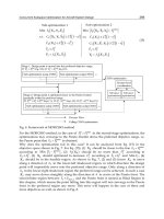
1. CHOOSE an initial random vector v

1
and NORMALIZE it.
2. FOR j=1,2, m DO:
(a) Calculate
w
j
as Cv
j
= w
j
. Which is equivalent to solve the problem Aw
j
= Bv
j
(A
non-symmetric).
(b) FOR i=1,2, j DO:
h
ij
=(Cv
j
, v
i
), (89)
a
=
j
∑
i=1
h

ij
v
i
, (90)
ˆ
v
j+1
= w
j
− a, (91)
h
j+1,j
= 
ˆ
v
j+1
, (92)
v
j+1
=
ˆ
v
j+1
h
j+1,j
(93)
END DO
END DO
This algorithm delivers an orthonormal basis V
m

=[v
1
, v
2
, , v
m
] of the Krylov subspace
K
m
= span{v
1
, Cv
1
, , C
m−1
v
1
}. The restriction from C to K
m
is represented by the matrix
H
m
= {h
ij
}. The eigenvalues of the latter matrix are an approximation of the m largest
eigenvalues of the original problem (65). The eigenvectors associated with these eigenvalues
may be obtained from
ˆ
q
i

= V
m
˜
y
i
(94)
where
˜
y
i
is an eigenvector of H
m
associated with the μ
i
-th eigenvalue.
Note that, since the matrix C is unknown a-priori, a non-symmetric linear system Cv
j
=
A
−1
Bv
j
= q
j
or, equivalently, Aq
j
= Bv
j
must be solved at each iteration, q
j

being an unknown
auxiliary vector. It is important to remark that the invert process needs the inversion of the A
operator which means that at least one LU or Incomplete-LU decomposition must be done.
The total time needed for a complete Arnoldi analysis depends mostly on the efficiency
of the linear solver described above, as well as on the Krylov space dimension m used to
approximate the most important eigenvalues.
In order to find the leading eigenvalue with maximum real part, one can use the shift and
invert strategy. If ω
0
is an approximation to the complex eigenvalue of interest, the shifted
and inverted problem is
(C −ω
0
)
−1
ˆ
q
= μ
ˆ
q (95)
where μ
= −(ω −ω
0
)
−1
.
5. Results
5.1 Single–domain spectral collocation computations
Selected results, representative of the applications to which the tools discussed earlier have
been applied, are briefly exposed next; full discussion of the respective applications may

212
Aeronautics and Astronautics
High-Order Numerical Methods for BiGlobal Flow Instability Analysis and Control 29
be found in the references provided. Starting with the single–domain spectral collocation
method on a rectangular domain, which has been the main approach applied to the solution
of the BiGlobal EVP by several authors Lin & Malik (1996a;b); Tatsumi & Yoshimura (1990);
Theofilis et al. (2003), attention is focused on the global instability of laminar separation
bubbles (LSBs) in the incompressible regime Theofilis et al. (2000), and on attachment–line
instability in compressible flow Duc et al. (2006); Theofilis, Fedorov & Collis (2004).
In the context of LSB flows, two approaches have been followed for the construction of
the basic flows, firstly an analytical one, making use of the attached and the separated
Falkner–Skan branches, and secondly an inverse boundary–layer method, in which the
wall–shear is prescribed. In the context of the first methodology, the instability analysis was
performed for bubbles with different Reynolds numbers, but the same value of m
lim
= −0.025.
All the bubbles analyzed have a peak reversed-flow higher than 10% of the reference velocity,
chosen in order to ensure proximity to conditions of amplification of the global mode Theofilis
et al. (2000). The amplitude functions of the global modes discovered in our previous work
were centered on the bubble and extended for only a short distance downstream. Analogous
boundary conditions were imposed here but substantially higher resolutions were required
in order to converge results at (displacement–thickness–based) Reynolds number Re
= 50.
Concretely, the system (30-33) been solved for the determination of the (direct) linear global
perturbations and convergence of the results has been attained using
(N
x
, N
y
)=(120,40)

spectral collocation points and a constant Krylov subspace dimension of 200. At these
parameters the discretized eigenvalue problem for each pair of the parameters (Re,β) required
the storage and inversion of a matrix with leading dimension 1.98
×10
4
, which translates on
6 Gbytes of memory. Though hardware was available in order to perform this work serially
in a shared–memory manner, all computations shown were performed in parallel.
The spanwise wavenumber parameter range 0
≈ β ≤ 35 has been examined and two global
modes have been identified. The first one is known from previous work Theofilis et al. (2000),
is steady (ω
r
= 0) and its periodicity length in the spanwise direction is approximately the
same of the bubble; at relatively high β values this mode is transformed into two travelling
modes (ω
r
= 0). The newly discovered mode is always a traveling instability with spanwise
periodicity length about a third of that of the bubble Rodríguez (2008). Both modes have been
encountered for Reynolds numbers, based on the displacement-thickness at inflow, below 100.
On the other hand, the solution of the adjoint BiGlobal EVP provides the spatial regions where
the receptivity of the basic flow to small perturbations is higher: the adjoint eigensolution field
defines the efficiency by which a particular forcing excites the direct eigensolution Hill (1992).
The adjoint BiGlobal EVP (39-42) has been solved next; the boundary conditions applied
to the direct problem are inverted here, as discussed in section 2. Dirichlet homogeneous
boundary conditions are imposed at the right-hand boundary while linear extrapolation from
the interior of the domain is imposed at the left. The amplitude functions recovered are again
centered in the bubble, but this time they are extend upstream. Some perturbation velocity
components seem to vanish at the left boundary of the domain.
Performing the same analysis for Re

δ
∗
= 500 at inflow, the eigenspectrum is symmetric,
and some branches can be identified corresponding to the global modes. The least stable
eigenmode founded here is the same steady mode present at lower Reynolds numbers, and
is depicted on figure 2 for the direct and adjoint eigenmodes . Much like the lower–Reynolds
number case, the spatial structure of the global modes is centered on the bubble, and extends
downstream for the direct eigenfunction and upstream for the adjoint Rodríguez & Theofilis
213
High-Order Numerical Methods for BiGlobal Flow Instability Analysis and Control