Aeronautics and Astronautics Part 7 pptx

High-Order Numerical Methods for BiGlobal Flow Instability Analysis and Control 45
Fig. 10. Upper: Amplitude functions of the least-damped eigenmode of geometry "in
1
"at
Re
= 1000, α = 1 González, Rodríguez & Theofilis (2008).Lower: Amplitude functions of the
least-damped eigenmode of geometry "in
2
"atRe = 1000, α = 1 González, Rodríguez &
Theofilis (2008). Left to right column:
ˆ
u
1
,
ˆ
u
2
,
ˆ
u
3
.
229
High-Order Numerical Methods for BiGlobal Flow Instability Analysis and Control
46 Will-be-set-by-IN-TECH
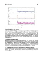
Fig. 11. Upper-Left: Leading eigenmode in the wake of the T106-300 LPT flow at Re = 890.
Upper-Right: Leading (wake) eigenmode in flow over an aspect ratio 8 ellipse at Re
= 200
Kitsios et al. (2008). Lower: Leading LPT Floquet mode at Re
= 2000 Abdessemed et al. (2004).
230

Aeronautics and Astronautics
High-Order Numerical Methods for BiGlobal Flow Instability Analysis and Control 47
6. Discussion
Numerical methods for the accurate and efficient solution of incompressible and compressible
BiGlobal eigenvalue problems on regular and complex geometries have been discussed. The
size of the respective problems warrants particular formulations for each problem intended to
be solved: the compressible BiGlobal EVP is only to be addressed when essential compressible
flow instability phenomena are expected, e.g. in the cases of shock–induced or supersonic
instabilities of hydrodynamic origin or in aeroacoustics research. In all other problems the
substantially more efficient incompressible formulation suffices for the analysis. Regarding
the issue of time–stepping versus matrix formation approaches, there exist distinct advantages
and disadvantages in either methodology; the present article highlights both, in the hope that
it will assist newcomers in the field to make educated choices. No strong views on the issue
of oder–of–accuracy of the methods utilized are offered, on the one hand because both low–
and high–order methods have been successfully employed to the solution of problems of this
class and on the other hand no systematic comparisons of the characteristics of the two types
of methods have been made to–date. Intentionally, no further conclusions are offered, other
than urging the interested reader to keep abreast with the rapidly expanding body of literature
on global linear instability analysis.
7. Acknowledgments
The material is based upon work sponsored by the Air Force Office of Scientific Research, Air
Force Material Command, USAF, under Grants monitored by Dr. J. D. Schmisseur of AFOSR
and Dr. Surya Surampudi of EOARD. The views and conclusions contained herein are those
of the author and should not be interpreted as necessarily representing the official policies or
endorsements, either expressed or implied, of the Air Force Office of Scientific Research or the
U.S. Government.
8. References
Abdessemed, N., Sherwin, S. J. & Theofilis, V. (2004). On unstable 2d basic states in low
pressure turbine flows at moderate reynolds numbers, number Paper 2004-2541 in
34th Fluid Dynamics Conference and Exhibit, AIAA, Portland, Oregon.

Abdessemed, N., Sherwin, S. J. & Theofilis, V. (2006). Linear stability of the flow past a low
pressure turbine blade, number Paper 2004-3530 in 36th Fluid Dynamics Conference
and Exhibit, AIAA, San Francisco, CA.
Abdessemed, N., Sherwin, S. J. & Theofilis, V. (2009). Linear instability analysis of low
pressure turbine flows, J. Fluid Mech. 628: 57 – 83.
Albensoeder, S., Kuhlmann, H. C. & Rath, H. J. (2001a). Multiplicity of steady
two-dimensional flows in two–sided lid–driven cavities, Theor. Comp. Fluid. Dyn.
14: 223–241.
Albensoeder, S., Kuhlmann, H. C. & Rath, H. J. (2001b). Three-dimensional centrifugal-flow
instabilities in the lid-driven-cavity problem, Phys. Fluids 13(1): 121–136.
Allievi, A. & Bermejo, R. (2000). A characteristic-finite element conjugate gradient algorithm
for the navier-sokes equations, Int. J. Numer. Meth. Fluids 32(*): 439–464.
Barkley, D. & Henderson, R. D. (1996). Three-dimensional floquet stability analysis of the
wake of a circular cylinder, J. Fluid Mech. 322: 215–241.
231
High-Order Numerical Methods for BiGlobal Flow Instability Analysis and Control
48 Will-be-set-by-IN-TECH
Bewley, T. R. (2001). Flow control: New challenges for a new renaissance, Progress in Aerospace
Sciences 37: 21–58.
Bres, G. & Colonius, T. (2008). Three-dimensional instabilities in compressible flow over open
cavities, J. Fluid Mech. 599: 309–339.
Broadhurst, M., Theofilis, V. & Sherwin, S. J. (2006). Spectral element stability analysis of
vortical flows, number Paper 2006-2877 in 6th IUTAM Laminar-Turbulent Transition
Symposium, Bangalore, India, Dec 13–17, 2004, pp. 153–158.
Collis, S. S., Joslin, R. D., Seifert, A. & Theofilis, V. (2004). Issues in active flow control: theory,
control, simulation and experiment, Prog. Aero. Sciences 40: 237–289.
Crouch, J. D., Garbaruk, A. & Magidov, D. (2007). Predicting the onset of flow unsteadiness
based on global instability, J. Comp. Phys. 224: 924–940.
Cuvelier, C., Segal, A. & van Steenhoven, A. A. (1986). Finite Element Methods and Navier-Stokes
Equations, D. Reidel Publishing Company.

de Vicente, J., Rodríguez, D., Theofilis, V. & Valero, E. (2011). Stability analysis in
spanwise-periodic double-sided lid-driven cavity flows with complex cross-sectional
profiles, Computers and Fluids 43: 143–153.
de Vicente, J., Valero, E., González, L. & V.Theofilis (2006). Spectral multi-domain methods
for biglobal instability analysis of complex flows over open cavity configurations,
number Paper 2006-2877 in 36th AIAA Fluid Dynamics Conference and Exhibit, AIAA,
San Francisco, California.
Ding, Y. & Kawahara, M. (1998). Linear stability of incompressible flow using a mixed finite
element method, J. Comp. Phys. 139: 243–273.
Dobrinsky, A. & Collis, S. S. (2000). Adjoint parabolized stability equations for receptivity
prediction, AIAA Paper 2000–2651.
Duc, A. L., Sesterhenn, J. & Friedrich, R. (2006). Instabilities in compressible attachment–line
boundary layers, Phys. Fluids 18: 044102–1–16.
Giannetti, F. & Luchini, P. (2007). Structural sensitivity of the first instability of the cylinder
wake, J. Fluid Mech. 581: 167 – 197.
González, L., Gómez-Blanco, R. & Theofilis, V. (2008). Eigenmodes of a counter-rotating vortex
dipole, AIAA J. DOI: 10.2514/1.35511: to appear.
González, L. M. & Bermejo, R. (2005). A semi-langrangian level set method for incompressible
navier-stokes equations with free surface, Int. J. Numer. Meth. Fluids 49(*): 1111–1146.
González, L., Rodríguez, D. & Theofilis, V. (2008). On instability analysis of realistic intake
flows, number Paper 2008-4380 in 38th Fluid Dynamics Conference and Exhibit, AIAA,
Seattle, WA.
González, L., Theofilis, V. & Gómez-Blanco, R. (2007). Finite element numerical methods for
viscous incompressible biglobal linear instability analysis on unstructured meshes,
AIAA J. 45: 840–855.
Gonzalez L, Theofilis V & Gomez-Blanco R (2007). Finite-element numerical methods for
viscous incompressible biglobal linear instability analysis on unstructured meshes,
AIAA Journal 45(4): 840–855.
Hein, S., Hohage, T., Koch, W. & Schoberl, J. (2007). Acoustic resonances in a high-lift
configuration, J. Fluid Mech. 582: 179–202.

Henningson, D. S. (1987). Stability of parallel inviscid schear flow with mean spanwise
variation, Tech. Rep. FFA-TN-1987-57, Bromma, Sweden.
Hill, D. C. (1992). A theoretical approach for the restabilization of wakes, AIAA Paper 92–0067.
232
Aeronautics and Astronautics
High-Order Numerical Methods for BiGlobal Flow Instability Analysis and Control 49
Karniadakis, G. E. & Sherwin, S. J. (2005). Spectral/hp element methods for CFD, OUP.
Kitsios, V., Rodríguez, D., Theofilis, V., Ooi, A. & Soria, J. (2008). Biglobal instability analysis
of turbulent flow over an airfoil at an angle of attack, number Paper 2008-4384 in 38th
Fluid Dynamics Conference and Exhibit, AIAA, San Francisco, CA.
Koch, W. (2007). Acoustic resonances in rectangular open cavities, AIAA J. 43: 2342–2349.
Leriche, E., Gavrilakis, S. & Deville, M. O. (1998). Direct simulation of the lid-driven
cavity flow with chebyshev polynomials, in K. D. Papailiou (ed.), Proc. 4th European
Computational Fluid Dynamics Conference, Vol. 1(1), ECCOMAS, pp. 220–225.
Lessen, M., Sadler, S. G. & Liu, T. Y. (1968). Stability of pipe poiseuille flow, Phys. Fluids
11: 1404–1409.
Lin, R S. & Malik, M. R. (1996a). On the stability of attachment-line boundary layers. Part 1.
the incompressible swept hiemenz flow, J. Fluid Mech. 311: 239–255.
Lin, R S. & Malik, M. R. (1996b). On the stability of attachment-line boundary layers. Part 2.
the effect of leading-edge curvature, J. Fluid Mech. 333: 125 – 137.
Mack, L. M. (1984). Boundary layer linear stability theory, AGARD–R–709 Special course on
stability and transition of laminar flow, pp. 3.1–3.81.
Malik, M. R. (1991). Numerical methods for hypersonic boundary layer stability, J. Comp. Phys.
86: 376–413.
Marquet, O., Sipp, D. & Jacquin, L. (2006). Global optimal perturbations in separated flow over
a backward-rounded -step, number Paper 2006-2879 in 3rd Flow Control Conference,
AIAA, San Francisco, CA.
Mayer, E. W. & Powell, K. G. (1992). Viscous and inviscid instabilities of a trailing vortex,
Journal of Fluid Mechanics 245: 91–114.
Morse, P. M. & Feshbach, H. (1953). Methods of Theoretical Physics, Parts I, II, McGraw-Hill.

Nayar, N. & Ortega, J. M. (1993). Computation of selected eigenvalues of generalized
eigenvalue problems, J. Comput. Physics 108: 8–14.
Poliashenko, M. & Aidun, C. K. (1995). A direct method for computation of simple
bifurcations, Journal of Computational Physics 121: 246–260.
Pralits, J. O. & Hanifi, A. (2003). Optimization of steady suction for disturbance control on
infinite swept wings, Phys. Fluids 15(9): 2756 – 2772.
Robinet, J C. (2007). Bifurcations in shock-wave/laminar-boundary-layer interaction: global
instability approach, J. Fluid Mech. 579: 85–112.
Rodríguez, D. (2008). On instability and active control of laminar separation bubbles,
Proceedings of the 4th PEGASUS-AIAA Student Conference, Prague .
Rodríguez, D. & Theofilis, V. (2008). On instability and structural sensitivity of incompressible
laminar separation bubbles in a flat–plate boundary layer, number Paper 2008-4148
in 38th AIAA Fluid Dynamics conference, Jan. 23-26, 2008, AIAA, Seattle, WA.
Rodríguez, D. & Theofilis, V. (2010). Structural changes of laminar separation bubbles induced
by global linear instability, J. Fluid Mech. p. (to appear).
Sahin, M. & Owens, R. G. (2003). A novel fully-implicit finite volume method applied to the
lid-driven cavity problem. part ii. linear stability analysis, Int. J. Numer. Meth. Fluids
42: 79–88.
Salwen, H., Cotton, F. W. & Grosch, C. E. (1980). Linear stability of poiseuille flow in a circular
pipe, J. Fluid Mech. 98: 273–284.
Schmid, P. J. & Henningson, D. S. (2001). Stability and transition in shear flows, Springer-Verlag,
New York.
233
High-Order Numerical Methods for BiGlobal Flow Instability Analysis and Control
50 Will-be-set-by-IN-TECH
Tatsumi, T. & Yoshimura, T. (1990). Stability of the laminar flow in a rectangular duct, J. Fluid
Mech. 212: 437–449.
Theofilis, V. (2000). Global linear instability in laminar separated boundary layer flow., in
H. Fasel & W. Saric (eds), Proc. of the IUTAM Laminar-Turbulent Symposium V, Sedona,
AZ, USA, pp. 663 – 668.

Theofilis, V. (2001). Inviscid gglobal linear instability of compressible flow on an elliptic
cone: algorithmic developments, Technical Report F61775-00-WE069, European Office
of Aerospace Research and Development.
Theofilis, V. (2003). Advances in global linear instability of nonparallel and three-dimensional
flows, Prog. Aero. Sciences 39 (4): 249–315.
Theofilis, V. (2009a). On multidimensional global eigenvalue problems for hydrodynamic and
aeroacoustic instabilities, number Paper 2009-0007 in 47th Aerospace Sciences Meeting
5–8 Jan. 2009, AIAA, Orlando, FL.
Theofilis, V. (2009b). The role of instability theory in flow control, in R. D. Joslin & D. Miller
(eds), Active Flow Control, AIAA Progress in Aeronautics and Astronautics Series,
AIAA.
Theofilis, V. (2011). Global linear instability, Annu. Rev. Fluid Mech. 43: 319–352.
Theofilis, V. (AIAA-2000-1965). Globally unstable basic flows in open cavities, 6th AIAA
Aeroacoustics Conference and Exhibit .
Theofilis, V., Barkley, D. & Sherwin, S. J. (2002). Spectral/hp element technology for flow
instability and control, Aero. J. 106(619-625).
Theofilis, V. & Colonius, T. (2003). An algorithm for the recovery of 2- and 3-d biglobal
instabilities of compressible flow over 2-d open cavities, AIAA Paper 2003-4143.
Theofilis, V. & Colonius, T. (2004). Three-dimensional instablities of compressible flow
over open cavities: direct solution of the biglobal eigenvalue problem, 34th Fluid
Dynamics Conference and Exhibit, AIAA Paper 2004-2544, Portland, Oregon.
Theofilis, V., Duck, P. W. & Owen, J. (2004). Viscous linear stability analysis of rectangular
duct and cavity flows, J. Fluid. Mech. 505: 249–286.
Theofilis, V., Fedorov, A. & Collis, S. S. (2004). Leading-edge boundary layer flow: PrandtlÂt’s
vision, current developments and future perspectives, IUTAM Symposium "One
Hundred Years of Boundary Layer Research", Göttingen, Germany, August 12-14, 2004,
Springer, pp. 73–82.
Theofilis, V., Fedorov, A., Obrist, D. & Dallmann, U. C. (2003). The extended
görtler-hämmerlin model for linear instability of three-dimensional incompressible
swept attachment-line boundary layer flow, J. Fluid Mech. 487: 271–313.

Theofilis, V., Hein, S. & Dallmann, U. C. (2000). On the origins of unsteadiness and
three-dimensionality in a laminar separation bubble, Phil. Trans. Roy. Soc. (London)
A 358: 3229–3246.
Trefethen, L. N. (2000). Spectral Methods in Matlab, SIAM.
Zhigulev, V. N. & Tumin, A. (1987). Origin of turbulence, Nauka .
234
Aeronautics and Astronautics
Part 2
Flight Performance, Propulsion, and Design

8
Rotorcraft Design for Maximized
Performance at Minimized Vibratory Loads
Marilena D. Pavel
Faculty of Aerospace Engineering, Delft University of Technology
The Netherlands
1. Introduction
Rotorcraft (helicopters and tiltrotors) are generally reliable flying machines capable of
fulfilling missions impossible with fixed-wing aircraft, most notably rescue operations.
These missions, however, often lead to high and sometimes excessive pilot workload.
Although high standards in terms of safety are imposed in helicopter design, studies show
that “it is ten times more likely to be involved in an accident in a helicopter than in a fixed-wing
aircraft” (Iseler et. al. 2001). According to World Aircraft Accident Summary (WAAS, 2002),
nearly 45 percent of all accidents of single-piston helicopters is attributed to pilot loss of
control, where - because of various causes, often involving vibrations, high workload, and
bad weather - a pilot loses control of the helicopter and crashes, sometimes with fatal
consequences. Quoting the Royal Netherlands Air Force (‘Veilig Vliegen’ magazine, 2003),
“for helicopters there is a considerable number of inexplicable incidents (…) which involved piloting
loss of control”. The situation is likely to get worse, as rotorcraft missions are becoming more
difficult, demanding high agility and rapid manoeuvring, and producing more violent

vibrations. (Kufeld & Bousman, 1995; Hansford & Vorwald, 1996; Datta & Chopra, 2002)
The primary cause of pilot control difficulties and high-workload situations is that even
modern helicopters often have poor Handling Qualities (HQs) (Padfield, 1998). Cooper and
Harper (Cooper & Harper, 1969), pioneers in this subject, defined these as: “those qualities or
characteristics of an aircraft that govern the ease and precision with which a pilot is able to perform a
mission”. Below, the current practice in rotorcraft handling qualities assessment will be
discussed, introducing the key problem addressed in this chapter.
1.1 State-of-the-art in rotorcraft handling qualities – The aeronautical design standard
ADS-33
Helicopter handling qualities used to be assessed with requirements defined for fixed-wing
aircraft, as stated in the FAR (civil) and MIL (military) standards. In the 1960’s, however, it
became clear that these standards were not sufficient (Key, 1982). Helicopters have strong
cross-coupling effects between longitudinal and directional controls, their behaviour is highly
non-linear and requires more degrees of freedom in modelling than the rigid-body models used
for aircraft. Therefore, the MIL-H-8501A standard (MIL-H-8501A, 1962) was developed. This
standard was used up until mid 1980’s. From a safety perspective, these requirements were
merely ‘good minimums’, and a new standard was developed in the 1970’s, that is used up
until today, the Aeronautical Design Standard ADS-33 (ADS-33, 2000)

Aeronautics and Astronautics

238
The crucial point, understood by ADS-33, is that helicopter HQ requirements need to be
related to the mission executed, as this will determine the needed pilot effort. E.g., a
shipboard landing at night and in high sea with strong ship motions demands more
precision of control from the pilot than when flying in daytime and good weather.2 ADS-
33 introduced handling qualities metrics (HQM), a combination of flight parameters such as
rate of climb, turn rate, etc., that reflect how much manoeuvre-capability the pilot has per
specific mission. These metrics are then mapped into handling qualities criteria (HQC) that
yield boundaries between ‘good’ (Level 1), ‘satisfactory’ (Level 2) and ‘poor’ (Level 3)

HQs.
1

Despite their importance for the helicopter safety, its operators and, above all, the
helicopter pilots, achieving good handling qualities is still mainly a secondary goal in
helicopter design. The first phase in helicopter design is the ‘conceptual design’ phase in
which the main rotor and fuselage parameters are established, based on desired
performance and, to some extent, vibration criteria.20 Only in the following phase, that of
preliminary design, are ‘high-fidelity’ simulation models developed and the handling
qualities considered. The high fidelity models allow an analysis of helicopter behaviour
for various flight conditions. Applying the ADS-33 metrics/criteria to these models
results in predicted levels of HQs. When these are known, the experimental HQ assessment
begins, illustrated in Fig. 1.

Missions
Defining OFE/SFE
Airspeed (kts)
Load
factor
1
2
3
0
50 100 150 2000
OFE
SFE
Control
loads
Blade
stall

Tail
stress
RPM droop
Gravity fed
hydraulics
A
D
S
-
3
3
Defining OFE/SFE
Airspeed (kts)
Load
factor
1
2
3
0
50 100 150 2000
OFE
SFE
Control
loads
Blade
stall
Tail
stress
RPM droop
Gravity fed

hydraulics
Defining OFE/SFE
Airspeed (kts)
Load
factor
1
2
3
0
50 100 150 2000
OFE
SFE
Control
loads
Blade
stall
Tail
stress
RPM droop
Gravity fed
hydraulics
Airspeed (kts)
Load
factor
1
2
3
0
50 100 150 2000
OFE

SFE
Control
loads
Blade
stall
Tail
stress
RPM droop
Gravity fed
hydraulics
A
D
S
-
3
3
Example of mission in the
simulator of Univ. of Liverpool
Missions
Defining OFE/SFE
Airspeed (kts)
Load
factor
1
2
3
0
50 100 150 2000
OFE
SFE

Control
loads
Blade
stall
Tail
stress
RPM droop
Gravity fed
hydraulics
Defining OFE/SFE
Airspeed (kts)
Load
factor
1
2
3
0
50 100 150 2000
OFE
SFE
Control
loads
Blade
stall
Tail
stress
RPM droop
Gravity fed
hydraulics
Airspeed (kts)

Load
factor
1
2
3
0
50 100 150 2000
OFE
SFE
Control
loads
Blade
stall
Tail
stress
RPM droop
Gravity fed
hydraulics
A
D
S
-
3
3
Defining OFE/SFE
Airspeed (kts)
Load
factor
1
2

3
0
50 100 150 2000
OFE
SFE
Control
loads
Blade
stall
Tail
stress
RPM droop
Gravity fed
hydraulics
Airspeed (kts)
Load
factor
1
2
3
0
50 100 150 2000
OFE
SFE
Control
loads
Blade
stall
Tail
stress

RPM droop
Gravity fed
hydraulics
Defining OFE/SFE
Airspeed (kts)
Load
factor
1
2
3
0
50 100 150 2000
OFE
SFE
Control
loads
Blade
stall
Tail
stress
RPM droop
Gravity fed
hydraulics
Airspeed (kts)
Load
factor
1
2
3
0

50 100 150 2000
OFE
SFE
Control
loads
Blade
stall
Tail
stress
RPM droop
Gravity fed
hydraulics
A
D
S
-
3
3
Airspeed (kts)
Load
factor
1
2
3
0
50 100 150 2000
OFE
SFE
Control
loads

Blade
stall
Tail
stress
RPM droop
Gravity fed
hydraulics
Airspeed (kts)
Load
factor
1
2
3
0
50 100 150 2000
OFE
SFE
Control
loads
Blade
stall
Tail
stress
RPM droop
Gravity fed
hydraulics
A
D
S
-

3
3
Example of mission in the
simulator of Univ. of Liverpool

Fig. 1. Experimental assessment of helicopter handling qualities

1
Level 1 HQs means that the rotorcraft is satisfactory without improvements required from the pilot’s
perspective. Level 2 HQs means that pilots can achieve adequate performance, but with compensation;
at the extreme of Level 2, the mission is flyable, but pilots have little capacity for other duties and can
not sustain flying for longer periods without the danger of pilot error. Level 3 HQs is unacceptable, it
describes rotorcraft behaviour in extreme situations, like the loss of critical flight control systems.

Rotorcraft Design for Maximized Performance at Minimized Vibratory Loads

239
In this process, first databases of missions and environments are defined, according to
customer requirements. Manoeuvrability, i.e., how easy can pilots guide the helicopter,
and agility, i.e., how quickly can they change its flight direction, are critical performance
demands. Second, experienced test pilots are asked to fly the missions in a flight
simulator. Through insisting pilots to execute the mission very thoroughly, one aims to
expose deficient handling qualities. Pilots rate the HQs they experience in each
manoeuvre flown, generally using the Cooper-Harper rating scale.
2
Third, Operational
Flight Envelopes (OFEs) and Service Flight Envelopes (SFEs) are defined, based on a
mapping of the HQ ratings. OFEs represent the limits within which the helicopter must be
able to operate in order to accomplish the operational missions. SFEs stem from the
helicopter limits and are expressed in terms of any parameters believed necessary to

ensure safety, see Fig. 1.
In this first experimental assessment of the helicopter’s handling qualities, the first problems
arise, as more often than not, large differences arise between the theoretical predictions and
the experimentally-determined pilot judgments. The gaps that occur are bridged by
applying optimisation techniques using the simulation models developed in preliminary
design, to improve the designs of helicopter, load alleviation system and flight control
system (Celi, 1991; Celi, 1999; Celi, 2000; Fusato & Celi, 2001, Fusato & Celi, 2002a,2002b;
Ganduli, 2004; Sahasrabudhe & Celi, 1997). Computational approaches have three important
disadvantages, however. First, many designs that “roll out” of the procedure are unfeasible,
the optimisation “pushing” the solution along the boundaries of the problem and not inside
of the feasible region. Second, optimising for ADS-33 requires calculations of the helicopter
time-domain responses, and the numerical methods become computationally very intensive
(Sahasrabudhe & Celi, 1997; Tischler et. al., 1997) Third, and most important, the lack of
quantitative, validated helicopter pilot models, capable of accurately predicting the effects of
helicopter vibrations on pilot control behaviour, prevents the proper inclusion of pilot-
centred considerations in mathematical optimization techniques (Mitchell et. al., 2004;
Tischler et. al., 1996)
Whereas the first and second disadvantages are common in multi-dimensional design
problems, the lack of knowledge on how helicopter vibrations affect pilot performance is a
typical and fundamental problem of modern helicopter design (Mitchell et. al., 2004,
Padfield, 1998). Although ADS-33 proposes criteria and missions regarding helicopter
limits, these only characterize a helicopter’s performance, and do not require an adequate
knowledge of helicopter vibratory loads (Kolwey, 1996; Tischler et. al., 1996). This
shortcoming stems from the fact that, when the ADS-33 criteria were defined, helicopter
missions were not so demanding, and the vibratory loads associated with them were low. In
the last twenty years, however, ever-increasing performance requirements and extended
flight envelopes were defined, for reasons of heavy competition, demanding manoeuvres
that impose heavy vibrations on both structure and pilot. These vibrations, combined with
cross-coupling effects, rapidly lead to pilot overload and degradation in performance
(Padfield, 2007).

Key Problem: The current practice of assessing rotorcraft handling qualities reveals
significant gaps in the ADS-33 HQ criteria, especially regarding the effects of vibrations.

2
The Cooper-Harper rating scale runs from 1 to 10. Rates from 1 to 3 1/2 correspond to Level 1 HQs; rates
from 31/2 to 61/2 correspond to Level 2 HQs, and rates from 61/2 up to 10 correspond to Level 3 HQs.


Aeronautics and Astronautics

240
1.2 Goal
The design of high-performance rotorcraft has become an arduous process, regularly
leading to surprises, demanding ‘patches’ to safety-critical systems, and needing more
iterations than expected, all contributing in very high costs. Unmistakably, the helicopter
and flight control system design teams do not have up-to-date criteria to adequately assess
the effects of helicopter vibrations on its handling qualities. There is an urgent need for a
much more fundamental understanding of how helicopter vibrations affect pilot control
behaviour (Mitchell et. al., 2004) and for new tools to incorporate this knowledge as early as
possible in the design of both helicopter and flight control system. The goal of this chapter is
to portray a novel approach to rotorcraft handling qualities (HQs) assessment by defining a
set of consistent, complementary metrics for agility and structural loads pertaining to
vertical manoeuvres in forward flight. These metrics can be used by the designer for making
trade—offs between agility and vibrational/load suppression. The emphasis of the chapter
will be on agility characteristics in the pitch axis applied to helicopter and tiltrotor.
Especially in such new configurations, the proposed approach could be particularly useful
as the performance tools for fixed-wing mode and helicopter mode must merge together
within new criteria (Padfield, 2008).
The chapter is structured as follows: The second section will present an overview of
traditional metrics for measuring pitch agility; The third section will present some

alternative metrics proposed in the 90’s for better capturing the transient characteristics of
the agility; Then, based on the rational developments of the metrics from the previous two
sections, fourth section will propose the new approach that can better quantify the agility
from the designer point of view. Finally, general conclusions and potential extension of this
work will be discussed.
2. Traditionally design of aircraft for pitch agility
One of the most important flying quality concepts defining the upper limits of performance
is the so-called “agility”. Generally, it is well known that the level of performance achieved
by the pilot depends on the task complexity. Fig. 2 presents generically this situation,
showing that there is a line of saturation up to which the pilot is able to perform optimally
the specified mission; increasing the task difficulty above this line leads quickly to stress,
panic and even incapacity to cope anymore with the task complexity and blocking,
sometimes with fatal consequences.
It is difficult to point precisely to the origins of the concept of agility but probably these
go back to the moment when it was realized that, in a combat, a “medium performance”
fighter could win over its superior opponent if the first aircraft possesses the potential for
faster transient motions, i.e. superior agility. In its most general sense, the concept of
agility is defined with respect to the overall combat effectiveness in the so-called
“Operational agility”. Operational agility according to measures the ‘ability to adapt and
respond rapidly and precisely, with safety and poise, to maximize mission effectiveness’(McKay,
1994). In the mid 80’s a strong wave of interest arose in seeking metrics and criteria that
could quantify the aircraft agility (Mazza, 1990; McKay, 1994). However, there have been
developed almost as many criteria of agility as there were investigators in the field. The
problem was partially due to the lack of coordination in the research studies performed
but also due to a disagreement on the most fundamental level: there simply was very little
agreement on what agility was.

Rotorcraft Design for Maximized Performance at Minimized Vibratory Loads

241

P
e
r
f
o
r
m
a
n
c
e
Optimum
Stress
Panic
Block
Level
performance
High
Low
High
Low
Level task difficulty
Relation between
TASK DIFFICULTY AND PERFORMANCE
P
e
r
f
o
r

m
a
n
c
e
Optimum
Stress
Panic
Block
Level
performance
High
Low
High
Low
Level task difficulty
Relation between
TASK DIFFICULTY AND PERFORMANCE

Fig. 2. Correlation between task difficulty and performance
Within the framework of operational agility one can see agility as a function of the airframe,
avionics, weapons and pilot. Airframe agility is probably the most crucial component in the
operational agility as it is designed in from the onset and cannot be added later. The present
chapter focuses on airframe agility and within this, the chapter will relate to the airframe
agility in the pitch axis.
A large number of agility metrics have been proposed during the years to determine the
aircraft realm of agility. The AGARD Working Group 19 on Operational Agility (McKay,
1994) put together all the different metrics and criteria existing on agility and fit them into a
generalizable framework for further agility evaluations. The present section presents the
traditional approach on pitch agility using as example a tiltrotor aircraft. This specific

aircraft combines the properties of both fixed and rotary-wing aircraft and can be used to
define a unified approach in the agility requirements at both fixed and rotary-wings.
The tiltrotor example to be investigated in this study is the Bel XV-15 aircraft. Next, as
vehicle model, the FLIGHTLAB model of the Bell XV-15 aircraft as developed by the
University of Liverpool (this model is designated as FXV-15) will be used. For a complete
description of this model and the assumptions made the reader is referred to (Manimala et.
al., 2003). For the tiltrotor in helicopter mode, the pilot’s controls command pitch through
longitudinal cyclic, roll through differential collective (lateral cyclic is also provided for
trimming), yaw through differential longitudinal cyclic and heave through combined
collective. In airplane mode, the pilot controls command conventional elevator, aileron and
rudder (a small proportion of differential collective is also included).
Pitch agility is the ability to move, rapidly and precisely, the aircraft nose in the longitudinal
plane and complete with easiness that movement. This implies that in the agility analysis
one has to search for sample manoeuvres to be carried out by the flight vehicle dominated
by high flight path changes and high rate of change of longitudinal acceleration which can
give a good picture of the agility characteristics. As starting point in this discussion on pitch

Aeronautics and Astronautics

242
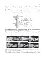
agility we will consider the kinematics of a sharp pitch manoeuvre – a simple example of
this type is the tiltrotor trying to fly over an obstacle (see Fig. 3). Assume that the
manoeuvre is executing starting from different forward speeds (helicopter mode 60 kts and
120kts; airplane mode 120 kts and 300 kts) and the manoeuvre aggressiveness is varied by
varying the pulse duration (from 1 to 5 sec). The pilot flies the manoeuvre by giving a pulse
input in the longitudinal cyclic stick of 1 inch amplitude.


Fig. 3. Executing an obstacle-avoid manoeuvre in the pitch axis
2.1 Transient metrics

The first class of metrics developed to quantify the agility corresponds to the so-called
“transient metrics”. The transient class contains metrics which can be calculated at any
moment for any manoeuvre. For pitch agility these metrics are pitch rate (entitled attitude
manoeuvrability metric) and accelerations along the axes a
x
, a
y
, a
z
(entitled manoeuvrability
of the flight path). These metrics are next studied for the pull up manoeuvres flown with the
FXV-15 in a 1 second pulse given from the initial trim at 120kts in helicopter mode and 300
kts in airplane mode. The presentation of the transient metric information is best achieved
through a time history plot. Fig. 4 presents the transient metrics parameters of pitch rate q
and vertical acceleration n
z
(in the form of normal load factor). Looking at Fig. 4 one may see
local maxima in the metric parameters q and n
z
illustrating peak events in the agility
characteristics. This clearly demonstrates that in a “real” manoeuvre sequence, the agility
characteristics occur at key moments, depending on the manoeuvre.
2.2 Experimental metrics
The above conclusion gave the idea to develop a new class of agility metrics, the so-called
“experimental metrics” formulated as discrete parameters during a real manoeuvre
sequence. These metrics are actually the basic building blocks for understanding the agility
and can be related to flying qualities and aircraft design. The metrics describing pitch agility
during aggressive manoeuvring in vertical plane were defined by (Murphy et. al., 1991) and
are described in the next section. They referred to the ability of an aircraft to pint the nose in
at an opponent and commented that what was not clear in such manoeuvres was the

behaviour of the flight path. Was the nose pointing w.r.t. the velocity vector or did it include
the flight path bending or perhaps both? The authors noted that longitudinal stick
displacements would be expected to command the flight path in addition to the aircraft nose
pointing pitch angle for agile aircraft. The study pointed out that current aircraft behave
differently in the high speeds and slow speed regimes. In the high speed case the flight path
displaced as per the nose pointing displacement. The low speed case exhibited no flight path
or even opposite flight path displacements.

Rotorcraft Design for Maximized Performance at Minimized Vibratory Loads

243
0 1 2 3 4 5 6
0
0.5
1
0 1 2 3 4 5 6
-5
0
5
0 1 2 3 4 5 6
1
1.1
1.2
Longitudinal
cyclic stick
(in)
Pitch rate q
(deg/sec)
Load Factor
n

z
Forward flight V=120 kts 1 sec pulse
Helicopter mode
Pitch rate q
(deg/sec)
Load Factor
n
z
0 1 2 3 4 5 6
-10
0
10
0 1 2 3 4 5 6
1
1.5
2
2.5
time (sec)
Forward flight V=300 kts 1 sec pulse
Airplane mode
time (sec)
0 1 2 3 4 5 6
0
0.5
1
0 1 2 3 4 5 6
-5
0
5
0 1 2 3 4 5 6

1
1.1
1.2
0 1 2 3 4 5 6
0
0.5
1
0 1 2 3 4 5 6
-5
0
5
0 1 2 3 4 5 6
1
1.1
1.2
Longitudinal
cyclic stick
(in)
Pitch rate q
(deg/sec)
Load Factor
n
z
Forward flight V=120 kts 1 sec pulse
Helicopter mode
Pitch rate q
(deg/sec)
Load Factor
n
z

0 1 2 3 4 5 6
-10
0
10
0 1 2 3 4 5 6
1
1.5
2
2.5
time (sec)
0 1 2 3 4 5 6
-10
0
10
0 1 2 3 4 5 6
1
1.5
2
2.5
time (sec)
Forward flight V=300 kts 1 sec pulse
Airplane mode
time (sec)

Fig. 4. Transient agility metrics for pull-up manoeuvres with the tiltrotor
2.2.1 Peak and time to peak pitch rates
The peak and time to peak pitch rates metrics were proposed by (Murphy et. al., 1991) for
fixed wing aircraft. These metrics measure the time to reach peak pitch rate and the
corresponding pitch rate. Fig. 5 presents charts of peak pitch rate and time to reach this peak
as a function of the velocity for the tiltrotor flying pull-up manoeuvres of increasing pulse

duration. The pull-up manoeuvres are executed gradually increasing the velocity and the
nacelle angle from the helicopter mode (90deg nacelle, hover and 60 kts) to conversion
(60deg nacelle 120 kts) and ending in airplane mode (0deg nacelle 200 kts). Looking at these
figures one can see that as the velocity increases the pilot is able to achieve higher pitch
rates, the time to achieve these peaks being and faster especially if the pulse duration is
short. As attributes, the peak and time to peak pitch rates metrics have the advantage that
can be related to design.

Aeronautics and Astronautics

244
Peak pitch rates
in pull-up manoeuvres
0 20 40 60 80 100 120 140 160 180 200
0
10
20
30
40
50
60
70
1
i
n

i
n
p
u

t

1

s
e
c
1
i
n

i
n
p
u
t

5

s
e
c
v
H90
o
H90
o
C60
o
A0

o
1
i
n

i
n
p
u
t

2

s
e
c
H90
o
H90
o
H90
o
H90
o
C60
o
C60
o
A0
o

A0
o
q
pk
(deg/sec)
Velocity (kts)
H90
o
= 90
o
nacelle, helicopter mode
C60
o
= 60
o
nacelle, conversion mode
A0
o
= 0
o
nacelle, airplane mode
I
n
c
r
e
a
s
i
n

g

p
u
l
s
e

d
u
r
a
t
i
o
n
Peak pitch rates
in pull-up manoeuvres
0 20 40 60 80 100 120 140 160 180 200
0
10
20
30
40
50
60
70
1
i
n

i
n
p
u
t

1

s
e
c
1
i
n

i
n
p
u
t

5

s
e
c
v
H90
o

H90
o
C60
o
A0
o
1
i
n

i
n
p
u
t

2

s
e
c
H90
o
H90
o
H90
o
H90
o
C60

o
C60
o
A0
o
A0
o
q
pk
(deg/sec)
Velocity (kts)
H90
o
= 90
o
nacelle, helicopter mode
C60
o
= 60
o
nacelle, conversion mode
A0
o
= 0
o
nacelle, airplane mode
I
n
c
r

e
a
s
i
n
g

p
u
l
s
e

d
u
r
a
t
i
o
n
0 20 40 60 80 100 120 140 160 180 200
0
0.5
1
1.5
2
2.5
3
1

i
n
i
np
ut

1

s
e
c
1
i
n

i
n
p
u
t

2

s
e
c
1
i
n

i
n
p
u
t

3

s
e
c
1
i
n

i
n
p
u
t
4

s
e
c
H90
o
H90
o
H90

o
H90
o
H90
o
H90
o
H90
o
C60
o
C60
o
C60
o
C60
o
A0
o
A0
o
Time to Peak pitch rate
in pull-up manoeuvres
(sec)
pk
q
t |
Velocity (kts)
fast
slow

0 20 40 60 80 100 120 140 160 180 200
0
0.5
1
1.5
2
2.5
3
1
i
n
i
np
ut

1

s
e
c
1
i
n

i
n
p
u
t

2

s
e
c
1
i
n

i
n
p
u
t

3

s
e
c
1
i
n

i
n
p
u
t
4

s
e
c
H90
o
H90
o
H90
o
H90
o
H90
o
H90
o
H90
o
C60
o
C60
o
C60
o
C60
o
A0
o
A0
o

Time to Peak pitch rate
in pull-up manoeuvres
(sec)
pk
q
t |
Velocity (kts)
fast
slow

Fig. 5. Peak and time to peak pitch rates in pull-up manoeuvres
2.2.2 Peak and time to peak pitch accelerations
(Murphy et. al., 1991) considered the so-called peak and timer to peak pitch accelerations as
the primary metrics for pitch motion agility. The time to peak acceleration provides insight
into the jerk characteristics of pitch motion: if it is too slow, then the pilot may complain that
the aircraft is too sluggish for tracking-type tasks; if it is too fast, then the pilot may
complain of jerkiness or over-sensitivity. Fig. 6 presents charts of peak and time to leak pitch
acceleration as a function of velocity when flying pull-ups manoeuvres. One can see that as
the velocity increases the pilot is able to obtain higher pitch accelerations but as is passing
from the helicopter to aircraft mode this capability diminishes. For fixed wing aircraft,
(Murphy et. al., 1991) commented on the differences in the data for the peak accelerations in
the body and wind axes. This effect has implications on the pilot selection of flight path or
nose pointing control during manoeuvring.

Rotorcraft Design for Maximized Performance at Minimized Vibratory Loads

245


0 20 40 60 80 100 120 140 160 180 200

15
20
25
30
35
40
45
50
55
60
Peak pitch angle acceleration
in pull-up manoeuvres
(deg/sec
2
)
pk
q

Velocity (kts)
H90
o
H90
o
C60
o
A0
o
H90
o
= 90

o
nacelle, helicopter mode
C60
o
= 60
o
nacelle, conversion mode
A0
o
= 0
o
nacelle, airplane mode
H90
o
H90
o
H90
o
C60
o
C60
o
A0
o
1i
n

i
n
p

u
t

1
sec
I
n
c
r
e
a
s
i
n
g

p
u
l
s
e
d
u
r
a
t
i
o
n
1

i
n

i
n
p
u
t

3

s
e
c
1
i
n

i
n
p
u
t

5

s
e
c
0 20 40 60 80 100 120 140 160 180 200

15
20
25
30
35
40
45
50
55
60
Peak pitch angle acceleration
in pull-up manoeuvres
(deg/sec
2
)
pk
q

Velocity (kts)
H90
o
H90
o
C60
o
A0
o
H90
o
= 90

o
nacelle, helicopter mode
C60
o
= 60
o
nacelle, conversion mode
A0
o
= 0
o
nacelle, airplane mode
H90
o
H90
o
H90
o
C60
o
C60
o
A0
o
1i
n

i
n
p

u
t

1
sec
I
n
c
r
e
a
s
i
n
g

p
u
l
s
e
d
u
r
a
t
i
o
n
1

i
n

i
n
p
u
t

3

s
e
c
1
i
n

i
n
p
u
t

5

s
e
c

0 20 40 60 80 100 120 140 160 180 200
0
0.005
0.01
0.015
0.02
0.025
0.03
0.035
0.04
Time to peak pitch angle acceleration
in pull-up manoeuvres
pk
q
t

|
H90
o
H90
o
C60
o
A0
o
H90
o
H90
o

H90
o
H90
o
C60
o
A0
o
1
i
n

i
n
p
u
t

1

s
e
c
1
i
n

i
n
p

u
t

3

s
e
c
1
i
n

i
n
p
u
t

5

s
e
c
Velocity (kts)
I
n
c
r
e
a

s
i
n
g

p
u
l
s
e

d
u
r
a
t
i
o
n
fast
(sec)
0 20 40 60 80 100 120 140 160 180 200
0
0.005
0.01
0.015
0.02
0.025
0.03
0.035

0.04
Time to peak pitch angle acceleration
in pull-up manoeuvres
pk
q
t

|
H90
o
H90
o
C60
o
A0
o
H90
o
H90
o
H90
o
H90
o
C60
o
A0
o
1
i

n

i
n
p
u
t

1

s
e
c
1
i
n

i
n
p
u
t

3

s
e
c
1
i

n

i
n
p
u
t

5

s
e
c
Velocity (kts)
I
n
c
r
e
a
s
i
n
g

p
u
l
s
e

d
u
r
a
t
i
o
n
fast
(sec)

Fig. 6. Peak and time to peak pitch angle acceleration in pull-ups with the tiltrotor
2.2.3 Peak and time to peak load factor
Peak and time to peak load factor metrics describe the peak and the transition time to the
peak normal load factor during a manoeuvre in pitch axis. They can be used at best to
determine the flight path bending capability of an aircraft. Fig. 7 presents these two
metrics as a function of the velocity for the tiltrotor example. One may see that as the
velocity increases the pilot is able to pull more g’s as going from the airplane to helicopter
mode.

Aeronautics and Astronautics

246
0 20 40 60 80 100 120 140 160 180 200
1
1.1
1.2
1.3
1.4

1.5
1.6
1.7
1.8
1.9
2
1
i
n

i
n
p
u
t

1

s
e
c
1
i
n

i
n
p
u
t

3

s
e
c
1
i
n

i
n
p
u
t

5

s
e
c
H90
o
H90
o
H90
o
H90
o
C60

o
C60
o
C60
o
A0
o
A0
o
A0
o
Peak normal factor
in pull-up manoeuvres
n
z pk
(g’s)
Velocity (kts)
H90
o
= 90
o
nacelle, helicopter mode
C60
o
= 60
o
nacelle, conversion mode
A0
o
= 0

o
nacelle, airplane mode
0 20 40 60 80 100 120 140 160 180 200
1
1.1
1.2
1.3
1.4
1.5
1.6
1.7
1.8
1.9
2
1
i
n

i
n
p
u
t

1

s
e
c
1

i
n

i
n
p
u
t

3

s
e
c
1
i
n

i
n
p
u
t

5

s
e
c
H90

o
H90
o
H90
o
H90
o
C60
o
C60
o
C60
o
A0
o
A0
o
A0
o
Peak normal factor
in pull-up manoeuvres
n
z pk
(g’s)
Velocity (kts)
H90
o
= 90
o
nacelle, helicopter mode

C60
o
= 60
o
nacelle, conversion mode
A0
o
= 0
o
nacelle, airplane mode
Time to Peak normal load factor
in pull-up manoeuvres
0 50 100 150 200 250 300
0
0.5
1
1.5
2
2.5
3
3.5
4
4.5
5
H90
o
H90
o
C60
o

A0
o
A0
o
A0
o
A0
o
C60
o
A0
o
A0
o
C60
o
H90
o
H90
o
H90
o
Velocity (kts)
pkz
n
t |
(sec)
Time to Peak normal load factor
in pull-up manoeuvres
0 50 100 150 200 250 300

0
0.5
1
1.5
2
2.5
3
3.5
4
4.5
5
H90
o
H90
o
C60
o
A0
o
A0
o
A0
o
A0
o
C60
o
A0
o
A0

o
C60
o
H90
o
H90
o
H90
o
Velocity (kts)
pkz
n
t |
(sec)

Fig. 7. Peak and time to peak normal load factor
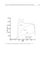
2.2.4 Pitch attitude quickness parameter
One of the most important pitch agility metrics introduced by ADS-33 helicopter standard
(ADS-33, 2000) is the so-called “pitch attitude quickness” parameter and is defined as the
ratio of the peak pitch rate to the pitch angle change:


1
sec
def
pk
q
Q






(1)
The advantage of this parameter is that it was linked to handling qualities so that potential
bounds for agility could be identified. In this sense, ADS-33 presents HQs boundaries for the
pitch quickness parameter as a function of the minimum pitch angular change 
min


Rotorcraft Design for Maximized Performance at Minimized Vibratory Loads

247
(considered as the pitch angle corresponding to a 10% decay from q
pk
). These boundaries are
defined to separate different quality levels, but because they relate too to an agility metric, they
become now boundaries of available agility. Fig. 8 illustrates the attitude quickness charts for
the tiltrotor executing pull-up maneuvers of 1 to 5 sec 1in amplitude input at 60, 120 and 300
kts in helicopter and airplane mode. The figure shows also the Level 1/2 boundaries as
defined by 1) ADS-33 for a general mission task element, low speed helicopter flight (<45kts)
and 2) MIL STD 1797A for fixed wing aircraft. One may see that whereas in helicopter mode
FXV-15 hardly meets Level 1 performance in ADS-33 standard, being mostly at Level 2
performance, in airplane mode FXV-15 meets Level 1 performance in AHS-33 but exhibits
Level 2 performance according to the MIL standard for airplanes (MIL HDBK-1797, 1997).

0 5 10 15 20 25 30
0
0.5
1

1.5
2
2.5
1 sec
2 sec
3 sec
4 sec
5 sec
1 sec
1 sec
1 sec
2 sec
3 sec
4 sec
5 sec
5 sec
5 sec
3 sec
M
I
L

S
T
D

1
7
9
7

A

L
e
v
e
l

1
/
2

b
o
u
n
d
a
r
y
A
D
S
-
3
3
E

L
e

v
e
l

1
/
2

b
o
u
n
d
a
r
y
60kts,1in helicopter mode
120kts, 1in helicopter mode
120kts, 1in airplane mode
300kts, 1in airplane mode
Level 1 MIL
Level 2 MIL
Level 1 ADS
Level 2 ADS

sec/1


pk
q

(deg)
min


0 5 10 15 20 25 30
0
0.5
1
1.5
2
2.5
1 sec
2 sec
3 sec
4 sec
5 sec
1 sec
1 sec
1 sec
2 sec
3 sec
4 sec
5 sec
5 sec
5 sec
3 sec
M
I
L

S
T
D

1
7
9
7
A

L
e
v
e
l

1
/
2

b
o
u
n
d
a
r
y
A
D

S
-
3
3
E

L
e
v
e
l

1
/
2

b
o
u
n
d
a
r
y
60kts,1in helicopter mode
120kts, 1in helicopter mode
120kts, 1in airplane mode
300kts, 1in airplane mode
Level 1 MIL
Level 2 MIL

Level 1 ADS
Level 2 ADS
0 5 10 15 20 25 30
0
0.5
1
1.5
2
2.5
1 sec
2 sec
3 sec
4 sec
5 sec
1 sec
1 sec
1 sec
2 sec
3 sec
4 sec
5 sec
5 sec
5 sec
3 sec
M
I
L

S
T

D

1
7
9
7
A

L
e
v
e
l

1
/
2

b
o
u
n
d
a
r
y
A
D
S
-

3
3
E

L
e
v
e
l

1
/
2

b
o
u
n
d
a
r
y
60kts,1in helicopter mode
120kts, 1in helicopter mode
120kts, 1in airplane mode
300kts, 1in airplane mode
Level 1 MIL
Level 2 MIL
Level 1 ADS
Level 2 ADS


sec/1


pk
q
(deg)
min



Fig. 8. Pitch quickness for the tiltrotor
3. Flying qualities metrics for agility designing
Linking the agility to flying qualities raised up a new question: is agility limited by pilot
handling parameters or in other words what are the upper limits to agility set by flying
qualities considerations? Flying qualities considerations do limit agility according to
(Padfield, 1998). In this sense, in a series of flight and simulation trials research conducted at
DERA (now Qinetics) the pilots were asked to fly maneuvers with increasing tempo until
either performance or safety limit was reached. The results showed that in all cases the
safety limit came first, thus the agility was constraint by safety.
3.1 Agility factor
A new metric was therefore introduced as a measure of performance margin (Padfield &
Hodkinson, 1993), the so-called agility factor A
f
, defined as the ratio of used to usable
performance. For the simple case of the pull-up maneuver this metric can be easily
calculated as the ratio of ideal task time T
i
to actual task time T
a

.

Aeronautics and Astronautics

248

ln(0.1)
def
im
f
am
Tt
A
Tt





(2)
where
i
Tt
is the control pulse duration (1 to 5 sec), Ta is the time to reduce the pitch angle
to 10% of the peak value achieved and m is the fundamental first-order break frequency or
pitch damping which for this simple case represents the maximum achievable value of
quickness. Fig. 9 illustrates the variation of Af with 
m
t -thus the quickness. The values
considered for 

m
were:m=1.81 rad/s in hover helicopter mode, 
m
=2.6 rad/s at 60kts
helicopter mode, 
m
=3.6 rad/s at 120kts 60deg conversion mode. Fig. 9 underlines an
important aspect of the link between handling and agility: the higher the quickness, the higher
the agility but when this agility is connected to Fig. 8 one may see that at the highest agility
poor Level 2 ratings are awarded, i.e. the performance degrades rather than improves. This
shows that actually, in practice, the closer the pilot flies to the performance boundary the more
difficult it becomes to control the maneuver and thus the higher the agility the worse the HQs.
In conclusion, handling qualities considerations do limit the agility.

0 2 4 6 8 10 12 14 16 18
0.4
0.45
0.5
0.55
0.6
0.65
0.7
0.75
0.8
0.85
0.9
Hover, 90
o
nacelle, helicopter mode
60 kts, 90

o
nacelle helicopter mode
120 kts, 60
o
nacelle conversion mode
Low moderate
agility set
by ADS-33
High agility

m
t
A
f
0 2 4 6 8 10 12 14 16 18
0.4
0.45
0.5
0.55
0.6
0.65
0.7
0.75
0.8
0.85
0.9
Hover, 90
o
nacelle, helicopter mode
60 kts, 90

o
nacelle helicopter mode
120 kts, 60
o
nacelle conversion mode
Low moderate
agility set
by ADS-33
High agility

m
t
A
f

Fig. 9. Agility factor as a function of quickness
3.2 Control anticipation parameter
The discussion on the experimental metrics suggests that on the one side the best metric for
pitch motion agility is the peak pitch acceleration and on the other side the best metric for
determining the aircraft flight path bending capability is the peak load factor. In order to
capture both the transients of the maneuver and the precision achieved in flight path
control, MIL standard on fixed-wing aircraft (MIL-HDBK-1797, 1997) introduced as metric a
combination between these two metrics, the so-called ‘control anticipation parameter CAP’.
CAP is defined as the ratio of the initial pitch acceleration to the steady state load factor
(effectively pitch rate) after a step-type control input:



0
def

q
s
z
q
CAP
n


(3)

Rotorcraft Design for Maximized Performance at Minimized Vibratory Loads

249
MIL standard defines CAP boundaries for fixed-wing aircraft. Fig. 10 presents the agility
of the FXV-15 CAP as a function of speed (60 kts, 120 kts and 200 kts) in the MIL
boundaries. Looking at this figure one can see the tiltrotor meets Level 1 MIL performance
and some degradation to Level 2 is seen when flying at high speeds in airplane mode.

10
-1
10
0
10
-1
10
0
10
1
SP


(-)
)/sec/(
2
gradCAP
Level 1
Category A
flight phases
Level 2
Level 3
V=60kts H90
o
V=120 kts C60
o
V=200 kts A0
o
V=300 kts A0
o
10
-1
10
0
10
-1
10
0
10
1
SP

(-)

)/sec/(
2
gradCAP
Level 1
Category A
flight phases
Level 2
Level 3
V=60kts H90
o
V=120 kts C60
o
V=200 kts A0
o
V=300 kts A0
o

Fig. 10. CAP boundaries for the tiltrotor
3.3 Rate pitch quickness
For helicopters a similar metric to CAP was introduced by (Padfield & Hodkinson, 1993).
This metric was called ‘rate pitch quickness’ and was defined as the ratio of pitch
acceleration to the pitch angle change:


2
sec
def
pk
q
Q








(4)
and can be used to determine upper limits to agility based on maneuver acceleration. Fig. 11
plotted the rate quickness in the normalized form as a function of acceleration time constant

m
t
pk
(where t
pk
is the time to peak acceleration).
One can see that as the rate quickness increases the time to peak that rate is decreasing, so
the agility is increasing. However, (Padfield & Hodkinson, 1993) commented that simply
increasing the agility in terms of acceleration rates would lead to over-responsiveness and
thus decreasing in operational capability since an over-responsive vehicle would not be
controllable. In this sense, also CAP was quoted as an example of a criterion defining over-
responsiveness. Unfortunately, there were no boundaries defined in this chart, although it
was mentioned that intuitively there are likely to be upper and lower bounds for this metric.
‘Hard and fast may be as unacceptable as soft and slow, both leading to low agility factors’ (Padfield
& Hodkinson, 1993).

Aeronautics and Astronautics

250

0.04 0.05 0.06 0.07 0.08 0.09 0.1 0.11 0.12
0
0.5
1
1.5
2
2.5
3
3.5
4
4.5
5
Rate quickness

m
t
pk


Q
m

1
60 kts, 90
o
nacelle, helicopter mode
120 kts, 60
o
nacelle helicopter mode
200 kts, 0

o
nacelle airplane mode
1 sec
3 sec
5 sec
1 sec
3 sec
5 sec
6
0

k
t
s
1
2
0

k
t
s
2
0
0

k
t
s
0.04 0.05 0.06 0.07 0.08 0.09 0.1 0.11 0.12
0

0.5
1
1.5
2
2.5
3
3.5
4
4.5
5
Rate quickness

m
t
pk


Q
m

1
60 kts, 90
o
nacelle, helicopter mode
120 kts, 60
o
nacelle helicopter mode
200 kts, 0
o
nacelle airplane mode

1 sec
3 sec
5 sec
1 sec
3 sec
5 sec
6
0

k
t
s
1
2
0

k
t
s
2
0
0

k
t
s

Fig. 11. Rate quickness as a function of time peak acceleration
4. A rational development of a multi-disciplinary approach to agility
Combining equation (3) for CAP with equation (4) for rate quickness it follows that:

z
n
QCAP





(5)
Equation (5) gives the idea that rate quickness and CAP can be related to each other through
a new metric which will be presented in the next paragraph.
4.1 Agility quickness metric as a measurement of performance
As a potential successful metric for agility, (Pavel & Padfield, 2002) proposed a new metric for
characterizing agility, the so-called ‘agility quickness’ defined as the ratio of peak quasi-steady
normal acceleration
q
s
z
p
k
n
in g units corresponding to a step change in flight path angle :

'
deg
qs
def
zpk
n

g
s
Q







(6)
Observe that the pitch angle from (5) was substituted by the flight path angle, this has been
done because actually during vertical axis maneuvering agility is more related to how quickly
the flight path can be changed, the pilot being in reality more interested in the flight path angle
change than in the pitch change. Furthermore, (Pavel & Padfield, 2003) proposed a Level 1/2
performance boundary for agility quickness by flying yo-yo maneuvers in the full motion
simulator at the University of Liverpool the UH-60A model. Fig. 12 presents the example of
tiltrotor on the agility quickness charts as determined in (Pavel & Padfield, 2003).
One can see that the tiltrotor is mostly at Level 2 performance in helicopter and airplane
modes. (Pavel & Padfield, 2003) derived a relation between CAP and Q

and (Padfield &
Meyer, 2003; Cameron & Padfield, 2010) connected CAP to other flying qualities parameters.
One of the reasons the attitude quickness criterion has gained large acceptance was due to its
physical interpretation (in the limiting case gives the time constant of the aircraft as a function

Rotorcraft Design for Maximized Performance at Minimized Vibratory Loads

251
of the time constant of the maneuver). It can be demonstrated that agility quickness has also a

physical interpretation, in the limiting case for small-amplitude maneuvers giving the heave
damping, for large amplitudes giving the attitude quickness (Pavel & Padfield, 2002).

0 5 10 15 20 25 30 35 40
0
0.05
0.1
0.15
0.2
0.25
1sec
2sec
3sec
4sec,5sec
1sec
1sec
2sec
3sec
L
e
v
e
l

1
/
2

Ag
i

l
i
t
y

Q
u
i
c
k
n
e
s
s
60kts,1in helicopter mode H90
o
120kts, 1in helicopter mode H90
o
120kts, 1in airplane mode A0
o
300kts, 1in airplane mode A0
o
Level 1
Level 2












n
qs
pkz
Q
(g’s/deg)
(
de
g)


Test data
0 5 10 15 20 25 30 35 40
0
0.05
0.1
0.15
0.2
0.25
1sec
2sec
3sec
4sec,5sec
1sec
1sec
2sec

3sec
L
e
v
e
l

1
/
2

Ag
i
l
i
t
y

Q
u
i
c
k
n
e
s
s
60kts,1in helicopter mode H90
o
120kts, 1in helicopter mode H90

o
120kts, 1in airplane mode A0
o
300kts, 1in airplane mode A0
o
60kts,1in helicopter mode H90
o
120kts, 1in helicopter mode H90
o
120kts, 1in airplane mode A0
o
300kts, 1in airplane mode A0
o
Level 1
Level 2











n
qs
pkz
Q

(g’s/deg)
(
de
g)


Test data

Fig. 12. Tiltrotor on Agility quickness chart
4.2 Vibratory quickness metric as a measurement of vibratory activity
The advantage of the agility quickness metric as above defined is that it could be linked to a
complementary vibratory for structural alleviation. In this way, the designer is able to
optimize in parallel both the performance and the vibratory loads in maneuvering flight.
This novel approach may reform the methods presently used to accomplish agility of a new
design as it is well known that, in practice, performance is itself often compromised by the
need to control and minimize vibration.
(Pavel and Padfield, 2002) define an parallel metric, so-called ‘vibratory load quickness’
quantifying the buildup of loads in the rotor during maneuvering flight:

1
;
de
g
de
g
vib
vib
def def
pk pk
ll

M
F
lbf ft
QQ
W

  


  

  
(7)
where
vib
p
k
F
,
vib
p
k
M
represent the peak amplitudes in the critical vibratory components for
respectively hub shears and hub moments corresponding to a change  in flight path
angle. The peak load amplitude can be calculated by using the FFT and time representations
of the hub shears (
Fx hub
, F
y hub

or F
z hub
) and/or moments (M
x hub
, M
y hub
, M
z hub
) during a
maneuver flown and determining the critical loads (i.e. the loads achieving the highest
peaks) during the maneuver.
For example, for the pull-up maneuver flown with the tiltrotor it was found that when
flying in helicopter mode at 60 and 120 kts the critical loads developed were the 3/rev
vibratory component of the hub vertical shear, the 1/rev and 2/rev components of the blade
inplane moment and the 1/rev component of the blade flapping moment. When flying in
the airplane mode at 120 and 300 kts, the critical loads measured by the FXV-15 were the
2/rev and 3/rev components of the vertical shear, the 1/rev and 2/rev components of the
blade inplane moment.

Aeronautics and Astronautics

252
Fig. 13 presents the equivalent vibratory quickness charts for the critical 3/rev component of
the hub vertical shear in helicopter mode and 2/rev and 3/rev components of hub vertical
shear in airplane mode when flying respectively at 60 and 120 kts and 120 and 300 kts,
giving an 1 in input in longitudinal cyclic and varying the pulse duration (1 to 5 seconds).
Each of these vibratory chart can be associated with an equivalent agility quickness chart as
plotted in Fig. 12.

(1/deg)

(deg)


1 sec
5 10 15 20 25 30 35
0
1
2
3
4
5
6
x 10
-3
2 sec
3 sec
4 sec
5 sec
1 sec
2 sec
3 sec
4 sec
5 sec
60 kts
120 kts
0 2 4 6
8
-200
0
200

400
0 2 4 6 8
0
200
400
600
hubFz
(lbf)
hubFz
(lbf)
t (sec)
t (sec)
60 kts, 1 sec pulse
120 kts, 1 sec pulse
f
vib
pkhubz
60 kts,1 in
120 kts, 1 in
P
r
e
s
u
m
a
b
l
e
L

e
v
e
l

1
/
2

v
i
b
r
a
t
o
r
y

b
o
u
n
d
a
r
y

Helicopter Mode
(a)




/
n
vib
pkz
l
Q
(1/deg)
(deg)


1 sec
5 10 15 20 25 30 35
0
1
2
3
4
5
6
x 10
-3
2 sec
3 sec
4 sec
5 sec
1 sec
2 sec

3 sec
4 sec
5 sec
60 kts
120 kts
0 2 4 6
8
-200
0
200
400
0 2 4 6
8
-200
0
200
400
0 2 4 6 8
0
200
400
600
0 2 4 6 8
0
200
400
600
hubFz
(lbf)
hubFz

(lbf)
t (sec)
t (sec)
60 kts, 1 sec pulse
120 kts, 1 sec pulse
f
vib
pkhubz
f
vib
pkhubz
60 kts,1 in
120 kts, 1 in
60 kts,1 in
120 kts, 1 in
P
r
e
s
u
m
a
b
l
e
L
e
v
e
l

1
/
2

v
i
b
r
a
t
o
r
y

b
o
u
n
d
a
r
y

Helicopter Mode
(a)



/

n
vib
pkz
l
Q
(deg)


(1/deg)



/
n
vib
pkz
l
Q
0 10 20 30 40 50 60
0
0.5
1
1.5
2
2.5
3
3.5
x 10
-4
120 kts, 3/rev

120 kts, 2/rev
300 kts, 2/rev
300 kts, 3/rev
120 kts, 3/rev
120 kts, 2/rev
300 kts, 3/rev
300 kts, 2/rev
1 sec
2 sec
3 sec
4 sec
5 sec
1 sec
2 sec
3 sec 4 sec
5 sec
0 2 4 6
800
900
1000
0 2 4 6
800
900
1000
t (sec)
hubFz
(lbf)
f
vib
pkhubz

hubFz
(lbf)
300 kts, 1 sec pulse
120 kts, 1 sec pulse
t (sec)
(b)
Airplane mode
(deg)


(1/deg)



/
n
vib
pkz
l
Q
0 10 20 30 40 50 60
0
0.5
1
1.5
2
2.5
3
3.5
x 10

-4
120 kts, 3/rev
120 kts, 2/rev
300 kts, 2/rev
300 kts, 3/rev
120 kts, 3/rev
120 kts, 2/rev
300 kts, 3/rev
300 kts, 2/rev
120 kts, 3/rev
120 kts, 2/rev
300 kts, 3/rev
300 kts, 2/rev
300 kts, 3/rev
300 kts, 2/rev
1 sec
2 sec
3 sec
4 sec
5 sec
1 sec
2 sec
3 sec 4 sec
5 sec
0 2 4 6
800
900
1000
0 2 4 6
800

900
1000
t (sec)
hubFz
(lbf)
f
vib
pkhubz
hubFz
(lbf)
300 kts, 1 sec pulse
120 kts, 1 sec pulse
t (sec)
0 2 4 6
800
900
1000
0 2 4 6
800
900
1000
0 2 4 6
800
900
1000
t (sec)
hubFz
(lbf)
f
vib

pkhubz
f
vib
pkhubz
hubFz
(lbf)
300 kts, 1 sec pulse
120 kts, 1 sec pulse
t (sec)
(b)
Airplane mode

Fig. 13. Vibratory quickness envelopes for the critical components of the hub vertical shear
during a pull-up maneuver

Rotorcraft Design for Maximized Performance at Minimized Vibratory Loads

253
For helicopter mode it was plotted a presumable vibratory quickness boundary as derived in
(Pavel & Padfield, 2003) when flying piloted yo-yo’s in the simulator with the UH-60A
helicopter. It was there showed that actually, increasing the flight path change enables the
pilot to pull more g’s of course but also increases the vibratory activity in the rotor. The
presumable vibratory boundary would mean then that the structural designer would aim for a

5 101520253035
0
50
100
150
200

250
60 kts, 1/rev
120 kts, 1/rev
1 sec
1 sec
1 sec
1 sec
2 sec
2 sec
2 sec
2 sec
3 sec 4 sec
5 sec
3 sec
3 sec3 sec
4 sec
5 sec
4 sec
5 sec
4 sec
5 sec
60 kts, 2/rev
120 kts
2/rev
60 kts, 1/rev
60 kts, 2/rev
120 kts, 1/rev
120 kts, 2/rev











m
vib
pkblz
l
Q
(lbf ft/deg)
(deg)


0 2 4 6 8
0
2000
4000
6000
0 2 4 6 8
0
2000
4000
6000
Blade m
z
(lbf ft)

t (sec)
t (sec)
60 kts, 1 sec pulse
120 kts, 1 sec pulse
m
vib
pkblz
Blade m
z
(lbf ft)
Helicopter mode
(a)
5 101520253035
0
50
100
150
200
250
60 kts, 1/rev
120 kts, 1/rev
1 sec
1 sec
1 sec
1 sec
2 sec
2 sec
2 sec
2 sec
3 sec 4 sec

5 sec
3 sec
3 sec3 sec
4 sec
5 sec
4 sec
5 sec
4 sec
5 sec
60 kts, 2/rev
120 kts
2/rev
60 kts, 1/rev
60 kts, 2/rev
120 kts, 1/rev
120 kts, 2/rev
60 kts, 1/rev
60 kts, 2/rev
120 kts, 1/rev
120 kts, 2/rev
120 kts, 1/rev
120 kts, 2/rev











m
vib
pkblz
l
Q
(lbf ft/deg)
(deg)


0 2 4 6 8
0
2000
4000
6000
0 2 4 6 8
0
2000
4000
6000
Blade m
z
(lbf ft)
t (sec)
t (sec)
60 kts, 1 sec pulse
120 kts, 1 sec pulse
m
vib

pkblz
Blade m
z
(lbf ft)
0 2 4 6 8
0
2000
4000
6000
0 2 4 6 8
0
2000
4000
6000
0 2 4 6 8
0
2000
4000
6000
Blade m
z
(lbf ft)
t (sec)
t (sec)
60 kts, 1 sec pulse
120 kts, 1 sec pulse
m
vib
pkblz
m

vib
pkblz
Blade m
z
(lbf ft)
Helicopter mode
(a)
120 kts, 1/rev
120 kts, 2/rev
300 kts, 1/rev
300 kts, 2/rev
(lbf ft/deg)
(deg)


0 10 20 30 40 50 60
0
10
20
30
40
50
60
120 kts
1/rev
300 kts
1/rev
120 kts, 2/rev
300 kts
2/rev

1 sec
1 sec
2 sec
3 sec
4 sec
5 sec
2 sec
3 sec
4 sec
5 sec
1 sec
2 sec
3 sec
4 sec
5 sec
1 sec
2 sec
3 sec
4 sec
5 sec
0 2 4 6
3000
4000
5000
6000
7000
0 2 4 6
6000
8000
10000

Blade m
z
(lbf ft)
m
vib
pkblz
Blade m
z
(lbf ft)
120 kts, 1 sec pulse
300 kts, 1 sec pulse










m
vib
pkblz
l
Q
Airplane mode
(b)
120 kts, 1/rev
120 kts, 2/rev

300 kts, 1/rev
300 kts, 2/rev
120 kts, 1/rev
120 kts, 2/rev
300 kts, 1/rev
300 kts, 2/rev
300 kts, 1/rev
300 kts, 2/rev
(lbf ft/deg)
(deg)


0 10 20 30 40 50 60
0
10
20
30
40
50
60
120 kts
1/rev
300 kts
1/rev
120 kts, 2/rev
300 kts
2/rev
1 sec
1 sec
2 sec

3 sec
4 sec
5 sec
2 sec
3 sec
4 sec
5 sec
1 sec
2 sec
3 sec
4 sec
5 sec
1 sec
2 sec
3 sec
4 sec
5 sec
0 2 4 6
3000
4000
5000
6000
7000
0 2 4 6
6000
8000
10000
Blade m
z
(lbf ft)

m
vib
pkblz
Blade m
z
(lbf ft)
120 kts, 1 sec pulse
300 kts, 1 sec pulse
0 2 4 6
3000
4000
5000
6000
7000
0 2 4 6
6000
8000
10000
0 2 4 6
6000
8000
10000
Blade m
z
(lbf ft)
m
vib
pkblz
m
vib

pkblz
Blade m
z
(lbf ft)
120 kts, 1 sec pulse
300 kts, 1 sec pulse










m
vib
pkblz
l
Q
Airplane mode
(b)

Fig. 14. Vibratory quickness envelopes for the critical components of the blade inplane
moment during a pull-up maneuver