Aeronautics and Astronautics Part 8 pot

Concurrent Subspace Optimization for Aircraft System Design

269













max
2212 2
1112
01
01
1112 1 1
12 1 2
02
02
21 2 1
2212 2 2
0
0
22

11
1112
2121
Sub-optimization 2
Sub-optimization 1
ˆ
ˆ
Min , ,
Min , ,
ˆ
ˆ
s.t. , , 1
s.t. 1
ˆ
ˆ
1
,, 1
ˆ
ˆ
ˆ
ˆ
,
,
FF
F
CCr
CCr
CCr
CCr
FF

FF
f
f









XYY
XYY
XYY
X
X
XYY
YXY
YXY
(15)

Stage 1: Design point is moved into the preferred objective range.
If , Eq.(12); If , Eq.(13).
Sub-optimization using CSSO Sub-optimization using CSSO
CSSO optimization
Subspace
optimization
Subspace
optimization

System-level
coordination

Stage 2: Design point is optimized closer to the Pareto frontier
gradually within the preferred range.
If , Eq.(11); If , Eq.(14); If , Eq.(15).
Sub-optimization using CSSO Sub-optimization using CSSO

Process Flow
Calling CSSO optimization
0min
22
FF
0max
22
FF
min 0 max
222
FFF
0min
22
FF
0max
22
FF

Fig. 6. Framework of MORCSSO method
For the MORCSSO method, in the case of
0max

22
FF
in the second-stage optimizations, the
optimizations may converge to the Pareto frontier above the preferred objective range, i.e.
the Pareto point that
max
22
FF is obtained.
Why does the optimization fail in this case? It can be analyzed from Eq. (15) in the
objective space shown in Fig. 7. For Eq. (15), (1)
0
X
should be closer to the line
max
22
FF

according to
max
22
Min FF
, (2)


20
F
X
should be no more than
0
2

F
according to
0
22
ˆ
FF
, (3)
0
X
should optimized to decrease
0
1
F
according to
0
11
ˆ
FF
and
1
Min F
, (4)
0
X
should be in the feasible region. As shown in Fig. 7, (2) and (3) forces
0
X
to move
along a direction of
1

n

in the lower-left shadowed region, in which direction the design
point will impossibly move into the preferred objective range. Only along a direction of
2
n

in the lower-right shadowed region the preferred range can be achieved. In such a case
0
X
may move down straightly along the direction of n

to arrive at the Pareto front. The
semi-infinite region between
1max1
FF
and the Pareto front is named as Blind Region in
this chapter, which means the point falling into this region will not converge to the Pareto
front in the preferred region any more. This error will happen in the case of three and
more objectives as well, as shown in Fig. 8.

Aeronautics and Astronautics

270
1
F
2
F

min2

F
max2
F
1max
F
1min
F
0
X
2
n

0
1
F
0
2
F
1
n

Preferred
range

1
F
2
F

min2

F
max2
F
1max
F
1mi
n
F
0
X
n

0
1
F
0
2
F
Blind region
Preferred
range

Fig. 7. The analysis of Eq. (15) in bi-objective space

3
F
2
F
1
F

0
X
1
n

Pareto front
max33
FF 
min33
FF 
3max
L
3min
L
3max
S
2
n

0
11
FF 
0
22
FF 

Fig. 8. The analysis of Eq. (15) in three-objective space
How to solve this problem? From Fig. 7, we only need to move the line
0
11

FF right a little
bit, then the two shadowed region will be crossed each other. In the mathematical meaning
0
11
FF is relaxed to
00
11 1
FF F

 in Eq. (15). This strategy is proven to be effective.
4.3 Adaptive Weighted Sum based CSSO (AWSCSSO)
The procedure of solving the Pareto front by AWSCSSO is similar to Adaptive Weighted Sum
(AWS) method (Kim & de Weck, 2004, 2005). As an example, the AWSCSSO method for a
generic bi-objective problem, with subsystem 1 and 2, is stated in the following paragraphs
(Eq. (1): two objectives and two coupled subsystems). In the same way AWSCSSO can be also
applied for the multi-objective problem with three or more subsystems.
1.
In the first stage a rough profile of the Pareto front is determined.
The variant of CSSO method described in Sub-section 3.2 is adopted in the single objective
optimization for each objective function and objective function is normalized as following:

Nadir
Utopia
Nadir
i
i
JJ
J
JJ




(16)

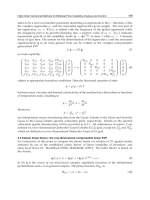
Concurrent Subspace Optimization for Aircraft System Design

271
When X
i*
is the optimal solution vector for the single objective optimization of the ith
objective function J
i
, the utopia point and pseudo nadir point are defined as







Utopia
1* 2* m*
12 m
,,,JJJ J





XX X (17)

Nadir Nadir Nadir Nadir
12 m
,,,JJJ J





 (18)

Where






Nadir 1* 2* m*
max
iiii
JJJJ





XX X
and m is the number of objective
functions.

Then with a large step size of the weighting factor the usual weighted sum method is used
in the variant of GSECSSO to approximate the Pareto front quickly. The subspace
optimization for AWSCSSO can be expressed as














11 1 1 2 22 1 11 2 22 2 1 2
01 01
1112 1 1 12 1 2
02 02
21 2 1 2212 2 2
1112 2221
Sub-optimization 1 Sub-optimization 2
ˆˆ
ˆˆ
Min , , Min , ,
ˆˆ
s.t. , , 1 s.t. 1
ˆˆ

1,,1
ˆˆ
,,
WF WF WF WF
CCrCCr
CCr C Cr
ff

 
 

X
YY X X X YY
XYY X
XXYY
YXY YXY

3
ˆ
,Y
(19)
Where the value with symbol ‘^’ above is a linearly approximated one, C
1
and C
2
are
cumulative constraints of G
1
and G
2

, respectively, and
p
k
r represents responsibility assigned
to the k-th subsystem for reducing the violation of C
p
. The value with superscript ‘
0
’ is
corresponding to the starting point X
0
. W
1
and W
2
are weighting factors for objective
function vector F
1
and F
2
, respectively.
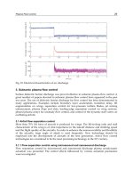
By estimating the size of each Pareto patch, the refined regions in the objective space are
determined. An example of the mesh refinement in AWSCSSO is shown in Fig. 9. Where
hollow points represent the newly refined node P
E
(expected solution) while solid points
represent initial four nodes that define the patch. As shown in Fig. 9, the quadrilateral patch
is taken as an example. If the line segment that connects two neighboring nodes of the patch
is too long, it is divided into only two equal line segments. The central point becomes the

P
1
P
2
P
3
P
4
P
E
P
5
P
6

Fig. 9. Refine patches of AWSCSSO method

Aeronautics and Astronautics

272
new refined node. These refined nodes are connected to form a refined mesh. Then the
sub-optimizations in Eq. (19) are performed using different additional constraints for
different refined nodes and the new Pareto points are obtained. In next step, according to
the prescribed density of Pareto points, the Pareto-front patch that is too large will be
refined again in the same way. In subsequent steps, the refinement and sub-optimizations
are repeated until the number of Pareto points does not increase anymore.
2.
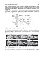
In the subsequent stage only these regions are specified as feasible domains for sub-
optimization problem with additional constraints. Each Pareto front patch is then
refined by imposing additional equality constraints that connect the pseudo nadir point

(P
N
) and the expected Pareto optimal solutions (P
E
) on a piecewise planar surface in the
objective space (as shown in Fig. 10).

1
F
2
F
Pseudo Nadir Point
P
1
P
2
E
P
E
P
A
P
Pseudo Nadir Point
P
1
P
2
P
3
P

4
3
F
2
F
1
F
N
P
A
P
2

N
P
Unknown Pareto Front

a) 2-D representation b) 3-D representation
Fig. 10. AWSCSSO method for multidimensional problems
Sub-optimizations are defined by imposing additional constraint H to Eq. (19) as















11 1 1 2 22 1 11 2 22 2 1 2
01 01
1112 1 1 12 1 2
02 0
21 2 1 2212 2
1112
112
Sub-optimization 1 Sub-optimization 2
ˆˆ
ˆˆ
Min , , Min , ,
ˆˆ
s.t. , , 1 s.t. 1
ˆˆ
1,,1
ˆ
,
ˆ
,, 0
WF WF WF WF
CCrCCr
CCr C C
f
H

 

 


X
YY X X X YY
XYY X
XXYY
YXY
XYY



2
2
22213
213
ˆˆ
,,
ˆˆ
,, 0
r
f
H



YXYY
XYY
(20)
The additional inequality constraint is







EN N
EN N
L0H
 



FF FXF
FFFXF
(21)
Where L is the adaptive relax factor that is less than 1.
E
F
,
N
F
and

F
X are the
normalized position vector of node P
E
, P

N
and the current design point X respectively. In

Concurrent Subspace Optimization for Aircraft System Design

273
AWSCSSO, L is set to be increased with the rise of the distribution density of Pareto
points.
Fig. 11 shows the framework of AWSCSSO. In Fig. 11, W
1i
and W
2i
are weighting factors in
stage 1 and stage 2, respectively; H is the additional constraint. The optimization problem is
performed in two stages in the AWSCSSO method. In the first stage the Pareto front is
approximated quickly with large step size of weight factors. The optimization problems of
this stage are defined in Eq. (19). In the subsequent stage, by calculating the distances
between neighboring solutions on the front in objective space, the refined regions are
identified and the refined mesh is formulated. Only these regions then become the feasible
regions for optimization by imposing additional constraints in the objective space. The
optimization problems of this stage are defined in Eq. (20). The different locations of new
Pareto points are defined by the different additional constraints. Optimization is performed
in each of the regions and the new solution set is acquired. Being a MDO problem, the
optimization is performed by the variant of GSECSSO method.

Stage 1: Acquire several control point to define a rough profile of the
Pareto front.
Sub-optimization using CSSO Sub-optimization using CSSO
W
11

CSSO optimization
Subspace
optimization
Subspace
optimization

System-level
coordination

Stage 2: Regions defined by refine nodes are specified as feasible
domains for sub-optimization by assigning additional constraints.
Sub-optimization using CSSO Sub-optimization using CSSO

Refine Pareto front patches
HH
W
12
W
21
W
22
Process Flow
Calling CSSO optimization

Fig. 11. Framework of AWSCSSO method
4.4 Examples
4.4.1 Example 1: Convex Pareto front
This problem is taken from a test problem (Huang, 2003). This is a test problem available
in the NASA Langley Research Center MDO Test Suite. It has two objectives, F
1

and F
2
, to
be minimized. It consists of ten inequality constraints, four coupled state variables and ten
design variables in two coupled subsystems. The mathematical model is not listed here
for concision. We refer the readers to the test problem 1 in the corresponding references.
The comparison of the solution obtained by MOPCSSO and AWSCSSO is shown in Fig. 12.
It can be concluded that for the problem with convex Pareto front a uniformly-spaced wide-
distributed and smooth Pareto front can be obtained by AWSCSS method. When using
MOPCSSO I have not captured the whole range.

Aeronautics and Astronautics

274
-300 -200 -100 0 100 20
0
-300
-200
-100
0
100
200
AWSCSSO
MOPCSSO
F
2
F
1

Fig. 12. Comparison of Pareto front obtained by using AWSCSSO and MOPCSSO

4.4.2 Example 2: Non-convex Pareto front
This problem consists of two objective functions, six design variables and six constraints.
Two objectives, F
1
and F
2
need to be minimized. The model problem is defined as

    














22
22 2
112345
222222
2123456
112
212

312
412
2
534
2
65 6
126 35 4
Min 25 2 2 1 4 1
Min
s.t. 2 0
60
20
230
43 0
340
0,,10,1,5,0 6
Fxxxxx
F xxxxxx
cxx
cxx
cxx
cxx
cxx
cx x
xxx xx x
 


  
  

  
   


x
x
x
x
x
x
x
x
(22)
-300 -200 -100 0
0
20
40
60
80
AWSCSSO
MOPCSSO
F
2
F
1

Fig. 13. Comparison of Pareto fronts obtained by using AWSCSSO and MOPCSSO methods

Concurrent Subspace Optimization for Aircraft System Design

275
The comparison of Pareto front obtained by AWSCSSO and MOPCSSO is shown in Fig. 13. It
is concluded that, for the problem with non-convex Pareto front, the more uniformly-spaced,
more widely-distributed and smoother Pareto front is also obtained by the AWSCSSO method.
4.4.3 Example 3: Conceptual design of a subsonic passenger aircraft
The mathematical model of this problem is defined as

C
d0L d0C
f
To L
To L
Max
Max
s.t. 0.2, 0.02
1
0.027, 0.024
1981, 1371
U
LD
CC
R
qq
DD




(23)
The objective functions in Eq. (23) are to maximize useful load fraction (U) and lift-to-drag

ratio for the cruising condition (L/D
C
). The constraints in Eq.(23) are as follows. (1) The drag
coefficient for the take-off condition and landing condition (C
d0L
) is no more than 0.2 and
that for the cruising condition (C
d0C
) is no more than 0.02. (2) The overall fuel balance
coefficient (R
f
) is no less than 1. (3) The achievable climb gradient for the take-off condition
(q
To
) is greater than 0.027 and that for the landing condition (q
L
) is greater than 0.024. (4) The
take-off field length (D
To
) is less than 1981m and the landing field length (D
L
) is less than
1371m. The overall fuel balance coefficient is defined as the ratio of the fuel weight required
for mission to that available for mission. The design variables are listed in Table 3.

Design Variable ⁄ unit Symbol Lower limit Upper limit
Wing area ⁄ m
2
S 111.48 232.26
Aspect ratio AR 9.5 10.5

Design gross weight ⁄ 10
3
kg W
d
g
63.504 113.400
Installed thrust ⁄ 10
3
kg T
i
12.587 24.948
Table 3. List of design variables
Two disciplines, aerodynamics and weight, are considered in this problem. The dataflow
between and in subsystems is analyzed in Fig. 14, where L/D
To
, L/D
L
, L/D
C
are the lift-to-
drag ratios for the take-off, landing and cruising conditions respectively, V
br
is the cruise
velocity with the longest range, R
fr
is the fuel weight fraction required for mission, and C
d0C

is the zero-lift drag coefficient for the cruising condition.
Two disciplines, aerodynamics and weight, are coupled. When the state variables in

aerodynamics such as cruise velocity with the longest range, lift coefficients, zero-lift drag
coefficients, skin-friction drag coefficients, lift-to-drag ratio are computed, some state
variables in Weight such as R
fr
should be known. Similarly, when the state variables in
Weight such as useful load fraction, overall fuel balance coefficient, achievable climb
gradient on take-off and landing, take-off field length and landing field length are
computed, some state variables in Aerodynamics such as L/D
To
, L/D
L
, L/D
C
and V
br
should
also be provided. In the Aerodynamics discipline, V
br
is coupled with C
d0C
. The dataflow
between state variables and design variables can be seen in Fig. 15. Many details of
equations in the aerodynamic discipline model and weight discipline model can refer to the

Aeronautics and Astronautics

276
reference (Zhang et al., 2008). The full description of them can be found in the references
(Lewis & Mistree, 1995; Lewis, 1997).

Aerodynamics
Aerodynamics
Weight
fr
R
br
To L C
,,,LD LD LD V
br
V
d0C
C

Fig. 14. Dataflow between and in subspaces

br
V
dg
W
C
LD
To
LD
L
LD
fr
R
f
R
U

To
q
L
q
To
D
L
D
i
T
S
AR

Fig. 15. Dataflow between state variables and design variables

20.7 20.8 20.9 21.0 21.1
0.46
0.47
0.48
0.49
0.50
0.51
0.52
U
L/D
C

Fig. 16. Pareto front obtained by using AWSCSSO

Concurrent Subspace Optimization for Aircraft System Design

277
The Pareto front obtained using AWSCSSO is shown in Fig. 16. Each solution on Pareto
front is obtained using CSSO with iterative subspace optimizations. Taking one of the
optimal designs as example, the values of the design variables are: S=232.3m
2
, AR=10.5,
W
dg
=113.4×10
3
kg, T
i
=16.75×10
3
kg. The performance parameters of the aircraft in optimal
design are as follows: C
d0C
=0.01777, L/D
C
=21.05, V
br
=183.43m/s, q
To
=0.03303, q
L
=0.08804,
D
To
=1823m and D

L
=1086m. Several conclusions can be made from these results. 1) The
AWSCSSO method is primarily proved to be applicable for aircraft conceptual design. 2)
The distribution of Pareto points is not so uniform as expected. These results are still very
encouraging in general. The non-uniformity may be due to the additional constraint that
changes the location to expected solution. Further study is still needed on how to achieve
the balance between uniformity and convergence.
5. Conclusion
The CSSO method is one of the main bi-level MDO methods. Couples of CSSO methods for
single- and multi-objective MDO problems are discussed in this chapter. It can be concluded
that, (1) number of the system analysis can be greatly reduced by using the CSSO methods,
which in turn improve the efficiency; (2) the CSSO methods enable concurrent design and
optimization of different design groups, which can greatly improve efficiency; (3) the CSSO
methods are effective and applicable in solving not only single-objective but also multi-
objective MDO problems.
For the CSSO methods, although the RSCSSO method behaves more robust, it will actually
reduce to a single-level surrogate modeling based MDO method since the subspace
optimizations have little impact on the results. So the GSECSSO method is more promising
as a bi-level method and worth further studying. The future study on the GSECSSO method
will focus on improving its robustness and efficiency. For the multi-objective CSSO
methods, the AWSCSSO method behaves better on obtaining widely-distributed Pareto
points. The future work on the multi-objective CSSO methods will focus on improving the
solution quality and also on testing it for more realistic engineering design problems.
6. References
Aute, V. and Azarm, S. A, “Genetic Algorithms Based Approach for Multidisciplinary
Multiobjective Collaborative Optimization,” 11th AIAA/ISSMO Multidisciplinary
Analysis and Optimization Conference, Virginia, 2006, AIAA 2006-6953.
Azarm, S. and Li, W.C., “Multi-level Design Optimization using Global Monotonicity Analysis,”
ASME Journal of Mechanisms and Automation in Design, 1989, Vol.111, No.2, pp.259-263.
Bolebaum, C.L., “Formal and Heuristic System Decomposition in Structural Optimization,”

NASA-CR-4413, 1991.
Huang, C. H., “Development of Multi-Objective Concurrent Subspace Optimization and
Visualization Methods for Multidisciplinary Design,” Ph.D. Dissertation, The State
University of New York, New York, 2003.
Huang, C. H. and Bloebaum, C. L., “Incorporation of Preferences in Multi-Objective
Concurrent Subspace Optimization for Multidisciplinary Design,” 10th
AIAA/ISSMO Multidisciplinary Analysis and Optimization Conference, New York,
2004, AIAA 2004-4548.
Huang, C. H. and Bloebaum, C. L., “Multi-Objective Pareto Concurrent Subspace Optimization
for Multidisciplinary Design,” AIAA Journal, Vol. 45, No. 8, 2007, pp. 1894-1906.

Aeronautics and Astronautics

278
Kreisselmeier, G., Steinhauser, R., "Systematic Control Design by Optimizing a Vector
Performance Index," IEAC Symposium on Computer Aided Design of Control Systems,
Zurich, Switzerland, 1979.
Kim, I. Y. and de Weck, O. L., “Adaptive Weighted Sum Method for Multiobjective
Optimization,” 10th AIAA/ISSMO Multidisciplinary Analysis and Optimization
Conference, New York, 2004, AIAA 2004-4322.
Kim, I. Y. and de Weck, O. L., “Adaptive Weighted-sum Method for Bi-objective
Optimization: Pareto Front Generation,” Structural and Multidisciplinary
Optimization, No. 29, 2005, pp. 149-158.
Lewis, K., Mistree, F. “Designing Top-level Aircraft Specifications-A Decision-based
Approach to A Multiobjective, Highly Constrained Problem,” 6th
AIAA/USAF/NASA/ISSMO Symposium on Multidisciplinary Analysis and
Optimization, Bellevue, WA, AIAA 1995-1431.
Lewis, K., “An Algorithm for Integrated Subsystem Embodiment and System Synthesis,”
Ph.D. Dissertation, Georgia Institute of Technology, Atlanta, Georgia, August 1997.
McAllister, C. D., Simpson, T. W. and Yukesh, M. “Goal Programming Applications in

Multidisciplinary Design Optimization,” 8th AIAA/USAF/NASA/ISSMO Symposium
on Multidisciplinary Analysis and Optimization, CA, 2000, AIAA 2000-4717.
McAllister, C. D., Simpson, T. W., Lewis, K. and Messac, A., “Robust Multiobjective
Optimization through Collaborative Optimization and Linear Physical
Programming,” 10th AIAA/ISSMO Multidisciplinary Analysis and Optimization
Conference, New York, 2004, AIAA 2004-4549.
Orr, S. A. and Hajela, P., “Genetic Algorithm Based Collaborative Optimization of A Tilrotor
Configuration,” 46th AIAA/ASME/ASCE/AHS/ASC Structures, Structural Dynamics
& Materials Conference, Texas, 2005, AIAA 2005-2285.
Parashar, S. and Bloebaum, C. L., “Multi-objective Genetic Algorithm Concurrent Subspace
Optimization (MOGACSSO) for Multidisciplinary Design,” 47th AIAA/ASME/
ASCE/AHS/ASC Structures, Structural Dynamics, and Materials Conference, Rhode
Island, 2006, AIAA 2006-2047.
Renaud, J.E. and Gabriele, G.A., “Second Order Based Multidisciplinary Design
Optimization Algorithm Development,” Advance in Design Automation, 1993, Vol.65,
No.2, pp.347-357.
Renaud, J.E. and Gabriele, G.A. “Improved coordination in non-hierarchic system
optimization,” AIAA Journal, 1993, Vol.31, No.12, pp.2367-2373.
Renaud, J.E. and Gabriele, G.A., “Approximation in non-hierarchic system optimization,”
AIAA Journal, 1994, Vol.32, No.1, pp.198-205.
Sellar, R. S, Batill, S. M and Renaud, J. E., “Response surface based, concurrent subspace
optimization for multidisciplinary system design,” 34th AIAA Aerospace Sciences
Meeting, 1996, AIAA 96-0714.
Sobieszczanski-Sobieski, J., “Optimization by Decomposition: A Step from Hierarchic to
Non-hierarchic Systems,” Recent Advances in Multidisciplinary Analysis and
Optimization, NASA CP-3031, Hampton, 1988.
Sobieszczanski-Sobieski, J., “Sensitivity of Complex, Internally Coupled Systems,” AIAA
Journal, Vol. 28, No. 1, 1990, pp. 153-160.
Tappeta, R. V. and Renaud, J. E., “Multiobjective Collaborative Optimization,” ASME
Journal of Mechanical Design, No. 3. 1997, pp. 403-411.

Zhang, K.S., Han, Z.H., Li, W.J., and Song, W.P., “Bilevel Adaptive Weighted Sum Method
for Multidisciplinary Multi-Objective Optimization,” AIAA Journal, 2008, Vol.46
No.10, pp. 2611-2622.
10
The Assessment Method for
Multi-Azimuth and Multi-Frequency
Dynamic Integrated Stealth
Performance of Aircraft
Ying Li, Jun Huang, Nanyu Chen and Yang Zhang
Beijing University of Aeronautics and Astronautics, Beijing,
China
1. Introduction
Stealth technology of aircraft, known as one of the three technological revolutions together
with high-energy laser weapons and cruise missiles in the development history of military
science since 1980s, has become the third milestone after jet engines and swept wings
technology in modern aviation history. Stealth aircraft has been also considered as one of
the ten greatest inventions of the U.S. ADARPA (Defense Advance Research Project
Agency). Nowadays, stealth technology has become one key technology. The countries all
over the world have paid great attention and strived to develop the stealth technology.
Reasonable assessment method for stealth performance plays a crucial role in the
development of advanced stealth technology. For example, the result of the stealth
performance assessment of aircraft can provide reference for modifying the aircraft’s stealth
design to achieve a higher stealth performance. Meanwhile, it can also provide reference for
making some specific strategies to increase the probability of successful tasks by reducing
the detecting probability of the radar or radar network. Nowadays, the electronic battlefield
is becoming more complex and it is urgent to build up a new method to analyze the multi-
azimuth and multi-frequency dynamic integrated stealth performance of aircraft, under the
complex electronic environment.
The existing stealth performance assessment methods include two types. One is the static
stealth performance assessment method, the other is the stealth assessment method based

on the effectiveness of combat simulation. The former just uses the average RCS value of
target circumferential area, or that of some critical radar detecting areas, under some
important radar frequencies as the basis. And the latter uses aircraft’s survival probability
(including detection probability, hitting probability and damage probability) in specific
combat tasks as the basis to assess the stealth performance of aircraft. Each method can
reflect the characteristics of the target’s stealth performance well. However, there are still
some limitations such as: the results based on the two methods can’t reflect the impact on
aircraft stealth performance caused by different target scattering characteristics. As not
taking the certain combat task and detecting environment into consideration, the results also
fail to reflect the dynamic characteristics of stealth performance, which happens in the entire

Aeronautics and Astronautics

280
proceeding of different combat tasks of aircraft, and the multi-azimuth and multi-frequency
integrated stealth performance under complex electronic environment. According to the
above, the development of modern stealth technology urgently requires a new type of
stealth performance assessment method to provide the reliable basis.
In this paper, a new type assessment method for multi-azimuth and multi-frequency
dynamic integrated stealth performance of aircraft was established by building the multi-
azimuth and multi-frequency dynamic integrated stealth performance assessment models
and the series of assessment criteria. With these efforts, on the one hand, a more reasonable
analysis result of stealth performance based on the multi-azimuth and multi-frequency
dynamic detecting environment can be provided, on the other hand, the limitations of the
existing stealth performance assessment methods can be overcame.
2. The existing stealth performance assessment method
Although lots of countries home and abroad started researches about the stealth
technology early, there are just only a few assessment methods for stealth performance of
aircraft. One of the two main existing methods is static stealth performance assessment
method, the other is the stealth performance assessment method based on the

effectiveness of combat.
2.1 The static stealth performance assessment method
2.1.1 The theory of the static stealth performance assessment
The classical static stealth performance assessment method includes two aspects: one is
the static testing assessment method and the other is theoretical calculation assessment
method. The American scholar Knott E.F has made a number of deep studies into the
radar cross section calculation and testing technologies. Chinese scholars, such as
Ruanying Zheng, Kao Zhang, Dongli Ma and so on, also have done researches on radar
cross section calculation and testing, they propose the concept of critical RCS reduction
region of aircraft, which has been widely used. At present, the radar cross section testing
technology home and abroad has been used widely. The static radar cross section testing
is a method, by doing the outfield or laboratory RCS testing on made full-scale models or
reduce-scale models to get a basic understanding of the target scattering characteristics.
The existing methods of the radar cross section theoretical calculation mainly include
three types and they are the high frequency approximation, finite difference time domain
and finite difference time domain.
The detailed steps of static stealth performance assessment are as follows: First of all,
obtaining the RCS curve of the target under different radar detecting frequencies through
static testing method or theoretical calculation method, then analyzing the stealth
performance of aircraft, according to the average RCS of target circumferential area, or that
of some critical radar detecting area, or the RCS value of certain radar detecting azimuth,
under some important radar frequencies.
The assessment criteria of the static stealth performance assessment method is that the lower
the average RCS of target circumferential area, or that of some critical radar detecting area,
or the RCS of specific azimuth, under some important radar frequencies, the better the
stealth performance of aircraft has. Technology flow chart of the static stealth performance
assessment method is shown as Fig.1.
The Assessment Method for Multi-Azimuth and
Multi-Frequency Dynamic Integrated Stealth Performance of Aircraft

281





Fig. 1. Flow Chart of Static Stealth performance Assessment Method
The overall average RCS of both model one and model two is 0.5㎡. There are three RCS
curve peaks at
30

and
180

azimuth for model one. The maximum value of RCS curve
peak is 10 ㎡ and the azimuth-width is 4°. There are four RCS curve peaks at
45

,
135

and
225

azimuth. The maximum value of RCS curve peak is 20㎡ and its peak
azimuth takes up 4° as well.
A penetration testing is carried out in this section. The locations of every single radar in the
radar network and the penetration destination are shown in Table 1, where GR means single
radar and Basement stands for the penetration destination. The penetration testing angle is
set from

0
60 to
0
60 and the interval angles is 5

.
RCS data processing
Stealth performance Assessment
Assessment Conclusion
(Satisfy the Stealth performance Index, Y / N?)
Agreement and Project Description of
target’s stealth performance assessment
Organization of Stealth
performance assessment
Theoretical analysis and
calculation of RCS
Data of theoretical calculation of RCS
Data of Static RCS testing
Static RCS ground
testing

Aeronautics and Astronautics

282

Fig. 2. Circumferential scattering distributions of model one


Fig. 3. Circumferential scattering distributions of model two

Name GR1 GR2 GR3 GR4 GR5 GR6 GR7 Basement
Longitude 119.6330 121.550 120.4830 121.5330 121.6170 121.05 121.9667 121.5
Latitude 23.5667 24.0667 22.70 25.0330 24.0167 25.0667 24.8 25.0
Table 1. Locations of Each Single Radar and the Penetration Destination
Fig.4 to Fig.7 just show several simulation results of these two models. The Y axis of the
testing diagram the FoundValue stands for the radar network detection results. When
FoundValue is equal to 0, it means that no target has been found by radar network. When
FoundValue is equal to 1, it means the target has been found. The X axis of the diagram the
Time stands for the time length of the penetration testing process. Fig (a) is the radar
detection results of simulation model one and Fig (b) is the radar detection results of
simulation model two.
The Assessment Method for Multi-Azimuth and
Multi-Frequency Dynamic Integrated Stealth Performance of Aircraft

283

(a) (b)
Fig. 4. Simulation results comparison of model one and model two (penetration angle -60°)


(a) (b)
Fig. 5. Simulation results comparison of model one and model two (penetration angle -45°)


(a) (b)
Fig. 6. Simulation results comparison of model one and model two (penetration angle 0°)

Aeronautics and Astronautics

284

(a) (b)
Fig. 7. Simulation results comparison of model one and model two (penetration angle 15°)
It can be seen from the results that although the overall average RCS of the two simulation
models is 0.5㎡, the dynamic stealth performance of these two models differs much from
each other. Such as it is shown in Fig.6 and Fig.7, the simulation model two would be
discovered earlier by radar network than the model one at the same penetration angle. After
the model two was discovered for the first time, it was lost by the radar network for a long
time, while the model one was detected continuously by radar network after its first being
found.
Above all, the static stealth performance assessment method still has some limitations.
Conclusions drawn from the tests are listed as follows:
1. Different circumferential scattering distribution can makes the aircraft has absolutely
different stealth performance, even if they have the same circumferential average RCS;
2. According to the stealth performance of aircraft with different circumferential scattering
distribution, the average RCS of aircraft requirement could be appropriately relaxed.
2.3 The assessment method based on the effectiveness of combat
Based on the radar simulation and target signal simulation technology, the steps of
assessment method based on the effectiveness of combat are listed: first of all, calculating
the aircraft survival probability during the whole combat mission, then summarizing the
effects of RCS characteristic on aircraft survivability and evaluating the stealth performance
of aircraft. The rules of this method are the aircraft with higher survivability has better
stealth performance. The assessment method based on aircraft effectiveness of combat has
been investigated early abroad. Ball R E made deep studies into the RCS reducing
technology which would improve the survivability of aircraft greatly. At the same time,
some software corporations abroad developed many kinds of analysis software that were
applied for analyzing survivability and vulnerability of aircraft. For example, several kinds
of software developed by SURVIAC center could quantitatively and comprehensively
evaluate the survivability and vulnerability of aircraft in the situation of one to one air
battle. In China there are a great deal of research about the effects of aircraft RCS on its

survivability have been done. For example, Zhang Kao and Ma Dongli proposed the method
of calculating the survivability of stealth aircraft that carries out given mission. Aimed at
analyzing the effects of reducing aircraft RCS on survivability of aircraft.
The Assessment Method for Multi-Azimuth and
Multi-Frequency Dynamic Integrated Stealth Performance of Aircraft

285
Assessment method based on the effectiveness of combat reflects the stealth performance of
aircraft carrying out the given mission, but still has some limitations: firstly, this method
couldn’t reflect the process and dynamic character of the stealth performance of aircraft
during the whole mission. For example, the target ‘flashing signal’ caused by the different
distributions of strong scattering source. Secondly, the assessment method based on the
survivability could not reflect the character of multi-azimuth and multi-frequency dynamic
comprehensive stealth performance of aircraft, and it also ignores characters of the multi-
azimuth and multi-frequency electronic detecting environment.
3. The multi-azimuth and multi-frequency dynamic integrated stealth
performance assessment method
Because of the limitations of the existing assessment method told in chapter 2, it should
build up a new assessment method for stealth performance of aircraft. This method could
evaluate the multi-azimuth and multi-frequency dynamic comprehensive stealth
performance of aircrafts, not just gives the evaluation conclusions based on the average RCS
of target circumferential area, or that of some critical radar detecting areas. The aircraft with
different scattering characteristic could meet requirements of different missions. In order to
evaluate the multi-azimuth and multi-frequency dynamic comprehensive stealth
performance of aircraft, it should build up the RCS scattering model and the multi-azimuth
and multi-frequency dynamic detecting environment model when the aircraft carries the
given mission, then make the assessment rules for analyzing the multi-azimuth and multi-
frequency dynamic comprehensive stealth performance of aircraft.
3.1 The multi-azimuth and multi-frequency dynamic comprehensive assessment
models

This section describes the building steps of the multi-azimuth and multi-frequency dynamic
comprehensive assessment models in detail, the assessment model includes the typical
complex dynamic detecting environment simulation model based on the given mission and
the RCS scattering model of aircraft.
3.1.1 The RCS scattering model of aircraft
In order to build a model that could reflect the RCS scattering character of aircraft and use
this model to analyze the stealth performance, we need to guarantee the accuracy of the
model.
Aircrafts executing different missions will encounter different detecting threat at different
azimuths from land, sea, air and space. And even if using the same detector with the same
working mode, the signal of aircraft the radar detected may still changes at any moment in
the mission. So the method of building reduced-scale model of aircraft and doing
experiments is considered. We can acquire the corresponding data for building up the
scattering model of aircraft. The RCS database should include the data of aircraft RCS at
different azimuths, under different frequencies. It is impossible to meet the needs of
building the database by the way of building model and testing it because of the limitation
of experiment condition. So the feasible way is to combine the data from both experiment
and theoretical calculating. Fig 8 shows the detailed steps.

Aeronautics and Astronautics

286

Fig. 8. Flow chart of building the RCS database


Fig. 9. Schematic illustration of the aircraft scattering model
The aircraft scattering model can be built up based on the adequate RCS data. The detailed
steps of building up the aircraft scattering model are showed as Fig.9. The coordinate
system in Fig.9 is defined just the same as aircraft body axes coordinate system for building



X
Y
Z
Front direction of aircraft
O
The direction of radar wave
The Assessment Method for Multi-Azimuth and
Multi-Frequency Dynamic Integrated Stealth Performance of Aircraft

287
up equation of motion, which follows the right-handed screw rule.

and

are two
parameters of radar detecting wave.

is defined as the angle between the project of radar
wave on the XOY plane and the X-axes.

is defined as the angle between the project of
radar wave on the YOZ plane and the Y-axes.

and

together decide the location of radar
wave in aircraft body axes coordinate system.
The planform of one aircraft scattering model is shown as Fig10. Fig11 shows the test RCS

curve of this model. We can see from the two figures that the model’s RCS scattering character
is consistent with experiment result which looks like a butterfly. This building method of the
RCS scattering model is feasible. The method of building a scattering model is an innovation,
which accurately reflects the RCS scattering character of the aircraft under different
frequencies. This method could be applied for analyzing different kinds of stealth aircraft.


Fig. 10. Planform of the Aircraft Scattering Model


Fig. 11. Circumferential Test RCS curve of Aircraft

Aeronautics and Astronautics

288
3.1.2 The typical complex dynamic detecting environment model
The typical detecting environment is different when the aircraft executes different missions.
So if we want to evaluate the multi-azimuth and multi-frequency dynamic comprehensive
stealth performance of aircraft, we must consider the typical complex detecting
environment. For example, when an aircraft is executing a penetration mission, the main
radar detecting thread is from the head or tail direction of aircraft.
The detection environment of warfare is becoming more complex, so it is extremely difficult
to describe it completely and accurately. By studying the performance of radar detection
systems, we can summarize the typical detection environment. Here are the main elements
to describe the typical complex and dynamic detection environmental model including two
types, one is the main tactical applications, such as (1) characters of the two sides of combat.
(2) Threat which the opposing sides may meet. (3) Interference and anti-interference
measures of the opposing sides. The other is the related information of electronic equipment
in typical detection environment, such as: (1) Number of detectors. (2) Spatial distribution of
detectors. (3) Density of the detectors (time domain). (4) Parameters of the detector’s signal.

(5) Frequency and scope of the detector’s signal. (6) The power of detector. (7) Working
mode of detector. Using these model parameters above, we can accurately describe the
typical complex dynamic detection environment when aircraft carries a specific mission.
3.2 The multi-azimuth and multi-frequency dynamic comprehensive stealth
assessment rules
As mentioned above, the existing assessments method is based on the average RCS of
aircraft. In order to make sure that the aircraft stealth performance assessments conclusions
are applicable, which can be used to guide the new type of stealth aircraft design and stealth
performance analysis, we should consider the specific tasks the aircraft carries. When
performing different tasks, the aircraft may encounter different typical detection
environment. So it is not reasonable to use the same stealth performance assessment rules.
Therefore, this section will establish the multi-azimuth and multi-frequency dynamic
integrated stealth performance assessment rules based on the given mission. Based on
specific combat mission, the assessment rules should be built up by analyzing various types
of detection threat the aircraft may encounter and the influence of the aircraft scattering
characteristic. Based on the conclusions got from the assessment rules above, we can
compare and analyze the stealth performance of different aircrafts which perform the same
task. The task-based aircraft multi-azimuth and multi- frequency dynamic integrated stealth
performance assessment rules should satisfy two conditions:
1. Assessment rules should reflect the character of specific tasks carried by aircraft. For
example, the stealth performance assessment rules for penetration aircraft should reflect
the character of penetration task firstly. In different stages of penetration task, the
influence of the aircraft survivability and successful mission probability is different. For
example, the first time when penetration aircraft is found by radar (or radar network)
decides how many times the aircraft would probably be attacked by enemy firepower.
When penetration aircraft was first discovered by radar network, the distance from the
penetration destination determines whether the plane could use the remote attack
weapon. Therefore, the establishment of penetration stealth performance assessment
rules should be combined with the penetration characters, so that the evaluation
conclusions reflect the differences of stealth performance among different aircraft when

executing penetration.
The Assessment Method for Multi-Azimuth and
Multi-Frequency Dynamic Integrated Stealth Performance of Aircraft

289
2. The conclusion got from the assessment rules should be able to reflect the scattering
character of aircraft. For example, during the process of penetration, aircraft mainly get
detecting thread from its front azimuth by various types of detectors in the enemy air
defense. If the aircraft goes through the first line of air defense system undetected and
continues to fly to the enemy's air defense system, it may also be detected by radars at
its two side azimuths. Therefore, when establishing stealth performance assessment
rules, we should focus on the stealth performance of the front and two side azimuths of
aircraft. The stealth performance of penetration aircraft is changing all the time.
Therefore, the assessment rules should not only combine with combat characteristics of
the penetration mission, but also need to consider the dynamic scattering character of
penetration aircraft.
4. The effects of different aircraft circumferential RCS scattering characters
The aircrafts with different circumferential scattering characters is suitable for different
combat missions, caused by various configuration design parameters. The stealth
performance evaluation conclusions of aircraft with different circumferential RCS scattering
characters can provide reference for a reasonable layout design of new type of aircraft. This
section will combine the multi-azimuth and multi-frequency dynamic comprehensive
assessment rules developed in chapter 3 to analyze and evaluate the aircrafts with different
circumferential RCS scattering characters.
4.1 The new target integrated circumferential RCS scattering model
4.1.1 The relevant model parameters
There are several requirements which the model should meet for the new analysis method:
1) quantified the overall and partial RCS scattering characters of target; 2) setting up the
relations between each different radar detecting areas; 3) controlling the RCS scattering
changing trends of model through inducing several model RCS scattering control

parameters. Considering that the RCS value can reflect the quantified target scattering
characters and the differences between the RCS values may up to the magnitude order for
the different target azimuth, the average RCS value of target circumferential area is
introduced as one of the RCS scattering characteristic parameters of model and the unit is
dBsm, and its symbol is
ave

.
The existing analysis method does not take the effects of the changing relations between
different important radar detecting region on the target stealth ability into account. For
example, the aircraft could be excellent in depth penetration mission, if it has lower RCS
value at the front azimuth and higher RCS values at other azimuths. Moreover, if the stealth
aircraft has lower RCS value at its two side azimuths compared with that for the rest
azimuths, it can carry out penetration mission with a smaller horizontal distance arriving at
the enemy bases. In order to build up the relations between different target important
detecting areas, the new analysis method uses the average RCS value of target front
important radar detect area as the basis. Furthermore, the average RCS values of another
radar detecting areas are introduced into the model as the target local RCS scattering
characteristic parameters and the corresponding symbols are
i

(i=0,1,…). The subscript i
represents the sequence of radar detecting areas. For describing the relations between the

Aeronautics and Astronautics

290
target front and other direction important radar detecting areas, the new model defines a set
of relational parameters. Their symbols are
i

k

(i = 0,1,…) and can be written as:

0
/
i
i
k





 (1)
where
0


represents the average RCS value of the target front important radar detecting
area.


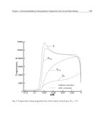
Fig. 12. RCS curve corresponding to one type of stealth aircraft (Under the S wave band).


Fig. 13. RCS curve corresponding to one type of aircraft (Under the S wave band).
The Assessment Method for Multi-Azimuth and
Multi-Frequency Dynamic Integrated Stealth Performance of Aircraft

291
Due to different stealth design parameters the UCAV X-45 and X-47 have, so they have
completely different RCS scattering characters. Their RCS curves differ much from each
other, as shown in Fig.12 and Fig.13. So the same set of RCS scattering controlling
parameters can not be used to describe the dissimilar RCS curve patterns and control the
RCS scattering changing trends of various new models well. There are two requirements for
the RCS scattering control parameters: one is that it is not advisable to introduce too many
RCS scattering control parameters, the other is the model can satisfy all kinds of stealth
ability analysis requirements. For example, building up the target circumferential RCS
scattering model with triangle pattern character as shown in Fig.2 needs two RCS scattering
control parameters, which can meet the requirements of controlling RCS scattering changing
trends and conducting target integrated stealth performance analysis. These parameters are
L
K and
A
K respectively,
L
K and
A
K can be expressed as:

/
Lab
KLL
(2)

/ 360
AF
KA


(3)
where
a
L and
b
L are the side lengths of model with triangle circumferential RCS scattering
character. The parameter
L
K can control the RCS scattering changing trends of target head
and tail areas. By this way, it can satisfy the analysis requirements about the effects of
different target head and tail stealth performance on its integrated stealth
performance.
F
A represents the angular region of target front important radar detecting area.
Likewise, the models with different
F
A
values can meet the analysis requirements about the
effects of different front important radar detecting areas on target integrated stealth
performance.


Fig. 14. RCS curves of different target RCS scattering models.

Aeronautics and Astronautics

292
Fig.14 shows the models with various target circumferential RCS scattering characters and
being built up by changing the values of
L

K and
A
K , when
ave

is equal to -10dBsm.
4.1.2 The model building method
According to Fig.12, the detailed building steps of the new model are described in this
section. First of all, defining the suitable target whole and local RCS scattering
characteristic parameters and introducing several model RCS scattering controlling
parameters according to the different target RCS scattering characters are necessary. So as
it is shown from Fig.1, the average RCS value of target circumferential area and the
heading direction within the angular region of
0
30 to
0
30 are introduced as the target
entire and local RCS scattering characteristic parameters respectively. Their
corresponding symbols are
ave

and
—
0
δ
.
L
K represents the ratio between long side and
short side lengths. Secondly, different functions are used to describe the RCS curves of
different radar detecting regions. The variable of curve function is angle value


, its
corresponding function value is length value R. But in the target RCS curve, the
corresponding value of angle

is the target RCS value. Therefore, a transform between
the coordinate length value R and the target RCS value is needed. Based on this
transform, RCS value in any direction of the target can be expressed by:

min
() ()
1
1
1
()
1
N
ave
ave i
N
i
i
i
RR
N
R
N








  


(4)

where
()
R

denotes the R value in any target azimuth,
i
R
is one of the series values of R
in any target important radar detecting areas and subscript i represents the sequence of
these R values,
ave

is the average RCS value of target circumferential area or local radar
detecting areas and
min

represents the RCS value of the coordinate origin. The stealth
analysis about the target local RCS scattering character should be included in the
conclusions of target integrated stealth performance analysis. So the last step is dividing
the target RCS curve into several parts according to the target RCS scattering characters,
then using different functions to describe these parts respectively. By this way, the

analysis conclusion about how the target local stealth performance affects its integrated
stealth ability can be reached. All the functions for every part of the curve can be written
as:

min
() () min
1
()
1
ave
N
i
i
R
R
N







 


(5)
where
()i



and
()i
R

are the target RCS values and R values respectively and corresponding
to the target azimuth of

. The subscript i represents the sequence of target important radar
detecting areas.
The functions corresponding to Fig.12 can be expressed as:
The Assessment Method for Multi-Azimuth and
Multi-Frequency Dynamic Integrated Stealth Performance of Aircraft

293

min min
()
min min
91
()
2cos
0
(180 ) (180 )
(360 ) 360
191
()
2sin
(180 ) (360 )
(360 ) 360

L
ave
Limit
Limit Limit
i Limit
ave
Limit Limit
Limit
K
Sum
or
or
Sum
or

 


 

 

 


 














 








(6)
90
01
1
2cos 2sin
Limit
Limit
L
K
Sum










where
ave

is the average RCS value of target circumferential area,
min

represents the RCS
value of the coordinate origin,

is the radar detect angle and
L
K is the model RCS
scattering controlling parameter.
4.2 Examples and discussions
In this section, the new kind of target circumferential RCS scattering models will be built
according to Fig.12 and Fig.13. Before that, disposing several radars in different azimuths
of enemy base. Combing relevant dynamic models and integrated stealth analysis rules
can give the detailed integrated stealth analysis conclusions. In these examples, aircraft
flight altitude is 1000m and flight velocity is 500m/s. The aircraft carries out the
penetration mission along a straight flight course at the azimuth of 90 degrees. The
azimuths of these radars are 0, 30, 45, 60, 90, 120, 135 and 180 degrees respectively. A
comparison is made between the integrated stealth performance of these two serial
models are given blow.

4.2.1 Rectangular RCS scattering models
Combining the new modeling methods described in Section 4.1.2 and the relevant stealth
performance analysis requirements, the serial models with absolutely different RCS
scattering characters are modeled.
The values of relevant model RCS scattering parameters are

ave
=-10dBsm and 0dBsm and
L
K
=0.5, 1.0 and 2.0 respectively. Fig.15 and Fig.16 compare the average radar detecting
probability of these serial models. Fig.15 shows that when
ave

is equal to -10dBsm, the RCS
scattering characters of these three models differs much from each other. Among these
models, the one corresponding to
L
K =0.5 has the highest average radar detecting
probability. When
L
K =1.0, the corresponding model will have much lower average radar
detecting probability. When
L
K = 0.5, the radars located in the two sides of the enemy base
will have much higher detecting probability than that for
L
K =1.0. So when
ave


is around -
10dBsm, the condition of
L
K =1.0 can make the penetration aircraft with rectangular RCS
scattering character have excellent sidewise stealth ability. Then the aircraft can carry out