Heat and Mass Transfer Modeling and Simulation Part 8 pot

Optimal Design of Cooling Towers

131
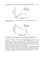
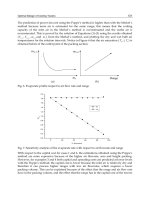
The prediction of power fan cost using the Poppe’s method is higher than with the Merkel´s
method because more air is estimated for the same range; this means that the cooling
capacity of the inlet air in the Merkel´s method is overestimated and the outlet air is
oversaturated. This is proved by the solution of Equations (1)-(3) using the results obtained
(
,win
T ,
,wout
T ,
,win
m and
a
m ) from the Merkel´s method, and plotting the dry and wet bulb air
temperatures for the solution intervals. Notice in Figure 6 that the air saturation (

wb a
TT) is
obtained before of the outlet point of the packing section.


(a) (b)
Fig. 6. Evaporate profile respect to air flow rate and range

0 20406080100
0.0
0.2
0.4

0.6
0.8
1.0
1.2
1.4
1.6
1.8
2.0
m
we
% decrease
R
m
a

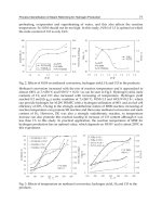
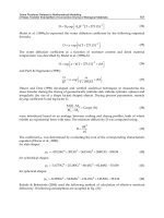
Fig. 7. Sensitivity analysis of the evaporate rate with respect to air flowrate and range
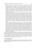
With respect to the capital cost for cases 1 and 6, the estimations obtained using the Poppe’s
method are more expensive because of the higher air flowrate, area and height packing.
However, for examples 3 and 4 both capital and operating costs are predicted at lower levels
with the Poppe’s method; the capital cost is lower because the inlet air is relatively dry and
therefore it can process higher ranges with low air flowrates, which requires a lower
packing volume. This can be explained because of the effect that the range and air flow rate
have in the packing volume, and the effect that the range has in the capital cost of the towers

Heat and Mass Transfer – Modeling and Simulation

132
(see Figure 8a, 8b and 8c). Notice in Figure 9 that there exists an optimum value for the
range to determine the minimum capital cost.

280 285 290 295 300 305 310
0
5
10
15
20
25
T
a
T
wb
280 285 290 295 300 305 310
0
5
10
15
20
25
T
a
T
wb

275 280 285 290 295 300 305 310
0
5
10
15
20
25

T
a
T
wb
275 280 285 290 295 300 305 310
0
5
10
15
20
25
T
a
T
wb

280 285 290 295 300 305 310
0
5
10
15
20
25
T
a
T
wb
280 285 290 295 300 305 310
0
5

10
15
20
25
T
a
T
wb

Fig. 8. Air temperature profile in the packing section

Optimal Design of Cooling Towers

133


Examples

1 2 3
Merkel Poppe Merkel Poppe Merkel Poppe
DATA
Q (kW) 3400 3400 3400 3400 3400 3400
T
a,in
(ºC)
22 22 17 17 22 22
T
wb,in
(ºC) 12 12 12 12 7 7
TMPI (ºC) 65 65 65 65 65 65

TMPO (ºC) 30 30 30 30 30 30
DTMIN (ºC)
10 10 10 10 10 10
w
in
(kg water/kg dry air) 0.0047 0.0047 0.0067 0.0067 0.0002 0.0002
RESULTS
T
w,in
(ºC) 50 38.8866 50 29.5566 50 45.4517
T
w,out
(ºC)
20 20 20 20 20 20
m
w,in
(kg/s) 25.720 29.9843 25.794 60.0479 25.700 22.1726
m
a
(kg/s) 31.014 43.2373 31.443 71.2273 28.199 31.4714
m
w,m
/m
a
(kg/s) 0.829 0.6824 0.820 0.8358 0.911 0.6897
m
w,r
(kg/s)
1.541 1.1234 1.456 1.0492 1.564 1.1268
m

w,e
(kg/s) 1.156 0.8425 1.092 0.7869 1.173 0.8451
T
a,out
(kg/s) 37.077 28.3876 36.871 23.3112 36.998 30.2830
Range (ºC)
30.00 18.8866 30.00 9.5566 30.00 25.4517
Approach (ºC) 8 8 8 8 13 13
A
fr
(m
2
) 8.869 10.1735 8.894 20.5291 8.862 7.4847
L
fi
(m) 2.294 1.2730 2.239 0.9893 1.858 1.0631
P (hP)
24.637 29.7339 24.474 25.6701 15.205 18.2297
Fill type Film Film Film Film Film Film
NTU 3.083 2.3677 3.055 1.6901 2.466 2.0671
Makeup water cost (US$/year)
23885.1 17412.4 22566.4 16262.7 24239.8 17465.3
Power fan cost (US$/year) 12737.6 32785.4 12653.7 13271.9 7861.0 9425.1
Operation cost (US$/year) 36622.7 32785.4 35220.0 29534.7 32100.8 26890.4
Capital cost (US$/year) 29442.4 29866.7 29384.6 42637.0 26616.0 23558.2
Total annual cost (US$/year) 66065.1 62652.1 64604.6 72171.7 58716.8 50448.6
Table 4. Results for Examples 1, 2 and 3

Heat and Mass Transfer – Modeling and Simulation

134


Examples

4 5 6
Merkel Poppe Merkel Poppe Merkel Poppe
DATA
Q (kW) 3400 3400 3400 3400 3400 3400
T
a,in
(ºC)
22 22 22 22 22 22
T
wb,in
(ºC) 12 12 12 12 12 12
TMPI (ºC) 55 55 65 65 65 65
TMPO (ºC) 30 30 25 25 30 30
DTMIN (ºC)
10 10 10 10 10 10
w
in
(kg water/kg dry air) 0.0047 0.0047 0.0047 0.0047 0.0047 0.0047
RESULTS
T
w,in
(ºC) 45 38.8866 50 24.1476 50 42.9877
T
w,out
(ºC)

20 20 15 15 25 25
m
w,in
(kg/s) 30.973 29.9843 22.127 59.2602 30.749 31.0874
m
a
(kg/s) 36.950 43.2373 32.428 85.9841 27.205 35.8909
m
w,m
/m
a
(kg/s) 0.838 0.6824 0.682 0.6824 1.130 0.8530
m
w,r
(kg/s)
1.547 1.1234 1.542 1.2539 1.540 1.0960
m
w,e
(kg/s) 1.160 0.8425 1.157 0.9404 1.155 0.8220
T
a,out
(kg/s) 34.511 28.3876 36.411 21.2441 39.083 30.6240
Range (ºC)
25.00 18.8866 35.00 9.1476 25.00 17.9877
Approach (ºC) 8 8 3 3 13 13
A
fr
(m
2
) 10.680 10.1735 7.630 20.2316 9.296 10.5566

L
fi
(m) 2.154 1.2730 6.299 3.0518 1.480 0.7831
P (hP)
26.852 29.7339 97.077 123.3676 10.754 10.9003
Fill type Film Film Film Film Film Film
NTU 2.293 2.3677 7.335 4.3938 1.858 1.4101
Makeup water cost (US$/year)
23983.4 17412.4 23901.7 19435.6 23865.9 16988.0
Power fan cost (US$/year) 13882.8 32785.4 50190.5 63783.4 5559.9 5635.7
Operation cost (US$/year) 37866.2 32785.4 74092.2 83218.9 29425.8 22623.7
Capital cost (US$/year) 32667.7 29866.7 43186.5 67320.6 25030.3 25202.8
Total annual cost (US$/year) 70533.9 62652.1 117278.7 150539.6 54456.0 47826.5
Table 5. Results for Examples 4, 5 and 6

Optimal Design of Cooling Towers

135


(a) (b) (c)
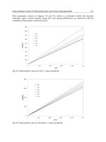
Fig. 9. Effect of range and air flow rate over packing volume and capital cost
For Examples 2 and 5, the designs obtained using the Merkel´s method are cheaper than
the ones obtained using the Poppe´s model; this is because the lower capital cost
estimation. In Example 2 there is a high inlet wet air temperature and therefore air with
poor cooling capacity, whereas in Example 5 there is a low outlet water temperature with
respect to the wet bulb air temperature, which reduces the heat transfer efficiency (see
Figure 10).
To demostrate that the Merkel´s method is less acurate, one can see cases 1 and 4, in which
the inlet air conditions are the sames but the maximum allowable temperatures are 50ºC and

45ºC. For the Merkel´s method the designs show the maximum possible range for each case;
however, the design obtained from the Poppe’s method are the same because the inlet air
conditions determine the cooling capacity.


285 290 295 300 305 310
2490000
2495000
2500000
2505000

T
wout
=288.15 K
T
wout
=293.15 K
i
masw
-i
ma
T
w


Fig. 10. Effect of the outlet water temperature over driving force

Heat and Mass Transfer – Modeling and Simulation

136

5. Conclusions
A mixer integer nonlinear programming model for the optimal detailed design of counter-
flow cooling towers has been presented. The physical properties and the transport
phenomena paramenters are rigorously modeled for a proper prediction. The objective
function consists of the minimization of the total annual cost, which considers operating and
capital costs. Results show that low wet temperatures for the air inlet and high ranges favor
optimal designs. The operating costs are proportional to the range, and the capital costs
require an optimal relation between a high range and a low air flow rate; therefore, the
strongest impact of the physical representation of the transport phenomenal is over the
capital cost. For all cases analyzed here the minimum possible area was obtained, which
means that the packing area is a major variable affecting the total annual cost. The cooling
capacity of the inlet air determines the optimum relation between range and air flowrate.
Since the model here presented is a non-convex problem, the results obtained can only
guaranty local optimal solutions. Global optimization techniques must be used if a global
optimal solution is of primary importance.
6. Appendix A
The relationships for physical properties were taken from Kröger [25]. All temperatures are
expressed in degrees Kelvin. The enthalpy of the air-water vapor mixture per unit mass of
dry-air is:







273.15 273.15 
ma a a fgwo v a
icpT wi cpT (A.1)
The enthalpy for the water vapor is estimated from:



,
273.15 
vfgwo vww
ii cpT (A.2)
The enthalpy of saturated air evaluated at water temperature is:







,, , , ,
273.15 273.15
ma s w a w w s w fgwo v w w
icpT wicpT (A.3)
The specific heat at constant pressure is determined by:

31 4 723
1.045356 10 3.161783 10 7.083814 10 2.705209 10
 
  
a
cp x x T x T x T (A.4)
Specific heat of saturated water vapor is determined by:

3105136

1.3605 10 2.31334 2.46784 10 5.91332 10

 
v
cp x T x T x T (A.5)
The latent heat for water is obtained from:

632 23
3.4831814 10 5.8627703 10 12.139568 1.40290431 10

 
fgwo
ix xTTxT
(A.6)
The specific heat of water is:

321326
8.15599 10 2.80627 10 5.11283 10 2.17582 10

  
w
cp x x T x T x T (A.7)
The humidity ratio is calculated from:

Optimal Design of Cooling Towers

137


 


 
,
,
0.62509
2501.6 2.3263 273.15
2501.6 1.8577 273.15 4.184 273.15 1.005
1.00416
2501.6 1.8577 273.15 4.184 273.15


 











vwb
wb
wb t v wb
wb
wb
P
T

w
TTPP
TT
TT
(A.8)
The vapor pressure is:

10
z
v
P (A.9)


8.29692 1
4
273.16
10
273.16
4.76955 1
4
273.16 273.16
10.79586 1 5.02808log 1.50474 10 1 10
4.2873 10 10 1 2.786118312











   



 
 


 





T
T
zx
TT
x
(A.10)
7. Nomenclature
i
j
a
disaggregated coefficients for the estimation of NTU
A
fr

cross-sectional packing area, m
2
i
k
b disaggregated coefficients for the estimation of loss coefficient
c
1
-c
5
correlation coefficients for the estimation of NTU
CAP capital cost, US$/year
C
CTF
fixed cooling tower cost, US$
C
CTMA
incremental cooling tower cost based on air mass flow rate, US$
s/kg
C
CTV
incremental cooling tower cost based on tower fill volume,
US$/m
3

i
CTV
C disaggregated variables for the capital cost coefficients of cooling
towers
COP annual operating cost, US$/year
c

j
variables for NTU calculation
i
j
c disaggregated variables for NTU calculation
cp
a
specific heat at constant pressure, J/kg-K
cp
v
specific heat of saturated water vapor, J/kg-K
cp
w
specific heat of water, J/kg-K
cp
w,in
specific heat of water in the inlet of cooling tower, J/kg-K
cp
w,out
specific heat of water in the outlet of cooling tower, J/kg-K
cu
e
unitary cost of electricity, US$/kW-h
cu
w
unitary cost of fresh water, US$/kg
d
1
-d
6

correlation coefficients for the estimation of loss coefficient,
dimensionless
k
d variables used in the calculation of the loss coefficient

Heat and Mass Transfer – Modeling and Simulation

138
i
k
d disaggregated variables for the calculation of the loss coefficient
D
TMIN minimum allowable temperature difference, ºC or K
i
e coefficient cost for different fill type
H
Y
yearly operating time, hr/year
HP power fan, HP
i
fgwo
heat latent of water, J/kg
i
ma
enthalpy of the air-water vapor mixture per mass of dry-air, J/kg
dry-air
i
ma,s,w
enthalpy of saturated air evaluated at water temperature, J/kg
dry-air

i
v
enthalpy of the water vapor, J/kg dry-air
J
recursive relation for air ratio humidity
K
recursive relation for air enthalpy
K
fi
loss coefficient in the fill, m
-1
K
F
annualization factor, year
-1
K
misc
component loss coefficient, dimensionless
L
recursive relation for number of transfer units
L
fi
fill height, m
Lef Lewis factor, dimensionless
m
a
air mass flow rate, kg/s
mav
in
inlet air-vapor flow rate, kg/s

mav
m
mean air-vapor flow rate, kg/s
mav
out
outlet air-vapor flow rate, kg/s
m
w
water mass flow rate, kg/s
m
w,b
blowdown water mass flow rate, kg/s
m
w,d
drift water mass flow rate, kg/s
m
w,ev
mass flow rate for the evaporated water, kg/s
m
w,in
inlet water mass flow rate in the cooling tower, kg/s
m
w,m
average water mass flow rate in the cooling tower, kg/s
m
w,out
outlet water mass flow rate from the cooling tower, kg/s
m
w,r
makeup water mass flow rate, kg/s

NTU number of transfer units, dimensionless
n
cycle
number of cycles of concentration, dimensionless
P vapor pressure, Pa
P
t
total vapor pressure, Pa
P
v,wb
saturated vapor pressure, Pa
Q heat load, W or kW
T
a
dry-bulb air temperature, ºC or K
TAC total annual cost, US$/year
T
a,n
dry-bulb air temperature in the integration intervals, ºC or K
TMPI inlet of the hottest hot process stream, ºC or K
TMPO inlet temperature of the coldest hot process streams, ºC or K
T
w
water temperature, ºC or K
T
wb
wet-bulb air temperature, ºC or K

Optimal Design of Cooling Towers

139
T
wb,in
inlet wet-bulb air temperature in the cooling tower, ºC or K
T
wb,n
wet-bulb air temperature in the integration intervals, ºC or K
T
w,in
inlet water temperature in the cooling tower, ºC or K
T
w,out
outlet water temperature in the cooling tower, ºC or K
w mass-fraction humidity of moist air, kg of water/kg of dry-air
w
in
inlet humidity ratio in the cooling tower, kg of water/kg of dry-
air
w
out
outlet humidity ratio in the cooling tower, kg of water/kg of dry-
air
w
s,w
humidity saturated ratio, kg of water/kg of dry-air
7.1 Binary variables
y
k
used to select the type of fill
7.2 Greek symbols

Δ
P
t
total pressure drop, Pa
ΔP
vp
dynamic pressure drop, Pa
Δ
P
fi
fill pressure drop, Pa
Δ
P
misc
miscellaneous pressure drop, Pa

f
fan efficiency, dimensionless
ρ
in
inlet air density, kg/m
3
ρ
m
harmonic mean density of air-water vapor mixtures, kg/m
3
ρ
out
outlet air density, kg/m
3

7.3 Subscripts
a dry air
b blowdown water
d drift water
e electricity
ev evaporated water
f fan
fi packing or fill
fr cross-sectional
in inlet
j constants to calculate the transfer coefficient depending of the fill
type
k constants to calculate the loss coefficient depending of the fill
type
m average
ma air-vapor mixture
misc miscellaneous
n integration interval
out outlet
r makeup

Heat and Mass Transfer – Modeling and Simulation

140
s saturated
t total
v water vapor
vp velocity pressure
w water
wb wet-bulb temperature

7.4 Superscripts
i fill type, i=1, 2, 3
8. References
Brooke, A., Kendrick, D., Meeraus, A. & Raman, R. (2006). GAMS User’s Guide (edition),
The Scientific Press, USA.
Burden, R.L. & Faires, J.D. (2005). Numerycal Analysis (8th edition), Brooks/Cole
Publishing Company, ISBN 9780534392000, California, USA.
Chengqin, R. (2006). An analytical approach to the heat and mass transfer processes in
counterflow cooling towers. Journal of Heat Transfer, Vol. 128, No. 11, (November
2006), pp. 1142-1148, ISSN 0022-1481.
Cheng-Qin, R. (2008). Corrections to the simple effectiveness-NTU method for
counterflow cooling towers and packed bed liquid desiccant-air contact systems.
International Journal of Heat and Mass Transfer, Vol. 51, No. 1-2, (January 2008), pp.
237-245, ISSN 0017-9310.
Douglas, J.M. (1988). Conceptual Design of Chemical Processes, McGraw-Hill, ISBN
0070177627, New, York, USA.
Foust A.S.; Wenzel, L.A.; Clump, C.W.; Maus, L. & Anderson, L.B. (1979). Principles of
Unit Operations (2nd edition), John Wiley & Sons, ISBN 0471268976, New, York,
USA.
Jaber, H. & Webb, R.L. (1989). Design of cooling towers by the effectiveness-NTU Method.
Journal of Heat Transfer, Vol. 111, No. 4, (November 1989), pp. 837-843, ISSN 0022-
1481.
Kemmer, F.N. (1988). The NALCO water handbook (second edition). McGraw-Hill, ISBN
1591244781, New, York, USA.
Kintner-Meyer, M. & Emery, A.F. (1995). Cost-optimal design for cooling towers.
ASHRAE Journal, Vol. 37, No. 4, (April 1995), pp. 46-55. ISSN 0001-2491.
Kloppers, J.C. & Kröger, D.G. (2003). Loss coefficient correlation for wet-cooling tower
fills. Applied Thermal Engineering. Vol. 23, No. 17, (December 2003), pp. 2201-2211.
ISSN 1359-4311.
Kloppers, J.C. & Kröger, D.G. (2005a). Cooling tower performance evaluation: Merkel,

Poppe, and e-NTU methods analysis. Journal of Engineering for Gas Turbines and
Power, Vol. 127, No. 1, (January 2005), pp. 1-7, ISSN 0742-4795.
Kloppers, J.C. & Kröger, D.G. (2005b). A critical investigation into the heat and mass
transfer analysis of counterflow wet-cooling towers. International Journal of Heat
and Mass Transfer, Vol. 48, No. 3-4, (January 2005), pp. 765-777, ISSN 0017-9310.

Optimal Design of Cooling Towers

141
Kloppers, J.C. & Kröger, D.G. (2005c). Refinement of the transfer characteristic correlation
of wet-cooling tower fills. Heat Transfer Engineering, Vol. 26, No. 4, (May 2005).
pp. 35-41, ISSN 0145-7632.
Kröger, D.G. (2004). Air-Cooled Heat Exchangers and Cooling Towers. PennWell Corp., ISBN
978-0-87814-896-7, Tulsa, Oklahoma, USA.
Li, K.W. & Priddy, A.P. (1985). Power Plant System Design (first edition), John Wiley &
Sons, ISBN 978-0-471-88847-5, New, York, USA.
Merkel, F. (1926). Verdunstungskühlung. VDI Zeitchrift Deustscher Ingenieure, Vol. 70, pp.
123-128.
Mills, A. E. (1999). Basic Heat and Mass Transfer (2nd edition), Prentice Hall, ISBN
0130962473, N.J., USA.
Nahavandi, A.N.; Rashid, M.K. & Benjamin, J.S. (1975). The effect of evaporation losses in
the analysis of counterflow cooling towers. Nuclear Engineering and Design, Vol.
32, No. 1, (April 1975), pp. 29-36, ISSN 0029-5493.
Olander, D.R. (1961). Design of direct cooler-condensers. Industrial and Engineering
Chemistry, Vol. 53, No. 2, (February 1961), pp. 121-126, ISSN 0019-7866.
Oluwasola, O. (1987). A procedure for computer-aided design of water-cooling towers,
The Chemical Engineering Journal, Vol. 35, No. 1, (May 1987), pp. 43-50, ISSN 1385-
8947.
Osterle, F. (1991). On the analysis of counter-flow cooling towers. International Journal of
Heat and Mass Transfer, Vol. 34, No. 4-5, (April-May 1991), pp. 1313-1316, ISSN

0017-9310.
Ponce-Ortega, J.M.; Serna-González, M. & Jiménez-Gutiérrez, A. (2010). Optimization
model for re-circulating cooling water systems. Computers and Chemical
Engineering, Vol. 34, No. 2, (February 2010), pp. 177-195, ISSN 0098-1354.
Poppe, M. & Rögener, H. (1991). Berechnung von Rückkühlwerken. VDI-Wärmeatlas, pp.
Mi 1-Mi 15.
Roth, M. (2001). Fundamentals of heat and mass transfer in wet cooling towers. All well
known or are further development necessary. Proceedings of 12
th
IAHR Cooling
Tower and Heat Exchangers, pp. 100-107, UTS, Sydney, Australia, November 11-14,
2001.
Rubio-Castro, E.; Ponce-Ortega, J.M.; Nápoles-Rivera, F.; El-Halwagi, M.M.; Serna-
González, M. & Jiménez-Gutiérrez, A. (2010). Water integration of eco-industrial
parks using a global optimization approach. Industrial and Engineering Chemistry
Research, Vol. 49, No. 20, (September 2010), pp. 9945-9960, ISSN 0888-5885.
Serna-González, M.; Ponce-Ortega, J.M. & Jiménez-Gutiérrez, A. (2010). MINLP
optimization of mechanical draft counter flow wet-cooling towers. Chemical
Engineering and Design, Vol. 88, No. 5-6, (May-June 2010), pp. 614-625, ISSN 0263-
8762.
Singham, J.R. (1983). Heat Exchanger Design Handbook, Hemisphere Publishing
Corporation, USA.
Söylemez, M.S. (2001). On the optimum sizing of cooling towers. Energy Conversion and
Management, Vol. 42, No. 7, (May 2001), pp. 783-789, ISSN 0196-8904.
Söylemez, M.S. (2004). On the optimum performance of forced draft counter flow cooling
towers. Energy Conversion and Management, Vol. 45, No. 15-16, (September 2004),
pp. 2335-2341, ISSN 0196-8904.

Heat and Mass Transfer – Modeling and Simulation

142
Vicchietti, A.; Lee, S. & Grossmann, I.E. (2003). Modeling of discrete/continuous
optimization problems characterization and formulation of disjunctions and their
relaxations. Computers and Chemical Engineering, Vol. 27, No. 3, (March 2003), pp.
433-448, ISSN 0098-1354.
7
Some Problems Related to Mathematical
Modelling of Mass Transfer Exemplified of
Convection Drying of Biological Materials
Krzysztof Górnicki and Agnieszka Kaleta
Warsaw University of Life Sciences, Faculty of Production Engineering
Poland
1. Introduction
Drying is a widely used industrial process, consuming 7-15% of total industrial energy
production in the industrialized world (Dincer & Dost, 1996). Drying is one of the most
common and the oldest ways of biological materials preservation such as vegetables and
fruits. The main objective in drying biological materials is the removal of water in the solids
up to a certain level, at which microbial spoilage and deterioration chemical reactions are
greatly minimalized.
The most important aspect of drying technology is the mathematical modelling of the
drying processes and the equipment. Its purpose is to allow design engineers to choose the
most suitable operating conditions and then size the drying equipment and drying chamber
accordingly to meet desired operating conditions. Full-scale experimentation for different
products and systems configurations is sometimes costly or even not possible (Sacilik et al.,
2006).
Convection drying of biological products is a complex process that involves heat and mass
transfer phenomena between the airflow and the product. Mathematical modelling of the
drying process of vegetables, fruits and grass is especially difficult because of high initial
moisture content (80-95% w.b.) and occurrence of shrinkage during drying.
The course and time of drying process depend on drying conditions, on temperature and

moisture profiles developed during the drying process, and above all, on moisture
movement in the material. Moisture movement is governed by the properties, form and size
of the product and the type of moisture bond in the material (Sander et al., 2003). The major
factors affecting the moisture transport during solids drying can be classified as:
i. external factors: these are the factors related to the properties of the surrounding air
such as temperature, pressure, humidity, velocity and area of the exposed surface,
ii. internal factors: these are the parameters related to the properties of the material such
as moisture diffusivity, moisture transfer coefficient, water activity, structure and
composition, etc. (Dincer & Hussain, 2004).
The development of mathematical models to describe the drying process has been the topic
of many research studies for several decades (Sander et al., 2003). Presently, more and more
sophisticated drying models are becoming available, but a major question that still remains
is the accuracy of predictions of drying processes using mathematical models. It is highly

Heat and Mass Transfer – Modeling and Simulation

144
dependent on the completeness of the mathematical model and the relationships used to
describe heat and mass transfer phenomena of dried products. However, professional
literature provides insufficient information on the mathematical modelling of mass transfer
during drying of biological materials with a high initial moisture content. Therefore, the aim
of the present chapter was to discuss in detail the main problems related to description of
the drying process of such materials using differential transport equations.
2. Differential transport equations for drying
According to the theory of convection drying of bodies with sufficiently high initial
moisture content, the process of convection drying should proceed in the first period of
drying until the critical moisture content is reached. The factors that influence the drying
process in the first period of drying are the conditions of external heat and mass exchange in
the system: drying product and surrounding air movement. For the case when moisture
content of the body is less than its critical moisture content, the second period of drying

begins. The process is decided by internal conditions of mass exchange and inner diffusion
of water because the internal resistance to water transfer in the body is greater than the
external resistance to water transfer from the body (Pabis, 1999; Pabis & Jaros, 2002).
2.1 The first drying period
The course of the drying process at the first drying period is decided by external conditions
of mass transfer. In this period the rate of drying is determined by the following equation
(Pabis, 1999):



0
aA
s
hA
dM
-TTkconst
dt W L
(1)
Eq. (1) resulted from the assumption that all heat delivered to the solid being dried at the
first drying period is used for vaporizing water. The solution of Eq. (1) with the assumption
valid for the first period of drying


Awb
TT
(2)
with initial condition M(t=0)=M
0
and with assumption that all parameters on the right side
of Eq. (1) are constant is the linear model



 
0
M t kt M (3)
The linear model means the acceptance of the assumption that the shrinkage can be
neglected. Biological materials with a high initial moisture content undergo, however,
shrinkage and deformation during hot-air drying. When water is removed from such a
material, a pressure unbalance is produced between the inner of the material and the
external pressure, generating contracting stresses that lead to material shrinkage or collapse,
changes in shape and occasionally cracking of the product. Mayor and Sereno (2004) gave a
detailed physical description of the shrinkage mechanism and presented a classification of
the different models proposed to describe this behaviour in materials with high initial
moisture content undergoing drying. The models were classified in two main groups:
empirical and fundamental models. Empirical models are convenient and easy to use and
Some Problems Related to Mathematical Modelling
of Mass Transfer Exemplified of Convection Drying of Biological Materials

145
therefore they are mainly applied to drying models. Acceptance of the assumption that the
surface of dried body changes because of the shrinkage means that A
0
in Eq. (1) should be
replaced by A. The solution of such changed Eq. (1) with assumption (2), initial condition
M(t=0)=M
0
, equation






23
00
AV
AV
(4)
and with the use of shrinkage model (Pabis, 1999)




00
VM
1-b b
VM
(5)
is the model of the first drying period which takes into account drying shrinkage
















3
0
0
11b b
Mt M 1 kt
1b 3M 1b
(6)



0
0.85
b
1M
(7)
Replacing shrinkage model described with Eq. (5) by model proposed by Karathanos (1993)





n
00
VM
VM
(8)

gives the following model of the first drying period












332n
0
2n 3
0
2n - 3 kt 3M
Mt
3M
(9)
Eq. (4) means that the constancy of the body shape during drying is taken into
consideration. However, such a situation not always occur in the case of the drying of
biological materials with a high initial moisture content and thus the dependence Eq. (4)
should also, for this reason, be regarded as approximate. In this connection, the accuracy of
calculation of A can be improved by introducing into Eq. (4) an empirical coefficient n
1
1,
which changes Eq. (4) to (Pabis, 1999)





1
23n
00
AV
AV
(10)
and Eq. (6) (after substitution of 3n
1
/(3n
1
-2)=N) to
















N
0
0
11b b
Mt M 1 kt
1b NM 1b
(11)

Heat and Mass Transfer – Modeling and Simulation

146
The parameter k, which occurs in the models of the first drying period, determines the
initial drying rate.
2.2 The second period of drying
It can be accepted that the water movement inside the dried solid is only a diffusion
movement in the convection drying process of biological materials with a high initial
moisture content. Therefore the equation applied to the description of the second drying
period of biological materials takes the following form (Luikov, 1970):




2
M
DM
t
(12)
Certain simplifications were made in this equation. It was assumed that shape and volume
of dried particle do not change, and that water diffusion coefficient is constant. (The
discussion how to take into account shrinkage and changeability of the water diffusion

coefficient will be conducted in Section 2.3).
The following initial and boundary conditions can be adopted:
i.
the initial condition: the same moisture content at any point of dried material at the
beginning of the second drying period (material before drying is cut into small pieces
and therefore this assumption can be accepted)



c
t0
M M (13)
ii.
one of the three boundary conditions can be taken:

the boundary condition of the first kind means that the external resistance to mass
transfer is negligible (i.e., the surface of the solid is at equilibrium with the
surrounding air for the time considered) and therefore the moisture content on the
solid surface is equal to the equilibrium moisture content


e
A
M M (14)

the boundary condition of the second kind means that the mass (water) flux from
the surface of the solid is known for the time considered





A
A
Wft

(15)

the boundary condition of the third kind means that the mass (water) flux from the
surface of the solid is expressed in terms of moisture content difference between
the surface and the equilibrium moisture content





me
A
A
M
-D h M M
n
(16)
For the mass transfer at the surface of the biological materials with a high initial moisture
content being dried the first kind and the third kind boundary conditions are mostly used in
mathematical models of the drying process (Markowski, 1997).
Biological materials before drying are cut into small pieces, mostly slices or cubes. Therefore
Eq. (12) applied to the description of the second drying period of biological materials takes
the following form (Luikov, 1970):
Some Problems Related to Mathematical Modelling
of Mass Transfer Exemplified of Convection Drying of Biological Materials

147
for an infinite plane (slices):







2
2
cc
MM
D
t
x
t0;-R x R
(17)
for a finite cylinder (slices):












22
22
c
MM1MM
D
trr
rz
t0;0rR;hz h
(18)
for cubes:



 






  
222
222
112233
M MMM
D
t
xyz
t0;-R x R;-R

y
R;-R z R
(19)
The initial conditions (Eq. (13)) are following:
for an infinite plane




c
M x,0 M const. (20)
for a finite cylinder




c
M r,z,0 M const. (21)
for cubes




c
Mx,
y
,z,0 M const. (22)
The boundary conditions of the third kind (Eq. (16)) take following form:
for an infinite plane











c
mce
MR,t
DhMR,tM
x
(23)
for a finite cylinder







 



c
mc e

MR,z,t
DhMR,z,tM
r
(24)








M0,z,t
0, M 0,z,t
r
(25)






 



me
M r,h,t
D h M r,h,t M
z

(26)

Heat and Mass Transfer – Modeling and Simulation

148






Mr,0,t
0
z
(27)
for cubes











1
m1 e
MR,y,z,t

DhMR,y,z,tM
x
(28)







  



2
m2e
Mx,R,z,t
DhMx,R,z,tM
y
(29)












3
m3e
Mx,y,R,t
DhMx,y,R,tM
z
(30)
An analytical solution of: (i) Eq. (17) at the initial and boundary conditions given by Eqs.
(20) and (23), (ii) Eq. (18) at the initial and boundary conditions given by Eqs. (21) and (24)-
(27), and (iii) Eq. (19) at the initial and boundary conditions given by Eqs. (22) and (28)-(30)
with respect to mean moisture content as a function of time, take the following form
(Luikov, 1970):
for an infinite plane












e
2
ii
2
ce

i1
c
Mt-M
D
Bexp μ t
MM
R
(31)
where



2
iii
22 2
ii
2Bi 1
B;ctgμμ
Bi
μ Bi Bi μ

for a finite cylinder




















2
2
j,2
i,1
e
i,1 j,2
22
ce
i1j1
c
μ
μ
Mt-M
BB exp Dt
MM
Rh
(32)
where



 

22
i,1 j,2
22 2 22 2
i,1 i,1
j
,2
j
,2
i,1 i,1
j
,2
j
,2
2Bi 2Bi
BB
μ Bi Bi μμBi Bi μ
11
ctg μμ;ct
g
μμ
Bi Bi

for cubes














  





e
n,1 m,2 k,3
ce
n1m1k1
22 2
n,1 m,2 k,3
222
123
Mt-M
BB B
MM
μμ μ
exp Dt
RRR
(33)

Some Problems Related to Mathematical Modelling
of Mass Transfer Exemplified of Convection Drying of Biological Materials

149
where



2
n,1
22 2
n,1 n,1
2Bi
B
μ Bi Bi μ



2
m,2
22 2
m,2 m,2
2Bi
B
μ Bi Bi μ




2

k,3
22 2
k,3 k,3
2Bi
B
μ Bi Bi μ


n,1n,1m,2m,2k,3k,3
111
ctg μμ;ct
g
μμ;ct
g
μμ
Bi Bi Bi

and for a cubic geometry R
1
=R
2
=R
3
.
In the literature on drying boundary conditions of the first kind are almost always taken
into account (it is easier to obtain the solution using such boundary conditions) and like for
boundary conditions of the third kind the infinite series constitute appropriate solutions.
Several researches showed that for large drying times an analytical solution of Eq. (12) for
sphere at the appropriate initial condition and boundary condition of the first kind with
respect to mean moisture content, can be reduced to the first term of infinite series (Jayas et

al., 1991). Pabis et al. (1998) found the relationship between the optimum number of terms in
infinite series and Fourier number for sphere and stated that the optimum number of terms
increases with the decreasing value of Fo. González-Fésler et al., (2008) demonstrated that
for values of Fourier number Fo (Fo=Dt/R
c
2
)0.1 the mathematical solution for the finite
cylinder drying including only the first term of each infinite series represents 95% of the
complete solution, so that terms with n>1 could be neglected. The number of terms in
analytical solution of Eq. (12) for an infinite plane (at the appropriate initial condition and
boundary condition of the first kind with respect to mean moisture content) necessary for
calculating the moisture ratio MR with accuracy δ=4% is i=5 for the initial phase of drying
(Fo=0), whereas i=20 and i=193 are needed to achieve an accuracy of 1% and 0.1%
respectively. The accuracy was defined as 100(M

-M
i
)/M

, where M

and M
i
are the exact
and truncated solutions, respectively (Efremov et al., 2008).
2.3 Determination of the parameters necessary for using the models of the second
drying period
Knowledge of the value of the critical moisture content, equilibrium moisture content, water
(moisture) diffusion coefficient, mass transfer coefficient and Biot number is necessary for
using model of the second drying period.

The critical moisture content M
c
could be determined assuming the continuity of the drying
process. The continuity of the process required that when M is equal to M
c
, the drying rate
in the first and second period be equal, that is when (dM/dt)
I
=(dM/dt)
II
(Jaros & Pabis,
2006). Górnicki & Kaleta (2007a) used the drying rate and the temperature of the dried
particle as a criterion of division into the first and the second drying period. The modelling
of the second drying period following the first drying period requires introducing into Eqs.
(31), (32), and (33) structure of corrected drying time t minus t
c
, where t
c
is the drying time
to the critical moisture content.
Equilibrium moisture content represents the moisture content that the material will attain if
dried for an infinite time at a particular relative air humidity and temperature. The relation

Heat and Mass Transfer – Modeling and Simulation

150
between the material moisture content and the relative humidity in equilibrium with the
product at the same temperature used to reach the equilibrium is termed the sorption
isotherm (the equilibrium moisture content – equilibrium relative humidity relationship).
The sorption isotherms of biological and food materials are the sigmoid shape, under the

Brunauer classification (Brunauer, 1943) of type II. The existing isotherm equations can be
divided into two separate groups: (i) empirical or partly empirical equations using
exponential, power or logarithmic functions and (ii) equations with some theoretical basis
and/or their combinations (Blahovec, 2004). It turned out that at least seventy seven
isotherm equations are available in the literature (van den Berg & Bruin, 1981). The
commonly used equations for biological materials are: the Langmuir, Brunauer-Emmett-
Teller (BET), Iglesias-Chirife, the modified Henderson, Chen, Chung-Pfost, Halsey, Oswin,
and Guggenheim-Anderson-de Boer (GAB) (Rizvi, 1995). The problems related to fitting
abilities of the existing isotherm equations for biological materials and selecting the best
equations are still under discussion (Castillo et al., 2003; Furmaniak et al., 2007; Kaleta &
Górnicki, 2007; Timmermann et al., 2001).
The value of the equilibrium moisture content is relatively small (especially for low air
relative humidity) compared to M(t) or M
0
and therefore the dimensionless moisture content
(moisture ratio) MR=[M(t)-M
e
]/(M
0
-M
e
) for the whole process of drying could be simplified
to M(t)/M
0
(Doymaz & Pala, 2002; Zielinska & Markowski, 2007).
In biological materials with a high initial moisture content water can be transported by
water diffusion, vapour diffusion, Knudsen diffusion, internal evaporation and
condensation effects, capillary flow, and hydrodynamic flow. Often there is a mixture of
various transport mechanisms, and the contributions of the different mechanisms to the
total transport varies from place to place and changes as drying progresses (Bruin &

Luyben, 1980). Therefore the water diffusion coefficient in the model of the second drying
period describes the total transport of moisture and is called the effective diffusivity. The
values of moisture diffusion coefficient for biological materials reported in the literature
lie within the range of 10
-12
– 10
-8
m
2
s
-1
(mostly about 10
-10
m
2
s
-1
) (Doulia et al., 2000;
Maroulis et al., 2001). It is known that moisture diffusion coefficient depends strongly on
temperature (e.g. Cuningham et al., 2007; Garcia-Pascual et al., 2006; Kaymak-Ertekin,
2002) and often very strongly indeed on the moisture content (e.g. Maroulis et al., 2001;
Waananen & Okos, 1996) and on material structure (e.g. Ruiz-Cabrera et al., 1997).
Nevertheless, there is no diffusion theory that is sufficiently well formulated and verified.
Therefore the most commonly used method for determining the moisture diffusion
coefficient in biological materials is by fitting the diffusion-based drying equations to the
experimental data in the second drying period. It should be emphasized, however, that
moisture diffusion coefficient determined with this method is limited in application to the
diffusion-based drying equation from which it was calculated and to the moisture range
in which experiments were conducted (Pabis et al., 1998). In the case of shrinkage and
changeability of the water diffusion coefficient the coefficient is determined from the

diffusion-based drying equation applying the method of inverse problem (Jaros et al.,
1992; Górnicki & Kaleta, 2004).
In the literature concerning mathematical modelling of convection drying of biological
materials the value of the water diffusion coefficient is mostly considered as a constant. An
Arrhenius – type equation is sometimes used to describe the relationship between the
diffusion coefficient and temperature of dried material: