Biomass and Remote Sensing of Biomass Part 9 potx

Introduction to Remote Sensing of Biomass
151
about 40% of the converted energy for dark respiration. Therefore, the maximum
photosynthetic efficiency is:
100x0.50x0.80x0.28x0.60 = 6.70
This result applies to c
4
plants (so-called because their first product of photosynthesis is 4-
carbon sugar). For c
3
plants, like wheat and rice, the efficiency is lower due to photo-
respiration effects.
1.11 Remote sensing of radiation intensity
1.11.1 Solar constant
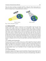
The average solar irradiance received outside the earth atmosphere is called Solar Constant.
The intensity of solar radiation above the earth's atmosphere has nearly constant value
unlike irradiance received at the ground. It's average value is 1367 W/m² though it shows
some variation due to variations in solar activity. Annual fluctuations due to Earth-Sun
distance give rise to a variation of ±3.4% of the extra-terrestrial irradiance and are given by
E
o
= <E
0
>(1 + 0.0167cos((2 /365)*(D-3)))²
where <E
0
> is the mean value of solar constant, D is the Julian days.
1.11.2 Radiation reflected and received by the ground
Radiation received at the ground surface is a combination of direct radiation, which comes
from the sun after passing through a path length in the transparent atmosphere, and diffuse

radiation which is radiation reflected by clouds and scattered by atmosphere in general. The
contribution of diffuse radiation to irradiance received by ground depends on the
atmospheric thickness, moisture content, cloud frequency, turbidity of the atmosphere, and
angle of zenith.
The radiation that is reflected from the ground is very small compared to that reflected from
the clouds. Its value depends on the reflectance of different earth surface features. In many
cases, surface albedo is taken to be uniform (0.15) across the land.
1.11.3 Atmospheric effects
Atmosphere plays a major role at attenuation and reflection of light that pass through it.
Their main effects are reflection, absorption, and scattering, depending on the wavelength
and air mass ratio.
1.11.4 Air mass ratio
Air mass ratio is defined as the ratio of the path length of the radiation through the
atmosphere at a given angle of a reference path length. The reference path length is that
obtained by light traveling to a point at sea level straight through the atmosphere
(vertically). The air mass ratio depends on the angle of zenith and the height above sea level
of the observer. For small angles, the ratio is expressed as;
m = sec θ
z
where θ
z
is the zenith angle. As the angle of zenith increases, the air mass ratio increases i.e.,
the attenuation increases.


Biomass and Remote Sensing of Biomass
152
1.11.5 Atmospheric absorption and reflection
Light passing through the atmosphere experiences absorption, scattering and reflection.
Absorption causes heating and eventual re-emission of the absorbed energy as long

wavelength radiation. Scattering is a wavelength dependent change in a direction. On the
average 30% extra-terrestrial irradiance is reflected to outer space mainly due to cloud.
1.11.6 Irradiance variation
Irradiance received at a given location may differ in magnitude from hour to hour, day to
day, month to month, and season to season depending on air mass, turbidity, moisture
content, cloud frequency, and angle of zenith. The seasonal variation give rise to a
significant amount of fluctuations in the irradiance received. This fluctuation in irradiance is
due to variation in the declination angle from season to season. The declination angle
(δ)
that the earth posses with respect to the sun varies from season to season. In the middle of
march and september the declination angle,
δ , is zero (0
o
), where as δ =23.5
o
and δ =-23.5
o

in the middle of June and December respectively. Analytically, the declination angle is
expressed as :


284
23.5 sin 360
365
o
D







where
D is the Julian days.
Depending on the latitude, for a given declination angle, the irradiance increases or
decreases. Moreover, irradiance varies with latitude. Irradiance variation due to seasonal
variation is great at high latitudes. Variation in the earth sun distance also contributes to the
variation in irradiance received although its contribution is very small.
2. Applications
2.1 Forestry applications
Satellite imagery is used to identify and map: -

The species of native and exotic forest trees.

The effects of major diseases or adverse change in environmental conditions.

The geographic extent of forests.
This application of satellite imagery has led to the extensive use of imagery by organizations
that have an interest in a range of environmental management responsibilities at a state and
national level.
2.1.1 Greenhouse gases — sinks and sources
Forests are often referred to as carbon sinks. This description is used because during
photosynthesis, carbon dioxide, the major greenhouse gas, is taken from the atmosphere
and converted into plant matter and oxygen.
Climate change has serious implications for Malaysia and overseas countries alike.
Sustainable v land management is essential for effective greenhouse gas management;
hence, it is important to acquire data on land cover in Malaysia. Remotely sensed land cover
changes are used in calculations of our national emission levels, and data collected on a
national scale will enable governments to develop responses to land clearing.

Introduction to Remote Sensing of Biomass
153
2.1.2 Vegetation health
Vegetation can become stressed or less healthy because of a change in a range of
environmental factors. These factors include lack of water, concentration of toxic
elements/herbicides and infestation by insects/viruses. The spectral reflectance of
vegetation changes according to the structure and health of a plant. In particular, the
influence of chlorophyll in the leaf pigments controls the response of vegetation to radiation
in the visible wavelength. As a plant becomes diseased, the cell structure of a plant alters
and the spectral signature of a plant or plant community will change. The maximum
reflection of electromagnetic radiation from vegetation occurs in the near infrared
wavelengths. Vegetation has characteristically high near-infrared reflectance and low red
reflectance. Air-borne scanners using narrow spectral bands between 0.4 urn and 0.9 urn can
indicate deteriorating plant health before a change in condition is visible in the plant itself.
2.1.3 Biodiversity
Vegetation type and extent derived from satellite imagery can be combined, with biological
and topographic information to provide information about biodiversity. Typically, this
analysis is done with a geographic information system.
2.1.4 Change detection
Satellite imagery is not always able to provide exact details about the species or age of
vegetation. However, the imagery provides a very good means of measuring significant
change in vegetation cover, whether it is through clearing, wildfire damage or
environmental stress. The most common form of environmental stress is water deficiency.
2.2 Geology
Remote sensing is useful for providing information relevant to the geosciences. For example,
remote sensing data are used in:

Mineral and petroleum exploration,


Mapping geomorphology, and

Monitoring volcanoes.
2.3 Land degradation
Imagery can be used to map areas of poor or no vegetation cover. A range of factors,
including saline or sodic soils, and overgrazing, can cause degraded landscapes.
2.4 Oceanography
Remote sensing is applied to oceanography studies. Remote sensing is used, for example, to
measure sea surface temperature and to monitor marine habitats.
2.5 Meteorology
Remote sensing is an effective method for mapping cloud type and extent, and cloud top
temperature. In many of the applications identified above remotely sensed data are used
with a range of other Earth science data to provide information about the natural
environment. This analysis of Earth science data from a range of sources is usually done in a
geographic information system (GIS).

Biomass and Remote Sensing of Biomass
154
2.6 Applications in agriculture, forestry, and ecology
2.6.1 General principles for recognizing vegetation
Planet Earth is distinguished from other Solar System planets by two major categories:
Oceans and Land Vegetation. The oceans cover ~70% of the Earth's surface; land comprises
30%. On the land itself, the first order categories break down as follows: Trees = 30%;
Grasses = 30%; Snow and Ice = 15%; Bare Rock = 18%; Sand and Desert Rock = 7%. We have
already seen in previous Sections and in the Overview that in false colour imagery the
remote sensing signature of vegetation is a bright red. The landscape shown in this first
image could almost be on Mars except for the presence of this bright red sign of vegetation.
This is the Ouargla Oasis in the Sahara Desert of southern Algeria, a concentration of trees
and plants where groundwater reaches the surface:

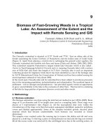
Fig. 16. Image of the Ouargla Oasis in the Sahara Desert of southern Algeria
On Earth, the amount of vegetation within the seas is huge and important in the food chain.
But for people the land provides most of the vegetation within the human diet. The primary
categories of land vegetation (biomes) and their proportions is shown in this pie chart:


Fig. 17. Pie chart for land vegetation (biomes) and their proportions
These biomes are defined in part by the temperature and precipitation controls that
differentiate them:

Introduction to Remote Sensing of Biomass
155

Fig. 18. Distribution of land vegetation by temperature and precipitation controls
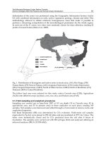
Global maps of vegetation biomes on the continents show this general distribution:


Fig. 19. Global maps of land vegetation (biomes)
A fair number of global vegetation maps have been published. These usually show slight to
moderate differences, depending in part with the types and numbers of classes established
in the classification. There also exists a notable correlation between vegetation classes and
climate. Remote sensing has proven a powerful "tool" for assessing the identity,
characteristics, and growth potential of most kinds of vegetative matter at several levels
(from biomes to individual plants). Vegetation behaviour depends on the nature of the
vegetation itself, its interactions with solar radiation and other climate factors, and the

Biomass and Remote Sensing of Biomass
156
availability of chemical nutrients and water within the host medium (usually soil, or water

in marine environments). A common measure of the status of a given plant, such as a crop
used for human consumption, is its potential productivity (one such parameter has units of
bushels/acre or tons/hectare, or similar units). Productivity is sensitive to amounts of
incoming solar radiation and precipitation (both influence the regional climate), soil
chemistry, water retention factors, and plant type. Examine the diagram below to see how
these interact, keeping in mind that various remote sensing systems (e.g., meteorological or
earth-observing satellites) can provide inputs to productivity estimation:


Fig. 20. Interaction between productivity and solar radiations


Fig. 21. Reflection and absorption of radiations through biomass

Introduction to Remote Sensing of Biomass
157
Because many remote sensing devices operate in the green, red, and near infrared regions of
the electromagnetic spectrum, they can discriminate radiation absorption and reflectance
properties of vegetation. One special characteristic of vegetation is that leaves, a common
manifestation, are partly transparent allowing some of the radiation to pass through (often
reaching the ground, which reflects its own signature). The general behaviour of incoming
and outgoing radiation that an act on a leaf is shown in figure 21.
Now, consider this diagram which traces the influence of green leafy material on incoming
and reflected radiation.


Fig. 22. The influence of green leafy material on incoming and reflected radiation.
Absorption centred at about 0.65 µm (visible red) is controlled by chlorophyll pigment in
green-leaf chloroplasts that reside in the outer or Palisade leaf. Absorption occurs to a
similar extent in the blue. With these colours thus removed from white light, the

predominant but diminished reflectance of visible wavelengths is concentrated in the green.
Thus, most vegetation has a green-leafy colour. There is also strong reflectance between 0.7
and 1.0 µm (near IR) in the spongy mesophyll cells located in the interior or back of a leaf,
within which light reflects mainly at cell wall/air space interfaces, much of which emerges
as strong reflection rays. The intensity of this reflectance is commonly greater (higher
percentage) than from most inorganic materials, so vegetation appears bright in the near-IR
wavelengths (which, fortunately, is beyond the response of mammalian eyes). These
properties of vegetation account for their tonal signatures on multispectral images: darker
tones in the blue and, especially red, bands, somewhat lighter in the green band, and
notably light in the near-IR bands (maximum in Landsat's Multispectral Scanner Bands 6
and 7 and Thematic Mapper Band 4 and SPOT's Band 3).

Biomass and Remote Sensing of Biomass
158
Identifying vegetation in remote-sensing images depends on several plant characteristics.
For instance, in general, deciduous leaves tend to be more reflective than evergreen needles.
Thus, in infrared colour composites, the red colours associated with those bands in the 0.7 -
1.1 µm interval are normally richer in hue and brighter from tree leaves than from pine
needles.
These spectral variations facilitate fairly precise detecting, identifying and monitoring of
vegetation on land surfaces and, in some instances, within the oceans and other water
bodies. Thus, we can continually assess changes in forests, grasslands and range, shrub
lands, crops and orchards, and marine plankton, often at quantitative levels. Because
vegetation is the dominant component in most ecosystems, we can use remote sensing from
air and space to routinely gather valuable information helpful in characterizing and
managing of these organic systems.
This discrimination capability implies that one of the most successful applications of
multispectral space imagery is monitoring the state of the world's agricultural production.
This application includes identifying and differentiating most of the major crop types:
wheat, barley, millet, oats, corn, soybeans, rice, and others. This capability was convincingly

demonstrated by an early ERTS-1 classification of several crop types being grown in Holt
County, Nebraska. This pair of image subsets, obtained just weeks after launch, indicates
what crops were successfully differentiated; the lower image shows the improvement in
distinguishing these types by using data from two different dates of image acquisition:


Fig. 23. ERTS-1 classification of several crop types being grown in Holt County, Nebraska
This is a good point in the discussion to introduce the appearance of large area croplands as
they are seen in Landsat images. We illustrate with imagery that covers the two major crop
growing areas of the United States. The scene below is a part of the Great or Central Valley
California, specifically the San Joaquin Valley. Agricultural here is primarily associated with
such cash crops as barley, alfalfa, sugar beets, beans, tomatoes, cotton, grapes, and peach
and walnut trees. In July of 1972 most of these fields are nearing full growth. Irrigation from
the Sierra Nevada, whose foothills are in the upper right, compensates for the sparsity or

Introduction to Remote Sensing of Biomass
159
rain in summer months (temperatures can be near 100° F). The eastern Coast Ranges appear
at the lower left. The yellow-brown and blue areas flanking the Valley crops are grasslands
and chapparal best suited for cattle grazing. The blue areas within the croplands (near the
top) are the cities of Stockton and Modesto.


Fig. 24. Landsat imagery of Great or Central Valley of California.
Many factors combine to cause small to large differences in spectral signatures for the varieties
of crops cultivated by man. Generally, we must determine the signature for each crop in a
region from representative samples at specific times. However, some crop types have quite
similar spectral responses at equivalent growth stages. The differences between crop (plant)
types can be fairly small in the Near-Infrared, as shown in these spectral signatures (in which
other variables such as soil type, ground moisture, etc. are in effect held constant).

Fig. 25. Spectral responses of different crops

Biomass and Remote Sensing of Biomass
160
The shape of these curves is almost identical when each crop type is compared with the
others. The big difference is in the percent reflectance. The similarity in shape is explained
by the fact, discussed earlier, that most vegetation matter has the same basic cell structure
and similar content of chlorophyll. Yet remote sensing is reasonably effective at
distinguishing and identifying different crop types.
2.6.2 Factors affecting spectral signatures of field crops
Read the answer to this question - it is important. The list is incomplete, but the main
factors are discussed. But with so many variables involved, it is difficult to claim that each
crop has a specific spectral signature. This means that, in order to identify the several
crops usually present in agricultural terrain in any particular area, the most efficient
course is to establish training sites, spectral characteristics are one means of identifying
and classifying features in a scene. We will see how reliable this is by itself as this Section
unfolds. Shape and pattern recognition are valuable inputs in determining what a feature
is. The geometric shape of a field of crops sometimes is helpful in determining the actual
crop itself. But field shapes tend to vary both within regions of large countries like the
U.S. and in different parts of the world. This variation is evident in the illustration below


Fig. 26. Landsat image showing the geometric shape of a field of different crops
Through remote sensing it is possible to quantify on a global scale the total acreage
dedicated to these and other crops at any time. Of particular import is the utility of space
observations to accurately estimate (goal: best case 90%) the expected yields (production in
bushels or other units) of each crop, locally, regionally or globally. We can do this by first
computing the areas dedicated to each crop, and then incorporating reliable yield

assessments per unit area, which agronomists can measure at representative ground-truth
sites. Reliability is enhanced by using the repeat coverage of the croplands afforded by the
cyclical satellite orbits assuming, of course, cloud cover is sparse enough to foster several

Introduction to Remote Sensing of Biomass
161
good looks during the growing season. Usually, the yield estimates obtained from satellite
data are more comprehensive and earlier (often by weeks) than determined conventionally
as harvesting approaches. Information about soil moisture content, often critical to good
production, can be qualitatively (and under favourable conditions, quantitatively) appraised
with certain satellite observations; that information can be used to warn farmers of any
impending drought conditions.
Under suitable circumstances, it is feasible to detect crop stress generally from moisture
deficiency or disease and pests, and sometimes suggest treatment before the farmers become
aware of problems. Stress is indicated by a progressive decrease in Near-IR reflectance
accompanied by a reversal in Short-Wave IR reflectance, as shown in this general diagram:


Fig. 27. Crop stress by high and low reflectance


Fig. 28. Soybean plant leaves indicating patterns of high and low reflectance

Biomass and Remote Sensing of Biomass
162
This effect is evidenced quantitatively in this set of field spectral measurements of leaves
taken from soybean plants as these underwent increasing stress that causes loss of water
and breakdown of cell walls.
For the soybeans, the major change with progressive stress is the decrease in infrared
reflectances. In the visible, the change may be limited to color modification (loss of

greenness), as indicated in this sugar beets example, in which the leaves have browned:



Fig. 29. Sugar beets indicating patterns of high and low reflectance
Differences in vegetation vigour, resulting from variable stress, are especially evident when
Near Infrared imagery or data are used. In this aerial photo made with Colour IR film shows
a woodlands with healthy trees in red, and "sick" (stressed) vegetation in yellow-white (the
red no longer dominates):



Fig. 30. Colour IR film of woodland showing high and low stress

Introduction to Remote Sensing of Biomass
163
For identifying crops, two important parameters are the size and shape of the crop type. For
example, soybeans have spread out leaf clumps and corn has tall stalks with long, narrow
leaves and thin, tassle-topped stems. Wheat (in the cereal grass family) has long thin central
stems with a few small, bent leaves on short branches, all topped by a head containing the
kernels from which flour is made. Other considerations are the surface area of individual
leaves, the plant height and amount of shadow it casts, and the spacing or other planting
geometries of row crops (the normal arrangement of legumes, feed crops, and fruit
orchards). The stage of growth (degree of crop maturity) is also a factor. For example during
its development wheat passes through several distinct steps such as developing its kernel-
bearing head and changing from shades of green to golden-brown.
Another related parameter is Leaf Area Index (LAI), defined as the ratio of one-half the total
area of leaves (the other half is the underside) in vegetation to the total surface area
containing that vegetation. If all the leaves were removed from a tree canopy and laid on the
ground, their combined areas relative to the ground area projected beneath the canopy

would be some number greater than 1 but usually less than 10. As a tree, for example, fully
leaves, it will produce some LAI value that is dependent on leaf size and shape, the number
of limbs, and other factors. The LAI is related to the the total biomass (amount of vegetative
matter [live and dead] per unit area, usually measured in units of tons or kilograms per
hectare [2.47 acres]) in the plant and to various measures of Vegetation Index. Estimates of
biomass can be carried out with variable reliability using remote sensing inputs, provided
there is good supporting field data and the quantitative (mathematical) models are efficient.
Both LAI and NDVI are used in the calculations.
Satellite remote sensing is an excellent means of determining LAI on a regional or sub
continental scale. In principal, actual LAI must be determined on site directly by stripping off
all leaves, but in practice it can be estimated by statistical sampling or by measuring some
property such as reflectance. Thus, remote sensing can determine an LAI estimate if the
reflectance are matched with appropriate field truth. For remotely sensed crops, LAI is


Fig. 31. IR reflectance of corn and soil with LAI

Biomass and Remote Sensing of Biomass
164
influenced by the amount of reflecting soil between plant (thus looking straight down will see
both corn and soil but at maturity a cornfield seems closely spaced when viewed from the
side). For the spectral signatures shown below, the Near IR reflectances will increase with LAI.
This change in appearance and extent of surface area coverage over time is the hallmark of
vegetation as compared with most other categories of ground features (especially those not
weather-related). Crops in particular show strong changes in the course of a growing
season, as illustrated here for these three stages - bare soil in field (A); full growth (B); fall
senescence (C), seen in a false colour rendition:


Fig. 32. Land sat image of the field showing three stages - bare soil in field (A); full growth

(B); fall senescence (C)
2.6.3 Detection of dead vegetation by Landsat
The study of vegetation dynamics in terms of climatically-driven changes that take place
over a growing season is called phenology. A good example of how repetitive satellite
observations can provide updated information on the phenological history of natural
vegetation and crops during a single cycle of Spring-Summer growth is this sequence of


Fig. 33. AVHRR images of the Amu-Dar'ja Delta, south of the Aral Sea in Ujbekistan

Introduction to Remote Sensing of Biomass
165
AVHRR images of the Amu-Dar'ja Delta just south of the Aral Sea in Ujbekistan (south-
central Asia).The amount of vegetation present in the delta (a major farming district for this
region) is expressed as the NDVI. The Aral Sea - a large inland lake - is now rapidly drying up.
More generally, seasonal change appears each year with the "greening" that comes with the
advent of Spring into Summer as both trees and grasses commence their annual growth. The
leafing of trees in particular results in whole regions becoming dominated by active
vegetation that is evident when rendered in a multispectral image in green tones. The
MODIS sensor on Terra has several vegetation-sensitive bands used to calculate a variation
of the NDVI called the Enhanced Vegetation Index (EVI).
Now, to emphasize the variability of the spectral response of crops over time, we show these
phonological stages for wheat in this sequential illustration:


Fig. 34. Enhanced Vegetation Index (EVI) showing variability of the spectral response of
crops over time
Note that, in the Landsat imagery, the wheat fields (particularly the light-blue polygon in
the far-left image) show their brightest response in the IR (hence red) during the emergent
stage but become less responsive by the ripening stage. The grasses and alfalfa that make up

pasture crops mature (redden) much later.
2.6.4 Usage of specific crop types as training sites identified (determined)?
With this survey of the role of several variables in determining crop types, let us look now at
one of the most successful classifications reported to date. These are being achieved by
hyper spectral sensors such as AVIRIS and Hyperion. The Hyperion hyper spectral sensor
on NASA's EO-1 has procured multichannel data for the Coleambally test area in Malaysia.
This image, made from 3 narrow channels in the visible-Near IR, shows how the fields of
corn, rice, and soybeans changed their reflectance during the (southern hemisphere)
growing season: Notice the pronounced differences in crop shapes which is a big factor in

Biomass and Remote Sensing of Biomass
166
producing the reflectance differences (as said above, healthy leaf vegetation generally has a
spectral response that does not vary much in percent reflectance from one plant type to
others, so that differences in crop shape become the distinguishing factor).


Fig. 35. Visible-Near IR image showing reflectance changing in the fields of corn, rice, and
soybeans during the growing season
The multichannel data from Hyperion were used to plot the observed spectral signatures for
the soil and three crops, as shown here (the curves identified in the upper right [the writing
is too small to be decipherable on most screens] are, from top to bottom, soil, corn, rice, and
soybeans):


Fig. 36. Reflected light signatures from soil and three crops

Introduction to Remote Sensing of Biomass
167
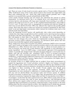
Using a large number of selected individual Hyperion channels, this supervised

classification of the four classes in the sub scene was generated; this end result is more
accurate than is normally achievable with broad band data such as obtained by Landsat:
Active microwave sensors, or radar, can use several variables to recognize crop vegetation and
even develop a classification of crop types. Here is a SIR-C (Space Shuttle) image of farmland
in the Netherlands, taken on April 4, 1994. The false colour composite was made with L-band
in the HH polarization mode = red; L-band HV = green; and C-band HH = blue.


Fig. 37. SIR-C (Space Shuttle) image of farmland in the Netherlands
An additional image variable is the crop's background, namely the nurturing soil, whose
colour and other properties can change with the particular soil type, and whose reflectance
depends on the amount of moisture it holds. Moisture tends to darken a given soil colour;
this condition is readily picked up in aircraft imagery as seen in this pair of images:


Fig. 38. Aircraft imagery showing different colours due to moisture pickup
Often, the distribution of moisture, as soil dries differentially, is variable in an imaged
barren field giving rise to a mottled or blotchy appearance. Thermal imagery brings out the

Biomass and Remote Sensing of Biomass
168
differential soil moisture content by virtue of temperature variations. The amount of water
in the crop itself also affects the sensed temperature (stressed [water deficient] or diseased
crop material is generally warmer). Soil water variations are evident in this image made by
an airborne thermal sensor of several fields, where high moisture correlates with blue and
drier parts of the fields with reds and yellows:


Fig. 39. Image made by an airborne thermal sensor of several fields showing the soil water
variations

A combination of visible, NIR, and thermal bands can pick up both water deficiency and the
resulting stress on the crops in the fields. This set of three images was made by a Daedalus
instrument flown on an aircraft. In the top image, yellow marks unplanted fields and those
in blue and green are growing crops. The center image picks up patterns of water
distribution in the crop fields. The bottom image shows levels of stress related in part to
insufficient moisture.


Fig. 40. Image showing levels of stress related in part to insufficient moisture

Introduction to Remote Sensing of Biomass
169
A passive microwave sensor also picks up soil moisture. Cooler areas appear dark in images
of fields over flown by a microwave sensor - although other factors, such as absence or
presence of growing crops (and their types) besides moisture can account for some darker
tones.
3. References
Bankert, R.L., and P.M. Tag, 1998: Using SSM/I Data and Computer Vision to Estimate
Tropical Cyclone Intensity. Proceedings, 9th Conference on Satellite Meteorology
and Oceanography, American Meteorological Society, Boston, MA, pp. 226-229.
Baum, B.A., V.Tovinkere, J.Titlow, and R.M. Welch, 1997: Automated Cloud Classification of
Global AVHRR Data Using a Fuzzy Logic Approach. Journal of Applied
Meteorology, 36, 1519-1540.
Baumgardner, M. F., Silva, L. F., Biehl, L. L. And Stoner, E. R. (1985) Reflectance properties
of soils, Advances in Agronomy, 38, 1-44.
Bojinski, S., Schaepman, M., Schaepfer, D. And Itten, K. (2003) SPECCHIO: a spectrum
database for remote sensing applications, Computers and Geosciences, 29: 27-38.
Boochs, F., Kupper, G., Dockter, K. and Kuhbauch, W. (1990) Shape of the red edge as
vitality indicator of plants, International Journal of Remote Sensing, 11 (10), 1741-1753.
Campbell, J. B. (1996) An Introduction to Remote Sensing (2nd Ed), New York, The Guilford

Press.
Clark, R. N., King, T. V. V., Ager, C. and Swayze, G. A. (1995) Initial vegetation species and
senescence/stress mapping in the San LuisValley, Colorado, using imaging
spectrometer data, Proceedings: Summitville Forum 1995,
Clark, R.N., Swayze, G.A. Gallagher, A.J., King, T.V.V. and W.M. Calvin (1993) The U. S.
Geological Survey, Digital Spectral Library, Version 1: 0.2 to 3.0 microns, U.S.
Geological Survey Open File Report 93-592, 1340 pages.
Collins, W. (1978) Remote Sensing of Crop Type and Maturity, Photogrammetric Engineering
and Remote Sensing, 44, 43-55.
Curran, P. J. (1989) Remote sensing of foliar chemistry, Remote Sensing of Environment, 30, 271-278.
Curtiss, B. and Goetz, A. F. H. (2001) Fiel Spectrometry: techniques and instrumentation,
Analytical Spectral Devices Inc,
Datt, B. (2000) Identification of green and dry vegetation components with a
crosscorrelogram spectral matching technique, International Journal of Remote
Sensing, 21, 2133-2139.
Deering, D. W. (1989) Field measurements of bidirectional reflectance: In Theory and Applications
of Optical Remote Sensing, G. Asrar (Ed.), New York, Wiley and Sons, 14-61.
Duggin, M. J. and Philipson, W. R. (1982) Field Measurement of Reflectance: some major
considerations, Applied Optics, 21 (15), 2833-2840.
Goetz, F. H. and Rowan L., C. (1981) Geologic Remote Sensing. Science, 211, 781-791
Grove, C. I., Hook, S. J. and Paylor II, E. D. (1992) Laboratory Reflectance Spectra of 160
Minerals, 0.4 to 2.5 Micrometers, Jet Propulsion Laboratory Pub, 92-2.
Hapke, B. (1993) Theory of Reflectance and Emittance Spectroscopy, UK, Cambridge University Press.
Hooker, S.B. and McClain, C.R. (2000) The calibration and validation of SeaWiFS data. Prog.
Oceanogr., 45(3-4), 427-465.
Hunt, G. R., Salisbury, J. W. and Lenhoff, C. J. (1971a) Visible and Near-Infrared spectra of
minerals and rocks: III Oxides and Hydroxides, M
odern Geology, 2, 195-205.
Hunt, G. R. (1979) Near-infrared (1.3-2.4μm) spectra of alteration minerals - Potential for use
in remote sensing, Geophysics, 44, 1974- 1986.

Biomass and Remote Sensing of Biomass
170
Irons, J.R., Weismiller, R.A. and Peterson, G.W. (1989) Soil reflectance In Theory and Applications
of Optical Remote Sensing, G. Asrar (Ed), New York, Wiley and Sons, 66–106.
King, T. V. V., Clark, R. N., Ager, C. and Swayze, G. A. (1995) Remote mineral mapping
using AVIRIS data at Summitville, Proceedings: Summitville Forum 1995, Posey, H.
H., Pendelton, J. A. and Van Zyl, D., (Eds.), Colorado Geological Survey Special
Publication 38: 59-63.
Krasnopolsky, V. M and W.H. Gemmill,, 2000, Neural network multi-parameter algorithms to retrieve
atmospheric and oceanic parameters from satellite data., Proceedings, Second Conference on
Artificial Intelligence, AMS, Long Beach, CA, 9-14 January, 2000, pp. 73-76
May, D.A., J. Sandidge, R. Holyer, and J.D. Hawkins, 1997: SSM/I Derived Tropical Cyclone
Intensities. Proceedings, 22nd Conference on Hurricanes and Tropical Meteorology,
American Meteorological Society, Boston, MA, pp. 27-28.
Milton, E. J., Rollin, E. M. and Emery, D. R. (1995) Advances in Field Spectroscopy, In
Danson, F. M. and Plummer, S. E. (1995) Advances in Environmental Remote Sensing,
UK: John Wiley and Sons.
Nicodemus, F., Richmond, J. Hsia, J., Ginsberg, I. And Limperis, T. (1977) Geometrical
Considerations and Nomenclature for Reflectance, NBS Monograph 160, US
Department of Commerce.
Pearson, Robert A. and Donald D. Bustamante, 1999. "Improving Error Structure in Temperature
Profile Retrievals from Satellite Observations", 6th International Conference on Neural
Information Processing (ICONIP'99), November 16-20, Perth, Australia.
Pfitzner, K., Bartolo, R.E., Ryan, B. and Bollhöfer, A. (2005). Issues to consider when designing a
spectral library database, Spatial Sciences Institute Conference Proceedings 2005,
Melbourne, Spatial Sciences Institute, ISBN 0- 9581366
Pfitzner, K., Bollhöfer, A. and Carr, G (2006) Protocols for measuring field reflectance
spectra. Supervising Scientist Report, In Press, Supervising Scientist for the Alligator
Rivers Region, Canberra.

Pidwirny, M. (2006). "Introduction to Geographic Information Systems". Fundamentals of
Physical Geography, 2nd Edition.
Posey, H. H., Pendelton, J. A., and Van Zyl, D., (Eds.), Colorado Geological Survey Special
Publication 38, 64-69.
Rees, W. G. (2001) Physical Principles of remote sensing, 2nd Edition, UK, Cambridge
University Press.
Rollin, E.M., Emery, D.R. and Milton, E.J. (1995) The design of field spectroradiometers, a
user’s view, In Proceedings of the 21st Annual Conference of the Remote Sensing Society,
Nottingham, UK, 555-562.
Salisbury, J. W. (1998) Spectral Measurements Field Guide, Earth Satellite Corporation, April 23
1998, Published by the Defence Technology Information Centre as Report No.
ADA362372.
Satterwhite, M. B. and Henley, J. P. (1990) Hyperspectral Signatures (400-2500 nm) of
Vegetation, Minerals, Soils, Rocks, and Cultural Features: Laboratory and Field
Measurements, U.S. Army Corps of Engineers, Engineer Topographic Laboratories,
Fort Belvoir, Virginia 22060-5546.
Schaepman, M. E. (1998) C
alibration of a Field Spectroradiometer. Calibration and Characterisation
of a non-imaging field spectroradiometer supporting imaging spectrometer validation and
hyperspectral sensor modelling, Remote Sensing Laboratories, Department of
Geography, University of Zurich, 1998.
Silva (1978) Radiation and instrumentation in remote sensing, In Swain et al., (Ed.): Remote
sensing - the quantitative approach, McGraw & Hill, 121-135.