Electric Vehicles Modelling and Simulations Part 4 ppt

Vehicle Dynamic Control of 4 In-Wheel-Motor Drived Electric Vehicle

79
According to results from Fig.2.2-6 and Fig.2.2-7, we can get that the combined control
method has better robustness to the input signal’s disturb. This point is very important to
the usage of the control method.
3. Anti-lock brake control
For electric vehicles, the motor inside each wheel is able to provide braking torque during
deceleration by working as a generator. Moreover, the torque response of an electric motor
is much faster than that of a hydraulic system. Thanks to the synergy of electric and
hydraulic brake system, the performance of the ABS (Anti-lock Brake System) on board is
considerably improved.
In this section, a new anti-skidding method based on the model following control method is
proposed. With the new feedback function and control parameter, the braking performance,
especially the phase-delay of the electric motor's torque is, according to the result of the
simulation, improved. Combined with the advantage of the origin MFC, the improved MFC
can be widely applied in anti-skidding brake control.
Furthermore, a braking torque dynamic distributor based on the adjustable hybrid braking
system is designed, so that the output torque can track the input torque accurately.
Meanwhile a sliding mode controller is constructed, which doesn’t perform with the slip
ratio value as the main control parameter. Accordingly, the total torque is regulated in order
to prevent the skidding of the wheel, so that the braking safety can be guaranteed.
3.1 Model following controller
3.1.1 One wheel model
When braking, slip ratio

is generally given by,
w
VV
V





Where V is the vehicle longitudinal velocity and Vw is the wheel velocity. Vw=Rw, where R,
w are the wheel radius and angular velocity respectively.


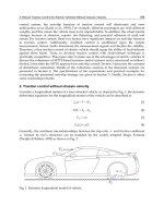
Fig. 3.1-1. One wheel model dynamic analysis

Electric Vehicles  Modelling and Simulations

80
In the light of Fig. 3.1-1, the motion equations of one wheel model can be represented as

w
I
ww
db
IdV
dw
FRT
dt R dt


(3.1-1)

M
wd
dV

F
dt


(3.1-2)
In these equations, air resistance and rotating resistance are ignored. Mw is the weight of
one wheel; I
W
is the wheel rotational inertia; T
b
is the braking torque, i.e. The sum of the
hydraulic braking torque and the braking torque offered by the electric motor, and Fd is the
braking force between the wheel and the road surface.
3.1.2 Design of MFC controller
The slip ratio is an important measurement for wheel's braking performance. For practical
vehicle, it is difficult to survey this velocity. Therefore the slip ratio is hard to obtain.
Compared with usual anti-skidding method, the method MFC(model following control) does
not depend on the information-slip ratio. Consequently it is beneficial for the practical use.
According to the result by Tokyo University:
For the situation-skidding, the transmit function is
11
()
w
skid
brake w
V
Ps
FMs


For the situation-adhesion, the transmit function is
11
()
/4
w
adh
brake w
V
Ps
FMMs



The equation above is used as the nominal model in designing the controller “Model
Following Controller”. M represents the mass of the vehicle. Applying the controller, the
dynamics of the going to be locked wheel becomes close to that of the adhesive wheel,
through which the dynamics of the vehicle will be in the emergency situation.
3.1.3 Improved MFC controller
The above listed method, especially the feedback function is based on the one-wheel-model,
but in fact there is always load-transfer for each wheel so that it cannot appropriately reflect
the vehicle’s state. According to the origin feedback function for one-wheel-model
(M/4+Mw), which is introduced in the above-mentioned text, the information of the vertical
load of each wheel can be used to substitute for (M/4+Mw). Here it is called equivalent
mass and then the controller will automatically follow the state of the vehicle, especially for
acceleration and deceleration situation.
The specific way to achieve this idea is to use each wheel’s vertical load Fz to represent its
equivalent weight. So the feedback function should be Fz/g instead of (M/4+Mw).When
necessary, there should be a wave filter to obtain a better effect.
Another aspect ,which needs mo modify is its control parameter. For the method above, the
control parameter is the wheel velocity Vw. In order to have a better improvement of the

braking performance, the wheel angular acceleration
dw
dt
as the control parameter is taken
advantage of.
Therefore the feedback function accordingly should be
2
/4*
t
R
IM R
.

Vehicle Dynamic Control of 4 In-Wheel-Motor Drived Electric Vehicle

81
With the idea of the equivalent mass, the feedback function should be
2
/*
tz
R
IF
g
R
.
The reason why we take use of this control parameter is the electric motor itself also shows a
delay (5~10ms) in an actual situation while the phase of the wheel angular acceleration
dw
dt

precedes that of the wheel velocity Vw. Consequently this control method can compensate
the phases-delay of the electric motor.
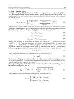
3.1.4 Simulation and results
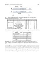
3.1.4.1 Simulation results with the wheel velocity as the control parameter
In the simulation, the peak road coefficient in the longitudinal direction is set to 0.2, which
represents the low adhesive road. The top output torque of the electric motor is 136Nm and
the delay time due to the physical characteristic of the electric motor 5 ms.
Fig. 3.1-2 shows the simulation result using the wheel velocity Vw as the control parameter.
The braking distance is apparently decreased. The slip ratio is restrained under 20%. The
unexpected increased amplitude of the slip ratio is mainly due to the delay of the electric
motor’s output, which can be proved in Fig. 3.1-2 (b). This can cause contradiction in the
braking process. Fig. 3.1-2 (c) shows longitudinal vehicle velocity and wheel velocity under
this control parameter.


(a) (b)

(c)
Fig. 3.1-2. Simulation Result of the Hybrid-ABS with the wheel velocity as the control
parameter

Electric Vehicles  Modelling and Simulations

82
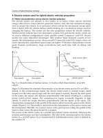
3.1.4.2 The simulation results with the angular acceleration as the control parameter
Fig. 3.1-3 shows the simulation result using the wheel angular acceleration
dw
dt
as the
control parameter and increase the top output torque of the electric motor. Compared with

the previous simulation result, it is clear that the braking distance is further shortened
(compared with the system without electric motor control). The slip ratio is also restrained
under 20% and is controlled better that the previous control algorithm. From Fig. 3.1-3 (b)
we can see the phase-delay of the electric motor is greatly improved so that the two kinds of
the torques can be simply coordinated regulated.


(a) (b)

(c)
Fig. 3.1-3. Simulation results of the Hybrid-ABS with the angular acceleration as the control
parameter
Table 2 shows the result of the braking distance and the braking time under three above-
mentioned methods.


Hydraulic ABS without
motor control
Hybrid ABS
with MFC
Hybrid ABS with
improved MFC
Braking
distance(m)
27.9 26.8 26.5
Braking time(s) 5.12 4.87 4.83
Table 2. Results of the braking distance and the braking time under three different methods

Vehicle Dynamic Control of 4 In-Wheel-Motor Drived Electric Vehicle

83
3.1.5 Conclusion
According to the simulation results, the braking performance of the improved MFC is better
than the performance of the origin MFC, proposed by Tokyo University. In future can we
modify the MFC theory through the choice of the best slip ratio, because we know the value
of the best slip ratio is not 0 but about 2.0. When we can rectify MFC theory in this aspect,
the effect of the braking process will be better.
3.2 Design of the braking torque dynamic distributor
The distributor's basic design idea is to make the hydraulic system to take over the low
frequency band of the target braking torque, and the motor to take over the high frequency
band. Then the function of the rapid adjustment can be reached.


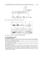
Fig. 3.2-1. The block diagram of the braking torque dynamic distributor
According to Fig. 3.2-1, C1(s) and C2(s) in Fig. 3.2-1 are the model of motor and hydraulic
system. They can be written expressed as (1) and (2):

1
1
()
1
M
Cs
s



(3.2-1)

2

1
()
1
H
Cs
s



(3.2-2)
Here,
M

and
H

are time constants for motor and hydraulic system relatively.
In order to reach the goal to track the braking torque, G
SISO
(s) =1, that is,

11 22
() () () () 1CsGs CsGs

 (3.2-3)
We can put formula (3.2-1) and formula (3.2-2) into formula (3.2-3),

111
() ()
111

motor hyd
MH
Cs Cs
sss




(3.2-4)

11
() [ () ]( 1)
11
11
()
11
motor hyd M
H
MM
hyd
H
Cs Cs s
ss
ss
Cs
ss






 




(3.2-5)

Electric Vehicles  Modelling and Simulations

84
Here, τ is the sampling step
C
hyd
(s) is chosen as the second-order Butterworth filter, and then according to (3.2-5) we can
get C
motor
(s). And the saturation torque of the motor is limited by the speed itself.
3.3 Design of the sliding mode controller
3.3.1 Design of switching function
The control target is to drive the slip ratio to the desired slip ratio. Here a switching function
is defined as:

re
f
erence
s




 (3.3-1)
The switching function is the basis to change the structure of the model. And the commonest
way to change the structure is to use sign function- sgn(s). The control law here combines
equivalent control with switching control so that the controller can have excellent
robustness in face with the uncertainty and interference of the environment.
So the control law can be expressed as:

e
q
vss
uu u

 (3.3-2)
Therefore the braking torque can be represented as:

,
s
g
n( )
bbeq
TT T s

 (3.3-3)
In practical engineering applications, the chattering may appear when sign function is used.
Therefore the Saturation function ‘sat ()’ is used to substitute for sign function.


Fig. 3.3-1. Saturation function
So the braking torque can be expressed as:

Vehicle Dynamic Control of 4 In-Wheel-Motor Drived Electric Vehicle

85

,
()
beq
b
s
TT Tsat

(3.3-4)
3.3.2 The improved sliding mode controller
One desired slip ratio can’t achieve the best braking effect because of the inaccurate
measurement of the vehicle speed and the change of the road surface. Then, a new method
based on sliding mode control will be proposed according to the characteristic of the



curve. It can seek the optimal slip ratio automatically. The typical



curve is shown in
Fig.3.3-2.


Fig. 3.3-2.



 curve
From Fig. 3.3-2, we can see:
When
d
0
d



,
re
f
erence


 ,

needs increasing in order to obtain larger

. At this point we
can increase the braking torque on the wheel;
When
d
0
d



,
re

f
erence



,

needs maintaining in order to obtain larger

. At this point
we can maintain the braking torque on the wheel;
When
d
0
d



,
re
f
erence


 ,

needs decreasing in order to obtain larger

. At this point we
can decrease the braking torque on the wheel.

According to the one wheel model and the definition of slip ratio, we can receive:

/
/
bw x
Z
bw x
Z
TIwV
dddt
dddt FR
Rw
TIwV
FR
w







 

 
(3.3-5)

Electric Vehicles  Modelling and Simulations

86

That is:

When 0
bw
TIw
w




,

<
re
f
erence

,
re
f
erence
s



 <0

When 0
bw
TIw

w




,

=
re
f
erence

,
re
f
erence
s



 =0

When 0
bw
TIw
w





,

>
re
f
erence

,
re
f
erence
s




>0

The interval of the optimal slip ratio is commonly from 0.1 to 0.2. Therefore, when the slip
ratio calculated by
x
x
RV
V



 is larger than 0.3, we can judge that the current slip ratio is
surely larger than the optimal slip ratio. The output of the sign function is 1.
So the algorithm based on




curve can be improved as:
When the slip ratio calculated by
x
x
RV
V



 is bigger than 0.3, then we know that the
actual slip ratio must be bigger than the optimal slip ratio, then the output of the sign
function is 1;
When the slip ratio calculated by
x
x
RV
V



 is smaller than 0.3,
i.
If ||
w
w




，

0
s
g
n( ) 1
s
g
n( ) 1
0
wb
w
wb
w
JT
s
JT
s































ii. If||
w
w




Sign function maintains the output of the last step, that is:
1
s
g

n( ) s
g
n( )
tt
ss


.
3.3.3 Simulation and results
Fig. 3.3-3 shows the effect of the braking torque dynamic distributor. Since the existence of
the saturation torque of the motor, it can’t track the input torque when the input torque too
large. When the demand torque is not too large, the braking torque dynamic distributor
illustrates excellent capability.

Vehicle Dynamic Control of 4 In-Wheel-Motor Drived Electric Vehicle

87

Fig. 3.3-3. The character of the braking torque dynamic distributor

Electric Vehicles  Modelling and Simulations

88
Fig.3.3-4 - Fig.3.3-6 is the simulation results, which get from the improved sliding mode
controller, and the initial velocity of the vehicle is 80km/h, the saturation torque of the
motor is 180Nm
：
i.
When adhesion coefficient


0.9:

Fig. 3.3-4. Simulation results on the road with


0.9

Vehicle Dynamic Control of 4 In-Wheel-Motor Drived Electric Vehicle

89
ii. When adhesion coefficient


0.2:






Fig. 3.3-5. Simulation results on the road with µ = 0.2

Electric Vehicles  Modelling and Simulations

90
iii. When adhesion coefficient changes in 1
st
second from 0.2 to 0.9:

Fig. 3.3-6. The road adhesion coefficient changes from


0.2 to


0.9 at the 1
st
second

Vehicle Dynamic Control of 4 In-Wheel-Motor Drived Electric Vehicle

91
From Fig.3.3-4 -Fig.3.3-6, we know that, although this method doesn’t regard slip rate as the
main control information, this sliding mode can track the optimal slip ratio automatically.
That means, both the longitudinal adhesion force and the lateral adhesion force can be made
use of fully. Even on the road, whose adhesion coefficient increases suddenly, the controller
can also find the optimal slip ratio.
During the braking process, the torque offered by the motor and hydraulic system doesn’t
oscillate distinctly. It indicates, the hybrid-braking system can achieve target braking torque
actually.
Table 3 shows the braking distance and braking time on the different road. From the datum
we know the braking safety can be guaranteed with this anti-skidding controller.

Number Adhesion coefficient Braking distance(m) Braking time(s)

a) 0.9 33.99 2.71
b) 0.2 136.6 11.62
c) 0.2-0.9 50.23 3.47
Table 3. Braking distance and braking time on the different road
3.3.4 Conclusion
The braking torque dynamic distributor, which combines the merits of the two actuators
motor and hydraulic system, can track the demanded torque promptly and effectively. The
sliding mode controller has two sorts. One is to track the desired slip ratio, which is set
manually and the effect of the controller good. However, the measurement of the vehicle
velocity and the identification of the road limit the promotion of the usage. The other kind
of controller can seek the optimal slip ratio automatically. Through the result of the
simulation, the effectiveness of this controller is proved. It can have a wider range of
application.
4. Vehicle stability control
Many researchers in the last decade have reported that direct yaw moment control is one of
the most effective methods of active chassis control, which could considerably enhance the
vehicle stability and controllability. The direct yaw moment control of a traditional ICE
(Internal Combustion Engine) vehicle is based on the individual control of wheel braking
force known as the differential braking. However, for EVs, the generation of desired yaw
moment for stabilizing the vehicle under critical driving conditions can be achieved by rapid
and precise traction/braking force control of each in-wheel-motor.
In this section, a hierarchical vehicle stability control strategy is introduced.
The high level of the control strategy is the vehicle motion control level. A dynamic control
system of a 4 in-wheel-motored electric vehicle which improves the controlling stability
under critical situation is presented. By providing the method of estimating the cornering
stiffness and combining the controller with optimal control allocation algorithm, which
takes account of the couple characteristic of the longitudinal/lateral force for tire under
critical situation, the vehicle stability control system is designed. The double lane change
simulation was carried out to verify the validity of the control method. Simulation result
shows the proposed control method could stabilize the vehicle posture well under critical

condition. Compared with the LQR with fixed cornering stiffness, the feedback from

Electric Vehicles  Modelling and Simulations

92
identifying cornering stiffness to correct the parameters of the controller helps a lot in
improving the robustness of the stability control.
The low level of the control strategy is the control allocation level, in which the longitudinal
force’s distribution is the focal point. Through the analysis of the tire characteristics under
the combined longitudinal and lateral forces, an effectiveness matrix for the control
allocation considering the longitudinal force’s impact on the lateral force was proposed.
Based on Quadratic Programming method the longitudinal forces on each wheel are optimal
distributed. The simulation results indicate that the proposed method can enhance the
vehicle handling stability, meanwhile the control efficiency is improved as well.
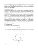
4.1 Vehicle dynamic control structure
Studies have shown that hierarchical control of the dynamics control method has a clear,
modular control structure, as well as better control robustness, which is easy for real vehicle
applications of the control algorithms. This hierarchical control architecture is widely
adopted by general chassis’s integrated control.VDC(vehicle dynamic control) introduces
the hierarchical control structure, as shown in Fig. 4.1-1, the upper level is the vehicle
motion control and the bottom level is the control allocation for each actuator.
The motion controller which belongs to the first level in the stability algorithm, collects the
signals from the steering wheel’s angle and the accelerator pedal, and calculates the
generalized forces required by the stability control, including the longitudinal forces
xT
F

and yaw moment
zT
M

. The longitudinal forces can be directly calculated according to the
accelerator pedal signals. The yaw moment can be got by following the reference model.


Fig. 4.1-1. Vehicle dynamic control structure
The control allocation is the second level of the vehicle controller. It is responsible to convert
the "generalized forces" to the sub-forces on each actuator according to certain distribution
rules and under some external constraint conditions (such as the maximum output of the
motor and the road adhesion coefficient, etc.). And then to realize the optimum distribution
of the each motor’s torque. For a 4WD electric vehicle driven by 4 in-wheel-motors, the sub-
force on each actuator is just the tire longitudinal force formed by the motor’s output torque.

Vehicle Dynamic Control of 4 In-Wheel-Motor Drived Electric Vehicle

93
4.2 Vehicle motion controller
The yaw moment control is based on the MFC (model follow control) method. As reference
model, the DYC model could keep slip angle zero for stability. The gain scheduling control
algorithm can revise the parameters real-timely through the cornering stiffness
identification to improve the adaptability of the algorithm to the environment and the
change of the model parameters. The variable structure control (VSC) is applied to design
control algorithm, for considering the strong robust characteristic during uncertainty. With
proposed non-linear vehicle model, a precise gain value for switch function will be
calculated, in order to reduce chattering effect.
4.2.1 Vehicle model
4.2.1.1 Linear vehicle model
The simplified linear two freedom model make the side slip angle and the yaw rate as its
state variables. As the control input, the yaw moment
zT
M

is gained from the longitudinal
force allocation by the motors according to the required moment, the function is:


()
yf y
r
d
mV F F
dt



(4.2-1)


z
y
zT
d
JMM
dt


(4.2-2)

The description of the state space is:


XAXE Bu




(4.2-3)

Here： []
T
x


 ,
zT
uM

2
22
2( ) 2( )
1
2( ) 2( )
fr ffrr
ff rr ff rr
zz
CC ClCl
mV
mV
A
Cl Cl Cl Cl
JJV






















2
0
,
1
2
f
ff
z
z
C
mV

EB
Cl
J
J

















(4.2-4)
yyffy
rr
M
Fl Fl represents the yaw motion caused by the lateral force acting on each wheel,
yf
F ，
y
r

F are the total front/rear wheel lateral forces. Other parameters are shown in
Fig.4.2-1.

Electric Vehicles  Modelling and Simulations

94

Fig. 4.2-1. Planar vehicle motion model
4.2.1.2 Non-linear vehicle model
In this paper the arc-tangent function is used to fit the lateral force formula, then a simple
non-linear vehicle model can be obtained, the arc-tangent function contains two fitting
parameters
12
,cc, the fitting effect is show below:
The state space of One-track non-linear vehicle model can be express
as:
12 () 1
[][],
TT
x
xx h x
 
  x

,

is the centroid-side angle of the vehicle,

is the
course angle of the vehicle,

u means additional yaw moment input
zT
M
, the complete
function is:

0 0.1 0.2 0.3 0.4 0.5 0.6
0
1000
2000
3000
4000
5000
6000
7000
slip angle /rad
tire lateral force/N


Magic model
arc tangent function
c1*atan(c2*alfa)

Fig. 4.2-2. Arc-tangent function vs. magic model

Vehicle Dynamic Control of 4 In-Wheel-Motor Drived Electric Vehicle

95

1212

12122
1
2
1212
1212
1
{atan[( )]cos
atan[ ( )]}
1
{atan[( )]cos
atan[ ( )] }
f
fff f
r
rr
f
ff f f f
z
r
rr r
l
ccxx
mv V
l
ccxxx
x
V
l
x
lc c x x

JV
l
lc c x x u
V




























(4.2-5)
Here, m represents the mass of the vehicle,
z
J represents the yaw rotational inertia of the
vehicle,
1
f
c and
2
f
c are the fitting parameters for the front wheel,
1r
c and
2r
c are the fitting
parameters for the rear wheel,
f
l is the distance from the gravity point to the front axle and
r
l is the distance from the gravity point to the rear axle, V is the gravity point velocity of the
vehicle,
f

is the steering angle for the front wheel.
Based on non-linear model mention above, we can design yaw-rate follow controller. In our
case, the dynamic function of yaw rate is second-order system:

(,) (,) () ()
1

((,,) (,,))
1
(,) ()
yf f f
z
fy
rrrz r
z
z
fXt fXt gu dt
FFlFFl
J
fXt u dt
J

 

  

 
  

(4.2-6)
Here,
f

is the side slip angle for the front wheel,
r

is the side slip angle for the rear

wheel,
yf
F and
y
r
F are the side slip force for the front and rear wheel,
f
z
F and
rz
F
are the
vertical load for the front and rear wheel,

is the road adhesion coefficient.
(,)fXt
indicates non-linear system function;
()gu
indicates non-linear continued function;
(,)fXt
and
()dt
stand for uncertainty and external disturbance of controlled object, which
are supposed to be zeros.
4.2.2 Reference model
The desired yaw-rate output is calculated from the reference model (DYC):

1
d
dd

dd
k



  

(4.2-7)
Here:
2
2
2( )
f
d
ff
rr
CV
k
mV C l C l


；
22
2( )
z
d
ff rr
JV
Cl Cl






4.2.3 Controller design
4.2.3.1 Gain scheduling controller
Based on the linear vehicle model, the controller adapts the LQR stability control algorithm.
It is composed of feed-forward and feedback. Supposing the relationship between the feed-
forward yaw moment and the front-wheel steering angle as:

Electric Vehicles  Modelling and Simulations

96
() ()
ff ff
M
sG s


(4.2-8)
Here:
ff
G is the feed-forward yaw moment coefficient. It can be calculated through the
transfer function from vehicle side slip angle to front-wheel steering angle under stable
condition, i.e.
() ()ss


when (0) 0



. Then.

2
2
42
2( )
frfr ff
ff
ff rr
CCll ClmV
G
mV C l C l



(4.2-9)
Feedback control is used to decrease the control system’s error caused by the unknown
perturbation and the imprecise of the model, and to improve the reliability of the control
system.
Define the state error
d
EXX
, from function (4.2-3), (4.2-7):
()()
fb d d d
EAEBM AAX EE

  


(4.2-10)
Considering the last two as perturbation, and according to LQR, assure the target function
below to be least:

0
()
TT
JEQEuRudt



(4.2-11)
By solving the Riccati function
， feedback coefficient
f
b
G is gained. And the feedback
moment is:

12
()()
f
b
f
b
f
bd
f
bd
MGEg g




  

(4.2-12)
Total yaw moment required is:

zT
ff f
b
M
MM

 (4.2-13)
From the analysis above, we know the total yaw moment is decided by the feed-forward
coefficient
ff
G and feed-back coefficient
f
b
G together. And the coefficients can be adjusted
on time according to the front and rear cornering stiffness identified and the vehicle speed
measured. The control algorithm refers to the linear optimization calculation and on-line
resolution of the Riccati function, which can affect the real time performance. On the real car
the coefficients corresponding to different cornering stiffness and the vehicle speed are
calculated off-line previously. Then a look-up table will be made from that and will be
downloaded to the ECU for control. To easily show the movement of the feed-forward and
feed-back coefficients, the following figure will illustrate the change of the front and rear
cornering stiffness together through supposing the front cornering stiffness is changing,

while the rear one is a fixed proportion to it.
Cornering stiffness is an important parameter for the controller. It will change along with
the road condition or under the critical condition of the vehicle, which will further affect the
control precise of the vehicle stability. The cornering stiffness that DYC control relies on is
linear to the cornering stiffness under the current condition. So the cornering stiffness in this
paper is estimated based on the two freedom linear model.

Vehicle Dynamic Control of 4 In-Wheel-Motor Drived Electric Vehicle

97
0
5
10
15
x 10
4
0
10
20
30
40
-2
0
2
4
6
8
x 10
6
front tire cornering

stiffness[N/rad]
vehicle velocity[m/s]
feed-forward gain


0
5
10
15
x 10
4
0
20
40
0
1
2
3
4
x 10
4
vehicle velocity[m/s]
front tire cornering stiffness[N/rad]
yaw rate feedback gain


0
5
10
15

x 10
4
0
10
20
30
40
-800
-600
-400
-200
0
vehicle velocity[m/s]
front tire cornering
stiffness[N/rad]
beta feedback gain

Fig. 4.2-3. Feed-forward/Feed-back Map

Electric Vehicles  Modelling and Simulations

98
From function (4.2-2) ,
y
M
is:

2( ) 2( )
f
r

yf fr r
l
l
M
ClCl
VV
 
 (4.2-14)
Here ,
f
r
CCare front and rear nominal cornering stiffness.
y
M
above needs to be estimated
by the yaw moment observation(YMO) below:


ˆ
()( )
y
zzT
MFsJ M



(4.2-15)

Here: () /( )
cc

Fs s


is a filter function to gain


.
c

is truncation frequency.
From function (4.2-14): to estimate the front and rear cornering stiffness separately, the
estimator must provide the information of

. Therefore a united estimation of , ,
fr
CC


needs to be established. To simplify the design, some change has been made to the function
above. According to the magic tire model, the wheel cornering stiffness is pro rata to the
load under a certain load range ( )
ff
rr
Cl Cl

. And as

is a small value, then:

ff
rr
y
Cl Cl M



 ； (4.2-16)
Thus function (4.2-14) can be
：

2( )
fr
yff
ll
MCl
V




 (4.2-17)

ˆ
() (), ,
TT
yf
M
ttC
 

  (4.2-18)

() () 2 ( )
fr
f
ll
tFs l
V




 



(4.2-19)
Based on the above model, the front and rear cornering stiffness
,
f
r
CC
will be gained by
RLS estimation, as follows:



 







(1)()
ˆˆ
() ( 1)
()( 1)()
ˆ
()( 1) ()
T
T
kk
kk
kk k
kk yk


(1)
1
()
(1)()()(1)
()( 1)()
T
T
k
k
kkkk
kk k



 






 






(4.2-20)

is forget factor and can be properly selected according to the road condition.
With the estimation result the controller parameters can be corrected on time. And a more
precise general force can be gained to improve the allocation control of the vehicle.

Vehicle Dynamic Control of 4 In-Wheel-Motor Drived Electric Vehicle

99
4.3 Control alloction alogrithm
Through the control of the upper level, the yaw moment
zT
M
is gained, which will be
allocated to each actuator to realize the control target (on 4WD EV is the motor torque).

4.3.1 Effectiveness matrix
Making approximation: sin 0


and cos 1


, the total vehicle longitudinal force and the
yaw moment caused by the longitudinal force are as follows:

()
2
xT xfl xfr xrl xrr
zxT x
f
lx
f
rxrlxrr
FFFFF
b
MFFFF

  
(4.3-1)
Expressed as:

xT x x
zT zx x
FB
MB



(4.3-2)
Where: [ ]
T
xx
f
lx
f
rxrlxrr
FFFF ; [1111]
x
B

,
[]
22 22
zx
bb bb
B  
,
x
B and
zx
B
are named as the effectiveness matrix.
In most researches, the vehicle yaw moment was directly obtained by (4.3-1). As the
coupling characteristics of tires, the change of the tire longitudinal forces leads to the change
of its’ lateral force, especially in the critical conditions. So it’s necessary to consider the
additional yaw moment caused by the change of the lateral force.

Under certain tire sideslip angle

, the relationship between the four wheels’ lateral and
longitudinal forces can be expressed as:
()
yy
xx
f

 (4.3-3)
Where: [ ]
T
y yfl yfr yrl yrr
FFFF
y
x
f

is a non-linear function, which brings complexity in the computation of the effectiveness
matrix and the optimization of the control distribution. While if direct linear approximation
was made to it, it would be too simplistic.
Discretization of the total yaw moment demand from the vehicle motion controller comes
to:





1
zT zT zT

Mt Mt M 
(4.3-4)
Supposing that

is a small value, then sin 0

 and cos 1


. The increment of the total
yaw moment can be expressed as:

BB
zT zx x z
yy
M

FF
(4.3-5)
Here:
22 22
zx
bb bb
B

 


，
z

yff
rr
Bllll








Electric Vehicles  Modelling and Simulations

100
T
x xfl xfr xrl xrr
FFFF


   


F

T
y yfl yfr yrl yrr
FFFF


   



F

Under a certain tire cornering angle

, the coupling relation of the tire longitudinal/lateral
forces can be expressed as:



yy
xx
f

FF (4.3-6)
Here:
T
x xfl xfr xrl xrr
FFFF



F ,
T
y yfl yfr yrl yrr
FFFF






F .
then:


yy
xx
f

 FF
Magic formula can describe the tire characteristics under the combined working condition,
but too complex. According to tire friction ellipse, the tire characteristics can be
approximated expressed as:
2
2
0max
1
y
x
yx
F
F
FF












, where
0
y
F

is lateral tire force under tire
sideslip angle

when longitudinal force equal zero, and
maxx
F

is maximum longitudinal tire
force under tire sideslip angle

.


i j
i j
2
0
2
max
0

i
yi xi
yx
yi x i
ij
FF
f
FF















(4.3-7)
To substitute function (4.3-5) with (4.3-7), then:

()
zzxz
yy
xx

M
BBfF



(4.3-8)
Then:
Set virtual control vector

T
xT zT
vF M  ,
where the total longitudinal forces
xT
F are created by the driver’s pedal command. And the
actual control vector [ ]
T
x
f
lx
f
rxrlxrr
uF F F F    . Then the control allocation should
meet the following equation:
vBu

 (4.3-9)
Where: the effectiveness matrix
x
zx z

yy
x
B
B
BBf












4.3.2 Optimal allocation algorithm
One objective of the control allocation can be expressed as to minimize the allocation error:

Vehicle Dynamic Control of 4 In-Wheel-Motor Drived Electric Vehicle

101

min ( )

v
WBuv
st u u u




(4.3-10)
v
W is the weight matrix, reflecting the priority of each generalized force. The constraints
include the limited capacity of the actuator, ie. the maximum torque range of in-wheel-
motors, and the road adhesion ability.
At the same time, we also hope to minimize the energy consumption of the actuator.
Considering the characteristics of the tire adhesion, different wheels with different vertical
load
z
F
, then the longitudinal forces and the lateral forces provided by each wheel are not
the same. So the weight matrix
u
W is introduced. It is a diagonal matrix, and the diagonal
elements are:

222
1
()( )
ii
ii zii xii
y
ii
w
FFF




(4.3-11)
Where

is the road adhesion coefficient of each wheel.
x
F ,
y
F and
z
F are the longitudinal
force, the lateral force and the vertical load of each wheel of the time.
Then another objective can be expressed as:

min ( )

ud
Wuu
st u u u




(4.3-12)
u
W considerate the characteristic of each tire adhesion, because different wheel is with
different vertical load
z
F .
The above (4.3-10) and (4.3-12) can be combined as followed Quadratic Programming (QP)
problem:

22
22
arg min ( ( ) ( ) )
ud
uuu
uWuuWBu





(4.3-13)
Thus the computation time can be reduced largely. The parameter  is usually set to very
large in order to minimize the allocation error. The optimization problem can be solved
through active set methods.
4.4 Simulation results and analysis
Using vehicle dynamics analysis software veDYNA, combined with the proposed vehicle
stability control algorithm above, the high velocity double lane change operation is
simulated to verify the validity of the control algorithm.
The vehicle is to carry out double lane change operation with the velocity of about 100km/h,
which should be as constant as possible during the operation. Fig.4.4-2 shows the contrast
between the vehicle trajectories with and without stability control. The vehicle could keep a
steady posture and avoid obviously lateral slippage. Meanwhile compared to the LQR control
without identification of the cornering stiffness, the algorithm designed in this paper can
decrease the impact of the change of the model’s parameters on the control effect. In addition a
little under steering during lane change presents the steering characteristic of DYC reference
model to restrain over large side slip angle.

Electric Vehicles  Modelling and Simulations

102




Fig. 4.4-1. veDYNA Simulation Model



0 20 40 60 80 100
-2
-1
0
1
2
3
4
5
x-position [m]
y-position [m]
Double lane change


without control
LQR control
with estimation LQR control

Fig. 4.4-2. Vehicle Trajectory

Vehicle Dynamic Control of 4 In-Wheel-Motor Drived Electric Vehicle

103
8 10 12 14 16 18
-1
-0.5
0
0.5
1
time(s)
yaw -rate(rad/s)


actual yawrate
desired yawrate
-0.2 -0.1 0 0.1 0.2
-0.4
-0.2
0
0.2
0.4
0.6
slip-angle(rad)
gradient of slip-angle(rad/s)

0 1 2 3 4 5
-10
-5
0
5

10
Time [s]
Lateral acceleration [m/s
2
]
0 1 2 3 4 5
-4
-2
0
2
4
6
Time [s]
Roll angle [deg]

Fig. 4.4-3. Vehicle States
Fig. 4.4-3 presents the behaviors of several state values of the vehicle during such operation.
Among them the yaw rate response can match the desired value well. Supposing on level
and smooth road, when the peak value of the lateral acceleration is close to 1.0g, the vehicle
has been working under critical condition. The




phase trajectory indicates that the
vehicle can keep steady even when the slip angle reaches 8 degree.

5 10 15 20
0
0.5

1
1.5
2
2.5
3
x 10
4
time[s]
cornering stiffness[N/rad]


front tire estimated value
rear tire estimated value

Fig. 4.4-4. Estimated Cornering Stiffness of Tire