Electric Vehicles Modelling and Simulations Part 1 pdf
Bạn đang xem bản rút gọn của tài liệu. Xem và tải ngay bản đầy đủ của tài liệu tại đây (798.18 KB, 30 trang )
ELECTRICVEHICLES–
MODELLINGAND
SIMULATIONS
EditedbySerefSoylu
Electric Vehicles – Modelling and Simulations
Edited by Seref Soylu
Published by InTech
Janeza Trdine 9, 51000 Rijeka, Croatia
Copyright © 2011 InTech
All chapters are Open Access articles distributed under the Creative Commons
Non Commercial Share Alike Attribution 3.0 license, which permits to copy,
distribute, transmit, and adapt the work in any medium, so long as the original
work is properly cited. After this work has been published by InTech, authors
have the right to republish it, in whole or part, in any publication of which they
are the author, and to make other personal use of the work. Any republication,
referencing or personal use of the work must explicitly identify the original source.
Statements and opinions expressed in the chapters are these of the individual contributors
and not necessarily those of the editors or publisher. No responsibility is accepted
for the accuracy of information contained in the published articles. The publisher
assumes no responsibility for any damage or injury to persons or property arising out
of the use of any materials, instructions, methods or ideas contained in the book.
Publishing Process Manager Ivana Lorkovic
Technical Editor Teodora Smiljanic
Cover Designer Jan Hyrat
Image Copyright AlexRoz, 2010. Used under license from Shutterstock.com
First published August, 2011
Printed in Croatia
A free online edition of this book is available at www.intechopen.com
Additional hard copies can be obtained from
Electric Vehicles – Modelling and Simulations, Edited by Seref Soylu
p. cm.
978-953-307-477-1
free online editions of InTech
Books and Journals can be found at
www.intechopen.com
Contents
Preface IX
Chapter 1 Electrical Vehicle Design and Modeling 1
Erik Schaltz
Chapter 2 Modeling and Simulation of High
Performance Electrical Vehicle Powertrains in VHDL-AMS 25
K. Jaber, A. Fakhfakh and R. Neji
Chapter 3 Control of Hybrid Electrical Vehicles 41
Gheorghe Livinţ, Vasile Horga,
Marcel Răţoi and Mihai Albu
Chapter 4 Vehicle Dynamic Control of 4
In-Wheel-Motor Drived Electric Vehicle 67
Lu Xiong and Zhuoping Yu
Chapter 5 A Robust Traction Control for
Electric Vehicles Without Chassis Velocity 107
Jia-Sheng Hu, Dejun Yin and Feng-Rung Hu
Chapter 6 Vehicle Stability Enhancement Control for
Electric Vehicle Using Behaviour Model Control 127
Kada Hartani and Yahia Miloud
Chapter 7 FPGA Based Powertrain Control for Electric Vehicles 159
Ricardo de Castro, Rui Esteves Araújo and
Diamantino Freitas
Chapter 8 Global Design and Optimization of a Permanent Magnet
Synchronous Machine Used for Light Electric Vehicle 177
Daniel Fodorean
Chapter 9 Efficient Sensorless PMSM Drive
for Electric Vehicle Traction Systems 199
Driss Yousfi, Abdelhadi Elbacha and Abdellah Ait Ouahman
VI Contents
Chapter 10 Hybrid Switched Reluctance
Motor and Drives Applied on a Hybrid Electric Car 215
Qianfan Zhang, Xiaofei Liu, Shumei Cui, Shuai Dong and Yifan Yu
Chapter 11 Mathematical Modelling and Simulation of a PWM Inverter
Controlled Brushless Motor Drive System from Physical
Principles for Electric Vehicle Propulsion Applications 233
Richard A. Guinee
Chapter 12 Multiobjective Optimal Design
of an Inverter Fed Axial Flux Permanent
Magnet In-Wheel Motor for Electric Vehicles 287
Christophe Versèle, Olivier Deblecker and Jacques Lobry
Chapter 13 DC/DC Converters for Electric Vehicles 309
Monzer Al Sakka, Joeri Van Mierlo and Hamid Gualous
Chapter 14 A Comparative Thermal Study of Two Permanent Magnets
Motors Structures with Interior and Exterior Rotor 333
Naourez Ben Hadj, Jalila Kaouthar Kammoun,
Mohamed Amine Fakhfakh, Mohamed Chaieb and Rafik Neji
Chapter 15 Minimization of the Copper Losses in Electrical Vehicle
Using Doubly Fed Induction Motor Vector Controlled 347
Saïd Drid
Chapter 16 Predictive Intelligent Battery Management
System to Enhance the Performance of Electric Vehicle 365
Mohamad Abdul-Hak, Nizar Al-Holou and Utayba Mohammad
Chapter 17 Design and Analysis of Multi-Node
CAN Bus for Diesel Hybrid Electric Vehicle 385
XiaoJian Mao, Jun hua Song,
Junxi Wang, Hang bo Tang and Zhuo bin
Chapter 18 Sugeno Inference Perturbation
Analysis for Electric Aerial Vehicles 397
John T. Economou and Kevin Knowles
Chapter 19 Extended Simulation of an Embedded Brushless
Motor Drive (BLMD) System for Adjustable Speed
Control Inclusive of a Novel Impedance Angle
Compensation Technique for Improved Torque
Control in Electric Vehicle Propulsion Systems 417
Richard A. Guinee
Preface
Electric vehicles are becoming promising alternatives to be remedy for urban air
pollution, green house gases and depletion of the finite fossil fuel resources (the
challenging triad) as they use centrally generated electricity as a power source. It is
well known that power generation at centralized pl ants are much more
efficient and
their emissions can be controlled much easier than those emitted from internal
combustionengines thatscatteredallovertheworld.Additionally,anelectricvehicle
can convert the vehicle’s kinetic energy to electrical energy and store it during the
brakingandcoasting.
Allthebenefitsofelectricalvehiclesarestarting
tojustify,acenturylater,attentionof
industry, academia and policy makers again as promising alternatives for urban
transport.Nowadays,industryandacademiaarestrivingtoovercome thechallenging
barriersthatblockwidespreaduseofelectricvehicles.Lifetime,energydensity,power
density, weight and cost of battery packs are major
barriers to overcome. However,
modeling and optimization of other components of electric vehicles are also as
important as theyhave strong impacts on theefficiency, drivability and safety of the
vehicles.Inthissensethereisgrowingdemandforknowledgetomodelandoptimize
theelectricalvehicles.
In this book, modeli ng
and simulation of electric vehicl es and their components
have been emphasized chapter by chapter with valuable contribution of many
researchers who work on both technical and regulatory sides of the field.
Mathematical models for electrical vehicles and their components were introduced
and merged together to make this book a guide
for industry, academia and policy
makers.
To be effective chapters of the book were de signed in a logical order.It started with
the examination ofdynamicmodels andsimulation results for electricalvehicles and
tractionsystems.Then, modelsforalternativeelectricmotorsanddrivesystemswere
presented. After that, models for
power electronic components and various control
systems were examined. Finally, to establish the required knowledge as a whole, an
intelligentenergymanagementsystemwasintroduced.
X Preface
Astheeditorofthisbook,Iwouldliketoexpressmygratitudetothechapterauthors
for submitting such valuable works that were already published or presented in
prestigious journals andconferences. I hopeyou will getmaximum benefitfromthis
booktotaketheurbantransportsystemtoa
sustainablelevel.
SerefSoylu,PhD
SakaryaUniversity,DepartmentofEnvironmentalEngineering,Sakarya,
Turkey
0
Electrical Vehicle Design and Modeling
Erik Schaltz
Aalborg University
Denmark
1. Introduction
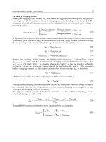
Electric vehicles are by many seen as the cars of the future as they are high efficient, produces
no local pollution, are silent, and can be used for power regulation by the grid operator.
However, electric vehicles still have critical issues which need to be solved. The three main
challenges are limited driving range, long charging time, and high cost. The three main
challenges are all related to the battery package of the car. The battery package should both
contain enough energy in order to have a certain driving range and it should also have a
sufficient power capability for the accelerations and decelerations. In order to be able to
estimate the energy consumption of an electric vehicles it is very important to have a proper
model of the vehicle (Gao et al., 2007; Mapelli et al., 2010; Schaltz, 2010). The model of an
electric vehicle is very complex as it contains many different components, e.g., transmission,
electric machine, power electronics, and battery. Each component needs to be modeled
properly in order prevent wrong conclusions. The design or rating of each component is a
difficult task as the parameters of one component affect the power level of another one. There
is therefore a risk that one component is rated inappropriate which might make the vehicle
unnecessary expensive or inefficient. In this chapter a method for designing the power system
of an electric vehicle is presented. The method insures that the requirements due to driving
distance and acceleration is fulfilled.
The focus in this chapter will be on the modeling and design of the power system of a battery
electric vehicle. Less attention will therefore be put on the selection of each component
(electric machines, power electronics, batteries, etc.) of the power system as this is a very big
task in it self. This chapter will therefore concentrate on the methodology of the modeling and
design process. However, the method presented here is also suitable for other architectures
and choice of components.
The chapter is organized as follows: After the introduction Section 2 describes the modeling
of the electric vehicle, Section 3 presents the proposed design method, Section 4 provides a
case study in order to demonstrate the proposed method, and Section 5 gives the conclusion
remarks.
2. Vehicle modeling
2.1 Architecture
Many different architectures of an electric vehicle exist (Chan et al., 2010) as there are many
possibilities, e.g., 1 to 4 electric machines, DC or AC machines, gearbox/no gearbox, high or
1
2 Will-be-set-by-IN-TECH
low battery voltage, one or three phase charging, etc. However, in this chapter the architecture
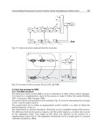
in Fig. 1 is chosen.
The purpose of the different components in Fig. 1 will here shortly be explained: The traction
power of the wheels is delivered by the three phase electric machine. The torque of the left
and right wheels are provided by a differential with also has a gear ratio in order to fit the high
speed of the electric machine shaft to the lower speed of the wheels. The torque and speed
of the machine are controlled by the inverter which inverts the battery DC voltage to a three
phase AC voltage suitable for the electric machine. When analyzing the energy consumption
of an electric vehicle it is important also to include the losses due to the components which
not are a part of the power chain from the grid to the wheels. These losses are denoted as
auxiliary loss and includes the lighting system, comfort system, safety systems, etc. During
the regenerative braking it is important that the maximum voltage of the battery is not
exceeded. For this reason a braking resistor is introduced. The rectifier rectifies the three
phase voltages and currents of the grid to DC levels and the boost converter makes it possible
to transfer power from the low voltage side of the rectifier to the high voltage side of the
battery.
(OHFWULF
PDFKLQH
7UDQVPLVVLRQ
,QYHUWHU
Z
Z
Z
Z
V
V
L
$
L
%
L
&
L
,QY
L
%DW
$X[L
OLDU\
ORDGV
L
$X[
%RRVW
FRQ
YHUWHU
L
%&
L
5)
5HFWLILHU
Y
5)
*ULG
L
8
L
9
L
:
Y
9
Y
8
Y
:
%UDNLQJ
UHVLVWRU
L
%5
%DWWHU\
Y
%DW
Fig. 1. Architecture of the battery electric vehicle. In the figure the main components of the
vehicles which have an influence on the energy consumption of the vehicle is shown.
2.2 Force Model
The forces which the electric machine of the vehicle must overcome are the forces due to
gravity, wind, rolling resistance, and inertial effect. These forces can also be seen in Fig. 2
where the forces acting on the vehicle are shown.
f
wind
f
t
f
rr
f
I
v
car
f
g
f
n
α
Fig. 2. Free body diagram of the forces (thick arrows) acting on the car.
2
Electric Vehicles – Modelling and Simulations
Electrical Vehicle Design and Modeling 3
The traction force of a vehicle can be described by the following two equations (Ehsani et al.,
2005):
f
t
= M
car
˙
v
car
f
I
+ M
car
· g
f
g
·sin(α)+sign(v
car
)
f
n
M
car
· g ·cos(α) ·c
rr
f
rr
+ sign(v
car
+ v
wind
)
1
2
ρ
air
C
drag
A
front
(
v
car
+ v
wind
)
2
f
wind
(1)
c
rr
= 0.01
1 +
3.6
100
v
car
,(2)
where f
t
[
N
]
Traction force of the vehicle
f
I
[
N
]
Inertial force of the vehicle
f
rr
[
N
]
Rolling resistance force of the wheels
f
g
[
N
]
Gravitational force of the vehicle
f
n
[
N
]
Normal force of the vehicle
f
wind
[
N
]
Force due to wind resistance
α
[
rad
]
Angle of the driving surface
M
car
[
kg
]
Mass of the vehicle
v
car
[
m/s
]
Velocity of the vehicle
˙
v
car
m/s
2
Acceleration of the vehicle
g
= 9.81
m/s
2
Free fall acceleration
ρ
air
= 1.2041
kg/m
3
Air density of dry air at 20
◦
C
c
rr
[
−
]
Tire rolling resistance coefficient
C
drag
[
−
]
Aerodynamic drag coefficient
A
front
m
2
Front area
v
wind
[
m/s
]
Headwind speed
2.3 Auxiliary loads
The main purpose of the battery is to provide power for the wheels. However, a modern car
have also other loads which the battery should supply. These loads are either due to safety,
e.g., light, wipers, horn, etc. and/or comfort, e.g., radio, heating, air conditioning, etc. These
loads are not constant, e.g., the power consumption of the climate system strongly depend on
the surrounding temperature. Even though some average values are suggested which can be
seen in Table 1. From the table it may be understood that the total average power consumption
is p
Aux
= 857 W.
Radio 52 W
Heating Ventilation Air Condition (HVAC) 489 W
Lights 316 W
Total p
Aux
857 W
Table 1. Average power level of the auxiliary loads of the vehicle. The values are inspired
from (Ehsani et al., 2005; Emadi, 2005; Lukic & Emadi, 2002).
3
Electrical Vehicle Design and Modeling
4 Will-be-set-by-IN-TECH
2.4 Transmission
From Fig. 1 it can be understood that the torque, angular velocity, and power of the
transmission system are given by the following equations:
τ
t
= f
t
r
w
(3)
τ
w
=
τ
t
2
(4)
ω
w
=
v
car
r
w
(5)
p
t
= f
t
v
car
,(6)
where τ
t
[
Nm
]
Traction torque
τ
w
[
Nm
]
Torque of each driving wheel
r
w
[
m
]
Wheel radius
ω
w
[
rad/s
]
Angular velocity of the wheels
p
t
[
W
]
Traction power
It is assumed that the power from the shaft of the electric machine to the two driving wheels
has a constant efficiency of η
TS
= 0.95 (Ehsani et al., 2005). The shaft torque, angular velocity,
and power of the electric machine are therefore
τ
s
=
η
TS
τ
t
G
, p
t
< 0
τ
t
η
TS
G
, p
t
≥ 0
(7)
ω
s
= Gω
w
(8)
p
s
= τ
s
ω
s
,(9)
where τ
s
[
Nm
]
Shaft torque of electric machine
ω
s
[
rad/s
]
Shaft angular velocity of electric machine
p
s
[
W
]
Shaft power of electric machine
G
[
−
]
Gear ratio of differential
2.5 Electric machine
For propulsion usually the induction machine (IM), permanent magnet synchronous machine
(PMSM), and switched reluctance machine (SRM) are considered. The "best" choice is
like many other components a trade off between, cost, mass, volume, efficiency, reliability,
maintenance, etc. However, due to its high power density and high efficiency the PMSM is
selected. The electric machine is divided into an electric part and mechanic part. The electric
part of the PMSM is modeled in the DQ-frame, i.e.,
v
d
= R
s
i
d
+ L
d
di
d
dt
−ω
e
L
q
i
q
(10)
v
q
= R
s
i
q
+ L
q
di
q
dt
+ ω
e
L
d
i
d
+ ω
e
λ
pm
(11)
p
EM
=
3
2
v
d
i
d
+ v
q
i
q
, (12)
4
Electric Vehicles – Modelling and Simulations
Electrical Vehicle Design and Modeling 5
where v
d
[
V
]
D-axis voltage
v
q
[
V
]
Q-axis voltage
i
d
[
A
]
D-axis current
i
q
[
A
]
Q-axis current
R
s
[
Ω
]
Stator phase resistance
L
d
[
H
]
D-axis inductance
L
q
[
H
]
Q-axis inductance
λ
pm
[
Wb
]
Permanent magnet flux linkage
ω
e
[
rad/s
]
Angular frequency of the stator
λ
pm
[
Wb
]
Permanent magnet flux linkage
p
EM
[
W
]
Electric input power
The mechanical part of the PMSM can be modeled as follows:
τ
e
= J
s
dω
s
dt
+ B
v
ω
s
+ τ
c
+ τ
s
(13)
p
s
= τ
s
ω
s
, (14)
where J
s
kgm
2
Shaft moment of inertia
τ
e
[
Nm
]
Electromechanical torque
τ
c
[
Nm
]
Coulomb torque
B
v
[
Nms/rad
]
Viscous friction coefficient
The coupling between the electric and mechanic part is given by
τ
e
=
3
2
P
2
λ
pm
i
q
+
L
d
− L
q
i
d
i
q
(15)
ω
e
=
P
2
ω
s
, (16)
where P
[
−
]
Number of poles
2.6 In verter
A circuit diagram of the inverter can be seen in Fig. 3. The inverter transmits power between
the electric machine (with phase voltages v
A
, v
B
,andv
C
) and the battery by turning on and
off the switches Q
A+
, Q
A-
, Q
B+
, Q
B-
, Q
C+
,andQ
C-
. The switches has an on-resistance R
Q,Inv
.
The diodes in parallel of each switch are creating a path for the motor currents during the
deadtime, i.e., the time where both switches in one branch are non-conducting in order to
avoid a shoot-through.
The average power losses of one switch p
Q,Inv
and diode p
D,Inv
in Fig. 3 during one
fundamental period are (Casanellas, 1994):
p
Q,Inv
=
1
8
+
m
i
3π
R
Q,Inv
ˆ
I
2
p
+
1
2π
+
m
i
8
cos
(φ
EM
)
V
Q,th,Inv
ˆ
I
p
(17)
p
D,Inv
=
1
8
−
m
i
3π
R
D,Inv
ˆ
I
2
p
+
1
2π
−
m
i
8
cos
(φ
EM
)
V
D,th,Inv
ˆ
I
p
(18)
m
i
=
2
ˆ
V
p
V
Bat
, (19)
5
Electrical Vehicle Design and Modeling
6 Will-be-set-by-IN-TECH
4
$
5
4,QY
'
$
5
',QY
4
$
5
4,QY
9
4WK,QY
'
$
5
',QY
4
%
5
4,QY
'
%
5
',QY
4
%
5
4,QY
'
%
5
',QY
4
&
5
4,QY
'
&
5
',QY
4
&
5
4,QY
'
&
5
',QY
Y
%
Y
$
Y
&
L
%
L
$
L
&
&
,QY
Y
%DW
L
,QY
9
4WK,QY
9
'WK,QY
9
4WK,QY
9
4WK,QY
9
4WK,QY
9
4WK,QY
9
'WK,QY
9
'WK,QY
9
'WK,QY
9
'WK,QY
9
'WK,QY
Fig. 3. Circuit diagram of inverter.
where p
Q,Inv
[
W
]
Power loss of one switch
p
D,Inv
[
W
]
Power loss of one diode
φ
EM
[
rad
]
Power factor angle
ˆ
I
p
[
A
]
Peak phase current
ˆ
V
p
[
V
]
Peak phase voltage
m
i
[
−
]
Modulation index
V
Bat
[
V
]
Battery voltage
R
Q,Inv
[
Ω
]
Inverter switch resistance
R
D,Inv
[
Ω
]
Inverter diode resistance
V
Q,th,Inv
[
V
]
Inverter switch threshold voltage
V
D,th,Inv
[
V
]
Inverter diode threshold voltage
If it is assumed that the threshold voltage drop of the switches and diodes are equal, i.e.,
V
th,Inv
= V
Q,th,Inv
= V
D,th,Inv
, and that the resistances of the switches and diodes also are
equal, i.e., R
Inv
= R
Q,Inv
= R
D,Inv
, the total power loss of the inverter is given by
P
Inv,loss
= 6
P
Q,Inv
+ P
D,Inv
=
3
2
R
Inv
ˆ
I
2
p
+
6
π
V
th,Inv
ˆ
I
p
. (20)
The output power of the inverter is the motor input power p
EM
. The inverter input power
and efficiency are therefore
p
Inv
= v
Bat
i
Inv
= p
EM
+ p
Inv,loss
(21)
η
Inv
=
p
EM
p
Inv
, p
EM
≥ 0
p
Inv
p
EM
, p
EM
< 0,
(22)
where i
Inv
[
A
]
Inverter input current
p
Inv
[
W
]
Inverter input power
η
Inv
[
−
]
Inverter efficiency
6
Electric Vehicles – Modelling and Simulations
Electrical Vehicle Design and Modeling 7
2.7 Battery
The battery pack is the heart of an electric vehicle. Many different battery types exist, e.g.,
lead-acid, nickel-metal hydride, lithium ion, etc. However, today the lithium ion is the
preferred choice due to its relatively high specific energy and power. In this chapter the
battery model will be based on a Saft VL 37570 lithium ion cell. It’s specifications can be
seen in Table 2.
Maximum voltage V
Bat,max,cell
4.2 V
Nominal voltage V
Bat,nom,cell
3.7 V
Minimum voltage V
Bat,min,cell
2.5 V
1 h capacity Q
1,cell
7Ah
Nominal 1 h discharge current I
Bat,1,cell
7A
Maximum pulse discharge current I
Bat,max,cell
28 A
Table 2. Data sheet specifications of Saft VL 37570 LiIon battery (Saft, 2010).
2.7.1 Electric model
The battery will only be modeled in steady-state, i.e., the dynamic behavior is not considered.
The electric equivalent circuit diagram can be seen in Fig.4. The battery model consist of an
internal voltage source and two inner resistances used for charging and discharging. The
two diodes are ideal and have only symbolics meaning, i.e., to be able to shift between the
charging and discharging resistances. Discharging currents are treated as positive currents,
i.e., charging currents are then negative.
Y
%DWLQWFHOO
5
%DWGLVFHOO
L
%DWFHOO
Y
%DWFHOO
5
%DWFKDFHOO
Fig. 4. Electric equivalent circuit diagram of a battery cell.
From Fig. 4 the cell voltage is therefore given by
v
Bat,cell
=
v
Bat,int,cell
− R
Bat,cell,dis
i
Bat,cell
, i
Bat,cell
≥ 0
v
Bat,int,cell
− R
Bat,cell,cha
i
Bat,cell
, i
Bat,cell
< 0,
(23)
where v
Bat,cell
[
V
]
Battery cell voltage
v
Bat,int,cell
[
V
]
Internal battery cell voltage
i
Bat,cell
[
A
]
Battery cell current
R
Bat,cell,dis
[
Ω
]
Inner battery cell resistance during discharge mode
R
Bat,cell,cha
[
Ω
]
Inner battery cell resistance during charge mode
The inner voltage source and the two resistances in Fig. 4 depend on the depth-of-discharge
of the battery. The battery cell have been modeled by the curves given in the data sheet of the
battery. It turns out that the voltage source and the resistances can be described as 10
th
order
polynomials, i.e.,
R
Bat,cell,dis
= a
10
DoD
10
Bat
+ a
9
DoD
9
Bat
+ a
8
DoD
8
Bat
+ a
7
DoD
7
Bat
+ a
6
DoD
6
Bat
+ a
5
DoD
5
Bat
+ a
4
DoD
4
Bat
+ a
3
DoD
3
Bat
+ a
2
DoD
2
Bat
+ a
1
DoD
Bat
+ a
0
(24)
7
Electrical Vehicle Design and Modeling
8 Will-be-set-by-IN-TECH
v
Bat,int,cell
= b
10
DoD
10
Bat
+ b
9
DoD
9
Bat
+ b
8
DoD
8
Bat
+ b
7
DoD
7
Bat
+ b
6
DoD
6
Bat
+ b
5
DoD
5
Bat
+ b
4
DoD
4
Bat
+ b
3
DoD
3
Bat
+ b
2
DoD
2
Bat
+ b
1
DoD
Bat
+ b
0
(25)
R
Bat,cell,cha
= c
10
DoD
10
Bat
+ c
9
DoD
9
Bat
+ c
8
DoD
8
Bat
+ c
7
DoD
7
Bat
+ c
6
DoD
6
Bat
+ c
5
DoD
5
Bat
+ c
4
DoD
4
Bat
+ c
3
DoD
3
Bat
+ c
2
DoD
2
Bat
+ c
1
DoD
Bat
+ c
0
(26)
where a
10
= -634.0, a
9
= 2942.1, a
8
= -5790.6, a
7
= 6297.4, a
6
= -4132.1, a
5
= 1677.7
a
4
= -416.4, a
3
= 60.5, a
2
= -4.8, a
1
=0.2, a
0
=0.0
b
10
= -8848, b
9
= 40727, b
8
= -79586, b
7
= 86018, b
6
= -56135, b
5
= -5565
b
4
= 784, b
3
= -25, b
2
= 55, b
1
=0, b
0
=4
c
10
= 2056, c
9
= -9176, c
8
= 17147, c
7
= -17330, c
6
= 10168, c
5
= -3415
c
4
= 578, c
3
= 25, c
2
=3, c
1
=0, c
0
=0
2.7.2 Capacity model
The inner voltage source, charging resistance, and discharge resistance all depend on the
depth-of-discharge. The state-of-charge and depth-of-discharge depend on the integral of the
current drawn or delivered to the battery, i.e.,
DoD
Bat
= Do D
Bat,ini
+
i
Bat,eq,cell
Q
Bat,1,cell
dt (27)
SoC
Bat
= 1 −DoD
Bat
(28)
where Do D
Bat
[
−
]
Depth-of-discharge
DoD
Bat,ini
[
−
]
Initial depth-of-discharge
SoC
Bat
[
−
]
Battery state-of-charge
i
Bat,eq,cell
[
A
]
Equivalent battery cell current
The equivalent battery cell current depend on the sign and amplitude of the current (Schaltz,
2010). Therefore
i
Bat,eq,cell
=
I
Bat,1,cell
i
Bat,cell
I
Bat,1,cell
k
, i
Bat,cell
≥ 0
η
Bat,cha
i
Bat,cell
, i
Bat,cell
< 0
(29)
k
=
1,i
Bat,cell
≤ I
Bat,1,cell
1.125 , i
Bat,cell
> I
Bat,1,cell
,
(30)
where k
[
−
]
Peukert number
η
Bat,cha
= 0.95
[
−
]
Charging efficiency
It is seen that the peukert number has two different values depending on the amplitude of the
discharge current. For currents higher than the nominal 1 hour discharge current I
Bat,1,cell
the
capacity is therefore reduced significant.
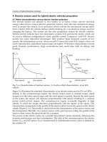
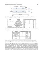
2.7.3 Simulation results
In order to verify the methods used to calculate the state-of-charge, internal voltage source,
and charging resistance calculations are compared to the data sheet values. The results can be
seen in Fig. 5 where the battery cell voltage is shown for different C-values (1 C is the nominal
discharge current of I
Bat,1,cell
= 7 A, which means that C/2 is equal to 3.5 A). It is seen that
the calculated voltages almost are identical to the data sheet values. It is also noticed that the
voltage is strongly depending on the current level and the delivered Ah, and that the voltage
drops significant when the battery is almost completely discharged.
8
Electric Vehicles – Modelling and Simulations
Electrical Vehicle Design and Modeling 9
0 1 2 3 4 5 6 7
2
2.5
3
3.5
4
Capacity Q
Bat,cell
[
Ah
]
C/5 Data sheet
C/5 Calculated
C/2 Data sheet
C/2 Calculated
1C Data sheet
1C Calculated
2C Data sheet
2C Calculated
Voltage v
Bat,cell
[
V
]
Fig. 5. Data sheet values (Saft, 2010) and calculations of the battery voltage during constant
discharge currents.
2.8 Boost converter
The circuit diagram of the boost converter can be seen in Fig. 6. The losses of the boost
4
%&
5
4%&
9
4WK%&
L
/
L
5)
9
'WK%&
'
%&
5
'%&
&
5)
Y
5)
&
%DW
Y
%DW
L
%&
Fig. 6. Electric circuit diagram of the boost converter.
converter are due to the switch resistance R
Q,BC
and threshold voltage V
Q,th,BC
and the
diodes resistance R
D,BC
and threshold voltage V
D,th,BC
. In order to simplify it is assumed
that the resistances and threshold voltages of the switch Q
BC
and diode D
BC
are equal, i.e.,
R
BC
= R
Q,BC
= R
D,RF
and V
th,BC
= V
Q,th,BC
= V
D,th,BC
. The power equations of the boost
converter are therefore given by
P
RF
= V
RF
i
RF
= P
BC
+ P
Loss,BC
(31)
P
BC
= V
Bat
i
BC
(32)
P
Loss,BC
= R
BC
i
2
RF
+ V
th,BC
i
RF
, (33)
9
Electrical Vehicle Design and Modeling
10 Will-be-set-by-IN-TECH
where P
RF
[
W
]
Input power of boost converter
P
BC
[
W
]
Output power of boost converter
P
Loss,BC
[
W
]
Power loss of boost converter
V
RF
[
V
]
Input voltage of boost converter
V
th,BC
[
V
]
Threshold voltage of switch and diode
R
BC
[
Ω
]
Resistance of switch and diode
i
RF
[
A
]
Input current of boost converter
i
BC
[
A
]
Output current of boost converter
2.9 Rectifier
In order to utilize the three phase voltages of the grid v
U
, v
V
,andv
W
they are rectified by a
rectifier as seen in Fig. 7. In the rectifier the loss is due to the resistance R
D,RF
and threshold
voltage V
D,th,RF
.
'
8
5
5)
9
WK5)
'
8
5
5)
9
WK5)
'
9
5
5)
9
WK5)
'
9
5
5)
9
WK5)
'
:
5
5)
9
WK5)
'
:
5
5)
9
WK5)
%RRVW
FRQYHUWHU
L
5)
L
/
&
5)
Y
5)
L
8
L
9
L
:
Y
9
Y
8
Y
:
*ULG 9HKLFOH
Fig. 7. Electric circuit diagram of the rectifier.
The average rectified current, voltage, and power are given by (Mohan et al., 2003)
i
RF
= I
Grid
3
2
(34)
V
RF
=
3
√
2
π
V
LL
−2R
RF
i
RF
−2V
th,RF
(35)
P
RF
= V
RF
i
RF
= P
Grid
− P
RF,loss
(36)
P
Grid
=
3
√
2
π
V
LL
I
RF
(37)
P
RF,loss
= 2R
RF
i
2
RF
+ 2V
th,RF
i
RF
, (38)
where I
Grid
[
A
]
Grid RMS-current
P
Grid
[
W
]
Power of three phase grid
P
loss,RF
[
W
]
Total loss of the rectifier
R
RF
[
Ω
]
Resistance of switch and diode
V
th,RF
[
V
]
Threshold voltage of switch and diode
10
Electric Vehicles – Modelling and Simulations
Electrical Vehicle Design and Modeling 11
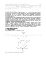
2.10 Simulation model
The models of each component of the power system in the electric vehicle have now been
explained. When combining all the sub models a model of the battery electric vehicle is
obtained. In Fig. 8 the implementation in a Matlab/Simulink environment can be seen. The
overall vehicle model includes the model of the forces acting on the vehicle (wind, gravity,
rolling resistance, etc.), and the individual components of the power train, i.e., transmission,
electric machine, inverter, battery, boost converter, rectifier. The wind speed v
wind
and road
angle α have been set to zero for simplicity. The input to the simulation model is a driving
cycle (will be explained in Section 4) and the output of the model is all the currents, voltages,
powers, torques, etc, inside the vehicle.
3. Design method
3.1 P arameter determination
The parameter determination of the components in the vehicle is an iterative process. The
parameters are calculated by using the models given in Section 2 and the outputs of the
Matlab/Simulink model shown in Fig. 8.
3.1.1 Battery
The maximum rectified voltage can be calculated from Equation 35 in no-load mode, i.e.,
V
RF,max
=
3
√
2
π
V
LL
=
3
√
2
π
400 V
= 540 V. (39)
In order to insure boost operation during charging the rectified voltage of the rectifier should
always be greater than this value. The required number of series connected cells is therefore
N
Bat,s
=
V
RF,max
V
Bat,cell,min
=
540 V
2.5 V
≈ 216 cells. (40)
The number of series connected cells N
Bat,s
is due to the voltage requirement of the battery
pack. However, in order to insure that the battery pack contains sufficient power and energy
it is probably not enough with only one string of series connected cells. The battery pack
will therefore consist of N
Bat,s
series connected cells and N
Bat,p
parallel strings. The number
of parallel strings N
Bat,p
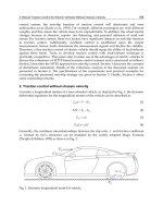
are calculated in an iterative process. The flow chart of the sizing
procedure of the battery electric vehicle can be seen in Fig. 9. In the “Initialization”-process the
base parameters are defined, e.g., wheel radius and nominal bus voltage, initial power ratings
of each component of the vehicle are given, and the base driving cycle is loaded into the
workspace of Matlab. In the “Is the minimum number of parallel strings obtained?”-decision
block it is verified if the minimum number of parallel strings that fulfills both the energy and
power requirements of the battery have been reached. If not a “Simulation routine”-process is
executed. This process are executed several times during the sizing procedure and its flow
chart is therefore shown separately in Fig. 9. This process consist of three sub-processes.
The first sub-process is “Design components”. In this process the parameters of each
component of the battery electric vehicle are determined, e.g., motor and power electronic
parameters. The next sub-process is the “Vehicle simulation”-process. In this process the
Simulink-model of the vehicle is executed due to the parameters specified in the previous
sub-process. In the third and last sub-process, i.e., the “Calculate the power and energy of each
component”-process, the energy and power of each component of the vehicle are calculated.
11
Electrical Vehicle Design and Modeling
12 Will-be-set-by-IN-TECH
Vehicle model
v_vehicle [km/h]
d_v_vehicle_dt [m/s^2]
v_wind [m/s]
alpha [rad]
f_t [N]
Transmission system
v_vehicle [km/h]
f_t [N]
w_s [rad/s]
tau_s [Nm]
Rectifier model
i_RF [A]
v_RF [V]
Inverter model
I_p_peak [A]
p_EM [W]
v_Bat [V]
i_Inv [A]
From
Workspace1
[t d_v_car_dt]
From
Workspace
[t v_car]
Electric machine
w_s [rad/s]
tau_s [Nm]
I_p_peak [A]
p_EM [W]
Electric auxiliary loads
v_Bat [V]
i_Aux [A]
Constant
0
Braking resistor
i_Aux [A]
i_Inv [A]
i_BC [A]
i_Bat_cha_max [A]
i_Bat [A]
Boost converter model
v_Bat [V]
SoC_Bat [−]
i_Bat_cha_max [A]
v_RF [V]
i_BC [A]
i_RF [A]
Battery model
i_Bat [A]
v_Bat [V]
SoC_Bat [−]
i_Bat_cha_max [A]
Fig. 8. Matlab/Simulink implementation of the battery electric vehicle.
12
Electric Vehicles – Modelling and Simulations
Electrical Vehicle Design and Modeling 13
The three sub-processes in the “Simulation routine”-process are executed three times in order
to make sure that parameters converges to the same values for the same input. After the
“Simulation routine”-process is finish the “Calculate number of parallel strings”-process is
applied. In this process the number of parallel strings N
Bat,p
is either increased or decreased.
When the minimum possible number of parallel strings that fulfills both the energy and power
requirements of the battery has been found the “Simulation routine”-process is executed in
order to calculate the grid energy due to the final number of parallel strings.
,QLWLDOL]DWLRQ
'HVLJQFRPSRQHQWV
9HKLFOHVLPXODWLRQ
&DOFXODWHWKHSRZHUDQG
HQHUJ\RIHDFKFRPSRQHQW
,VWKHPLQLPXPQXPEHURI
SDUDOOHOVWULQJVREWDLQHG"
IRUL
1R
&DOFXODWHQXPEHURI
SDUDOOHOVWULQJV
6LPXODWLRQURXWLQH
6LPXODWLRQURXWLQH
6LPXODWLRQURXWLQH
<HV
%HJLQ
(QG
Fig. 9. Sizing procedure of the battery electric vehicle.
In principle all the energy of a battery could be used for the traction. However, in order to
prolong the lifetime of the battery it is usually recommended not to charge it to more than
90 % of its rated capacity and not to discharge it below SoC
Bat,min
= 20 %, i.e., only 70 %
of the available energy is therefore utilized. In Fig. 10 it can be seen how the “Calculate
number of parallel strings”-process finds the minimum number of parallel strings N
Bat,p
that fulfills both the energy and power requirements. This process is a part of the sizing
procedure shown in Fig. 9. In Fig. 10(a) the minimum state-of-charge min(SoC
Bat
)isshown
and in Fig. 10(b) the maximum battery cell discharge current max(i
Bat,cell
)isshown. From
the figure it is understood that the first iteration is for N
Bat,p
= 10. However, both the
minimum state-of-charge and maximum discharge current are satisfying their limits, i.e.,
SoC
Bat,min
= 0.2 and I
Bat,max,cell
= 28 A, respectively. Therefore the number of parallel strings
is reduced to N
Bat,p
= 3 for iteration number two. However, now the state-of-charge limit is
exceeded and therefore the number of parallel strings is increased to N
Bat,p
= 8 for iteration
three. This process continuous until iteration number six where the number of parallel strings
settles to N
Bat,p
= 6, as this is the minimum number of parallel strings which ensures that
both the state-of-charge and maximum current requirements are fulfilled.
13
Electrical Vehicle Design and Modeling