Electric Vehicles Modelling and Simulations Part 7 pot

FPGA Based Powertrain Control for
Electric Vehicles 11
30 15 20 25250
cycles
2500 cycles
ADC Interface
(Currents Acquisiton)
TClarke
+TPark
IFOC
Start
IFOC
Start
PI
Rect2Polar
SVPWM

30 15 20 25250
MC
(Left)
MC
(Right)
340 cycles
cycles
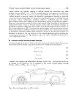
Fig. 5. Latency i ntroduced by the MC sub-modules (the main cl ock in the FPGA has a
frequency of 50MHz, thus 2500cyces
⇔ 50us)
Type Module Slices Mul. BRAM. FMax(MHz)
Motor Control
SVPWM 316 1 1 86
TClark+TPark 212 2 1 78

2xPI’s + Cart2Polar 1012 6 1 92
Field Weakening 59 2 1 125
Sensor Interface
ADC Interface (ADS7818) 47 190
Quadrature Decoder 37 134
Protections Protections 75 183
Soft Processor PicoBlaze + SPI + UART + 501 3 85
Table 1. Resource utilization of the main IP cores (Note: the design tool was the ISE WebPack
8.2.03i, FPGA family: Spartan 3, Speed Grade: -5).
Module Num. Instances Slices Mul.
Motor Control(MC) 2 3198 22
Sensor Interface 2 168
Protections 1 75
Soft Processor 1 501
Others 1 789
Total
4731 22
(61%) (92%)
Table 2. Resource utilization of the XC3S1000 FPGA used to control the uCar prototype
(Note: the design tool was the ISE WebPack 8. 2.03i, FPGA family: Spartan 3, Speed Grade:
-5).
representing 14% of the 2500 cycles as sociated with the MC minimum execution rate (20kHz).
This minimum rate is the result of the energy dissipation limits in the power semiconductors,
which, in hard-switching, high current tr action applications, is normally constrained to a
maximum of 20kHz switching frequency. Albeit the MC modules have been specifically
developed for electric traction applications, with the 20 kHz update rate limit, the low value of
latency permits a higher execution rate, u p to 147 kHz. This feature enables the MC modules
to be reused in other industrial applications, where a high-bandwidth control of torque and
169
FPGA Based Powertrain Control for Electric Vehicles

12 Will-be-set-by-IN-TECH
(a) Motor controller and SVPWM configuration (b) Debug screen
(c) Telemetry plot for current regulation (d) Telemetry plot for motor position
Fig. 6. User interfaces of the s oftware developed to configure and debug the EV controller.
speed is necessary. Figure 5 also shows the parallel processing capabilities of FPGA, which
allows multiple instantiations of the MC to run simultaneously, independently and without
compromising the bandwidth of other modules.
A summary of the resource utilization in the IP cores implementation, such as slices, dedicated
multipliers and Block Ram (BRAM), is presented in Tables 1 and 2 . The two Motor Controllers
instantiated in control unit are the most demanding on the FPGA resources, requiring 44% of
the slices and 92% of the dedicated multipliers available on the chip. Although there are a
considerable number of slices available (39%), the low number of free multipliers prevents the
inclusion of additional MC, presenting a restriction for future improvements in this FPGA; in
other words, such improvements would need an FPGA with more computational resources,
thus more costly. In addition to the MC, there are also others modules to perform auxiliary
functions (sensor interface, protections, soft processor), described in the previous section, and
which consume 17% of the FPGA area.
170
Electric Vehicles – Modelling and Simulations
FPGA Based Powertrain Control for
Electric Vehicles 13
DC Bus
Capacitors
Current
Sensors
MOSFET
Drivers
12x Power
MOSFETs
Digilent

Starter Board
Expansion Boards
[analog and digital
interface]
Board Power Supply
[48Vo 12V,5V
conversion]
FPGA Control System
DC/AC Power Converters
4x12V Lead Acid Batteries
Powertrain for each front wheel
AC Induction
Motor
[2kW @ 1500rpms]
Single-Gear
Transmission
(7:1)
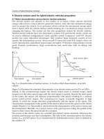
uCar EV Prototype
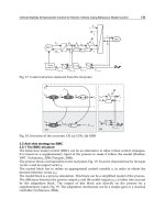
Fig. 7. uCar electric vehicle prototype.
3.4 Configuration software
During the EV development, it is necessary to exchange configuration and debugging data
with the FPGA control unit. To this aim, we built a graphical application based on the
cross-platform wxWidgets library, whose main user interfaces are depicted in Fig. 6. This
application, running on a convention co mputer, establishes a communication channel with the
tasks 4 and 5, briefly described in Section 3.1.4. Based o n this interface, the EV d esigner has the
possibility to change the EV control parameters associated with the motor controller (current
and flux limits, pair of poles, etc.), peripherals (encoder pulses), modulation ( switching
frequency, dead-times, etc.), among other mo dules. F or debugging the controller we also have
a datalogger interface (Fig. 6(c)), which enables the real-time acquisition of the EV controller
variables, like the motor currents, voltages and mechanical position, providing an effective

mechanism to inspect the performance of the control loops d uring fast transients and aid the
controller tuning process.
3.5 Experimental results
In order to evaluate the control system discussed in the previous sections, an EV prototype,
named uCar, was built to accommodate the electric powertrain (see Fig. 7). The vehicle is
based on a two-seater quadricycle, manufactured by the MicroCar company, and is very
popular among elderly people of southern Europe, mainly due to non-compulsory driving
license. The original propulsion structure, based on the internal combustion engine, was
replaced by a new electric powertrain composed by two electric motors (26 Vrms, 2.2 kW
@ 1410 rpm), each one coupled to the front wheels by single gear (7 : 1) transmissions. Due to
low cost, lead acid batteries (4x12V@110Ah) were selected as the main energy storage of the
EV, providing a range of 40 km per charge, a sufficient autonomy for urban driving. After the
conversion, the uCar prototype weights 590 kg and reaches a top speed of 45 km/h.
171
FPGA Based Powertrain Control for Electric Vehicles
14 Will-be-set-by-IN-TECH
350 400 450 500 550 600 650 700 750 800
−10
0
10
20
30
40
time [s]
Speed [km/h]
350 400 450 500 550 600 650 700 750 800
0
2000
4000
6000

time [s]
Power [W]
(a) regenerative braking OFF
1300 1400 1500 1600 1700 1800 1900 2000 2100 2200
−10
0
10
20
30
40
time [s]
Speed [km/h]
1300 1400 1500 1600 1700 1800 1900 2000 2100 2200
−2000
0
2000
4000
6000
time [s]
Power [W]
(b) regenerative braking ON
Fig. 8. Experimental results of a typical driving cycle performed by the uCar inside the
university campus, with and without regenerative braking active.
All the powertrain control functions of the EV are concentrated on the Digilent Spartan
3 Start Board, containing, besides the XC3S1000 FPGA, several useful peripherals such as
flash memory (2 Mbit) for s toring data, serial interface for communications and 4 expansion
ports for I/O with the FPGA. To extend the functionalities of these main peripherals, two
additional boards were constructed and connected to the main board, containing analog to
digital converters (TIADS7818 and TIADS7848) to allow the acquisition of analog variables,
and voltage level shifters (3.3

↔ 5.0V) t o perform the interface with the external digital I/O.
This EV controller interacts with two DC/AC power converters, featuring 120Arms@30Vr ms
and 20kHz s witching f requency, in order t o regulate the current and voltage delivered to the
electric motors, as discussed in the previous sections.
To validate the experimental p erformance of the uCar, several roadtests we re conduced inside
the FEUP university campus, characterized by low speed driving cycles, similar to urban
conditions (see Fig. 8). From these ro adtests, we selected two representative cycles for assess
the influence of the regenerative braking in the energy consumption of the uCar. In the first
situation, with the regenerative braking disabled, the vehicle travels approximately 2.36 km
and shows consumption metrics close to 100 Wh/km (see Table 3). On the other hand, when
the reg. braking is active the EV consumption decreases 13.2%, to 86.8 Wh/km, representing
an important contribute to i ncrease the EV range per charge.
172
Electric Vehicles – Modelling and Simulations
FPGA Based Powertrain Control for
Electric Vehicles 15
Mode Distance Energy Energy Consump. Max. Min.
Delivered Regenerated Power Power
Reg. OFF 2.37km 236.7 W.h 0W.h 99.9 Wh/km 6.3 kW 0kW
Reg. ON 4.26km 417.6 W.h 48.3W.h 86.8 Wh/km 6.3 kW -3.5 kW
Table 3. Performance metrics of the uCar over the driving cycles described in Fig. 8.
854 856 858 860 862 864 866 868 870 872
0
10
20
30
40
50
60
70

80
time [s]


Speed [km/h]
I
q
[A]
I
d
[A]
f
slip
[Hz]
m
SVPWM
[%]
(a) Acceleration + Field Weakening
1806 1808 1810 1812 1814 1816 1818
−40
−20
0
20
40
60
80
100
time [s]

Speed [km/h]
I
q
[A]
I
d
[A]
f
slip
[Hz]
m
SVPWM
[%]
(b) Regenerative braking
854 856 858 860 862 864 866 868 870 872
−10
0
10
20
30
40
50
60
time [s]


V
dc
[V]
I

dc
[A]
10*Power [kW]
(c) DC Bus variables (acceleration)
1806 1808 1810 1812 1814 1816 1818
−30
−20
−10
0
10
20
30
40
50
60
time [s]


V
dc
[V]
I
dc
[A]
10*Power [kW]
(d) DC Bus variables (reg. braking)
Fig. 9. Detailed view of the uCar (left motor) results during accelerating, field weakening and
regenerative braking.
To further validate the EV control unit performance, Fig. 9 show the detailed results of the
left motor controller for tree different operating modes: acceleration, field weakening and

regenerative braking. The data depicted in these figures was acquired with the controller
internal datalogger, which enable us to keep track of the most relevant EV variables, such
as: mechanical (motor speed), energy source (voltage, current and power) and the motor
controller ( torque (i
q
)andflux(i
d
) currents, modulation index (m) and the slip frequency
( f
sli p
)) variables. During the acceleration mode (Fig.9(a), 9(c)), performed with the throttle at
100%, the i
q
and i
d
currents are set at the maximum value in order to extract the maximum
motor torque and vehicle acceleration ( 2 .2km/h/s). When the EV reaches 18km/h the mo tor
voltage saturates at 83% and the flux current is reduced to allow the vehicle to operate in
the field weakening area, with a power consumption of 2.5kW per motor. In fact, analyzing
the evolution of the power supplied by the batteries during the experimental driving cycles
(Fig. 8), it is interesting to note that the electric motors spend most of the time operating in
this field weakening zone. Fig. 9(b) and 9(d) shows the detailed results of third EV operation
173
FPGA Based Powertrain Control for Electric Vehicles
16 Will-be-set-by-IN-TECH
mode: the re generative braking. In the depicted manoeuvre, the driver is requesting a torque
current of -25A to decelerate the vehicle from 30 km/h to 5 km/h in 10s, which enable a
conversion of 1kW peak power and emphasizing one of the most promising features in EVs:
energy recovering during braking.
4. Conclusion

In this article an FPGA based solution for the advance control of multi-motor EVs was
proposed. The design was build around a powertrain IP Core library containing the most
relevant functions for the EV operation: motor torque and flux regulation, energy loss
minimization and vehicle safety. Due to the parallel, modularity and reconfigurability features
of FPGAs, this library can be reused in the development of several control architectures
that best suits the EV powertrain configuration (single or multi-motor) and functional
requirements. As proof of concept, the powertrain library was employed in the design
of minimal control system for a bi-motor EV prototype and implemented in a low cost
Xilinx Spartan 3 FPGA. Experimental verification of the control unit was provided, showing
reasonable consumption metrics and illustrating the energy benefits from regenerative
braking.
In future works, we are planning the inclusion, in the powertrain library, of active torque
methods in order to improve the handling and safety of multi-motor EVs. On the
technological level, we also intent to validate the library on EV prototypes with 4 in-wheel
motors.
5. References
Actel (2010). Fusion Family of Mixed Signal F PGAs datasheet.
Araujo, R. E. (1991). Control System of Three-phase Induction Motor based on the Principle of Field
Orientation, Master thesis, Faculdade de Engenharia da Uni versidade do Porto.
Araujo, R. E. & Freitas, D. S. (1998). The Development of Vector Control Signal Processing
Blockset for Simulink: Philosophy and Implementation, Proceedings of the 24th Annual
Conference of the IEEE Industrial Electronics Society.
Araujo, R. E., Oliveira, H. S., Soares, J. R., Cerqueira, N. M. & de Castro, R. (2009). Diferencial
Electronico. Patent PT103817.
Araujo, R. E., Ribeiro, G., de Castro, R. P. & Oliveira, H. S. (2008). Experimental evaluation of
a loss-minimization control of induction motors used in EV, 34th Annual Conference
of IEEE Industrial Electronics, Orlando, FL, pp. 1194–1199.
Barat, F., Lauwereins, R. & Deconinck, G. (2002). Reconfigurable instruction set processors
from a hardware/software perspective, IEEE Transactions on Software Engineering
28(9): 847–862.

Cecati, C. (1999). Microprocessors for power electronics and electrical drives applications,
IEEE Industrial Electronics Society Newsletter 46(3): 5–9.
Cerqueira, N. M., Soares, J. R., de Castro, R. P., Oliveira, H. S. & Araujo, R. E. (2007).
Experimental evaluation on parameter identification of in duction motor using
continuous-time approaches, Internation al Conference on Power Engineering, Energy and
Electrical Drives,Setubal,Portugal.
Chan, C. C. (2007). The State of the Art of Electric, Hybrid, and Fuel Cell Vehicles, Proceedings
of the IEEE 95(4): 704–718.
174
Electric Vehicles – Modelling and Simulations
FPGA Based Powertrain Control for
Electric Vehicles 17
de Castro, R. (2010). Main Solutions to the Control Allocation Problem, Technical r eport,
Universidade do Porto.
de Castro, R., Araujo, R. E. & Freitas, D. (2010a). A Single Motion Chip for Multi-Motor
EV Control, 10th International Symposium on Advanced Vehicle Control (AVEC),
Loughborough, UK.
de Castro, R., Araujo, R. E. & Freitas, D. (2010b). Reusable IP Cores Library for EV Propulsion
Systems., IEEE International Symposium on Industrial Electronics, Bari, Italy.
de Castro, R., Araujo, R. E. & Oliveira, H. (2009a). Control in Multi-Motor Electric Vehicle
with a FPGA platform, IEEE International Symposium on Industrial Embedded Systems,
Lausanne, Switzerland, pp. 219–227.
de Castro, R., Araujo, R. E. & Oliveira, H. (2009b). Design, Development and Characterisation
of a FPGA Platform for Multi-Motor Electric Vehicle Control, The 5th IEEE Vehicle
Power and Propulsion Conference, Dearborn, USA.
Delli Colli, V., Di Stefano, R. & Marignetti, F. (2010). A System-on-Chip Sensorless Control for
a Permanent-Magnet Synchronous Motor, IEEE Transactions on Industrial Electronics
57(11): 3822–3829.
Fasang, P. P. (2009). Prototyping for Industrial Applications, IEEE Industrial Electronics
Magazine 3( 1): 4–7.

Geng, C., Mostefai, L., Denai, M. & Hori, Y. (2009). Direct Yaw-Moment Control of an
In-Wheel-Motored Electric Vehicle Based on Body Slip Angle Fuzzy Observer, IEEE
Transactions on Industrial Electronics 56(5): 1411–1419.
Guzman-Miranda, H., Sterpone, L., Violante, M., Aguirre, M. & Gutierrez-Rizo, M. (2011).
Coping With the Obsolescence of Safety - or Mission-Critical Embedded Systems
Using FPGAS, IEEE Transactions on Industrial Electronics 58(3): 814 – 821.
He, P., Hori, Y., Kamachi, M., Walters, K. & Yoshida, H. (2005). Future motion control to be
realized by in-wheel motored electric vehicle, 31st Annual Conference of IEEE Industrial
Electronics Society.
Hori, Y. (2004). Future vehicle driven by electricity and control - Research on
four-wheel-motored UOT Electric March II, IEEE Transactions on Industrial Electronics
51(5): 954–962.
Idkhajine, L., Monmasson, E., Naouar, M. W., Prata, A. & Bouallaga, K. (2009). Fully Integrated
FPGA-Based Controller for Synchronous Motor Drive, IEEE Transactions on Industrial
Electronics 56(10): 4006–4017.
Jung Uk, C., Quy Ngoc, L. & Jae Wook, J. (2009). An FPGA-Based Multiple-Axis Motion
Control Chip, IEEE Transactions on Industrial Electronics 56(3): 856–870.
Kazmierkowski, M., Krishnan, R. & Blaabjerg, F. (2002). Control in Power Electronics: Selected
Problems, Academic Press.
Lopez, O., Alvarez, J., Doval-Gandoy, J., Freijedo, F. D., Nogueiras, A., Lago, A. & Penalver,
C. M. (2008). Comparison of the FPGA Implementation of Two Multilevel Space
Vector PWM Algorithms, IEEE Transactions on Industrial Electronics 55(4): 1537–1547.
MathWorks (2010). Simulink HDL Coder 2.0 User Guide.
Monmasson, E. & Cirstea, M. N. (2007). FPGA Design Methodology for Industrial Control
Systems-A Review, IEEE Transactions on Industrial Electronics 54(4): 1824–1842.
Naouar, M. W., Monmasson, E., Naassani, A. A., Slama-Belkhodja, I. & Patin, N.
(2007). FPGA-Based Current Controllers for AC Machine Drives-A Review, IEEE
Transactions on Industrial Electronics 54(4): 1907–1925.
Novotny, D. & Lipo, T. (1996). Vector control and dynamics of AC drives, Oxford University Press.
175

FPGA Based Powertrain Control for Electric Vehicles
18 Will-be-set-by-IN-TECH
Oliveira, H. S., Soares, J. R., Cerqueira, N. M. & de Castro, R. (2006). Veiculo Electrico de
Proximidade com Diferencial Electronico, Licenciatura thesis, Universidade do Porto.
Rahul, D., Pramod, A. & Vasantha, M. K. (2007). Programmable Logic Devices for Motion
Control-A Review, IEEE Transactions on Industrial Electronics 54(1): 559–566.
Rodriguez-Andina, J. J., Moure, M. J. & Valdes, M. D. (2007). Features, Design Tools,
and Application Domains of FPGAs, IEEE Transactions on Industrial Electronics
54(4): 1810–1823.
Seo, K., Yoon, J., Kim, J., Chung, T., Yi, K . & Chang, N. (2010). Coordinated implementation
and processing of a unified chassis control algorithm with multi-central processing
unit, Proceedings of the Institution of Mechanical Engineers, Part D: Journal of Automobile
Engineering 224(5): 565–586.
Takahashi, T. & Goetz, J. (2004). Implementation of complete AC servo control in a low
cost FPGA and subsequent ASSP conversion, Nineteenth Annual IEEE Applied Power
Electronics Conference and Exposition.
Tazi, K ., Monmasson, E . & Louis, J . P. (1999). Description of an entirely reconfigurable
architecture dedicated to the current vector control of a set of AC machines, The 25th
Annual Conference of the IEEE Industrial Electronics Society.
van Zanten, A. T. (2002). Evolution of electronic control systems for improving the vehicle
dynamic behavior, P roceedings of the International Symposium on Advanced Vehicle
Control (AVEC), Hiroshima, Japan, p p. 7–15.
Winters, F., Nicholson, R., Young, B., Gabrick, M. & Patton, J. (2006). FPGA Considerations
for Automotive Applications, SAE 2006 World Congress and Exhibition,Detroit,MI.
Xilinx (2005). System Generator User Guide.
Xilinx (2010). PicoBlaze 8-bit Embedded Microcontroller User Guide.
Ying-Yu, T. & Hau-Jean, H. (1997). FPGA realization of space-vector PWM control IC for
three-phase PWM inverters, Power Electronics, IEEE Transactions on 12(6): 953–963.
Zeraoulia, M., Benbouzid, M. E. H. & Diallo, D. (2006). Electric M otor Drive Selection Issues
for HEV Propulsion Systems: A Comparative Study, IEEE Transactions on Vehicular

Technology 55(6): 1756–1764.
176
Electric Vehicles – Modelling and Simulations
8
Global Design and Optimization of
a Permanent Magnet Synchronous Machine
Used for Light Electric Vehicle
Daniel Fodorean
Technical University of Cluj-Napoca, Electrical Engineering Department
Romania
1. Introduction
One of the most common problems of modern society, these days, particularly for
industrialized countries, is the pollution (Fuhs, 2009; Ehsani et al., 2005; Vogel, 2009; Ceraolo
et al., 2006; Chenh-Hu & Ming-Yang, 2007; Naidu et al., 2005). According to several studies,
the largest share of pollution from urban areas comes from vehicle emissions and because of
this explosive growth of the number of cars. The pollution effect is more and more obvious,
especially in large cities. Consequently, finding a solution to reduce (or eliminate) the
pollution is a vital need. If in public transports (trains, buses and trams) were found non-
polluted solutions (electrical ones), for the individual transport the present solutions can not
yet meet the current need in autonomy. Even though historically the electric vehicle
precedes the thermal engine, the power/fuel-consumption ratio and the reduced time to
refill the tank has made the car powered by diesel or gasoline the ideal candidate for private
transport. Although lately there were some rumors regarding the depletion of fossil
resources, according to recent studies, America's oil availability is assured for the next 500
years (Fuhs, 2009; Ehsani et al., 2005). So, the need of breathing clean air remains the main
argument for using electric vehicles (EV). However, all over the world, one of the current
research topics concerns the use of renewable energy sources and EVs.
With regard to automobiles, there have been made several attempts to establish a maximum
acceptable level of pollution. Thus, several car manufacturers have prepared a declaration of
Partnership for a New Generation of Vehicles (PNGV), also called SUPERCAR. This concept

provides, for a certain power, the expected performance of a thermal or hybrid car.
Virtually, every car manufacturer proposes its own version of electric or hybrid car, at
SUPERCAR standard, see Table 1 (Fuhs, 2009).
Of course, at concept level, the investment is not a criterion for the construction of EVs, as in
the case of series manufacturing (where profits are severely quantified). For example,
nowadays the price of 1 kW of power provided by fuel cell (FC) is around 4,500 €; thus, a FC of
100 kW would cost 450,000 € (those costs are practically prohibitive, for series manufacturing).
By consulting Table 1, it can be noticed the interest of all car manufacturers to get a reduced
pollution, with highest autonomy. Nowadays, the hybrid vehicles can be seen on streets.
Although the cost of a hybrid car is not much higher than for the classical engine (about 15-
25% higher), however, the first one requires supplementary maintenance costs which cannot
be quantified in this moment.

Electric Vehicles – Modelling and Simulations
178
Conce
p
t Cars Technical Data Performances
AUDI metroproject
quattro
turbocharged four-cylinder engine and an
electric machine of 30 kW; lithium-ion battery
maximum ran
g
e on electric-onl
y
of
100 km; 0-100 km/h in 7.8 s; maximum
s
p

eed 200 km/
h
BMW x5 hybrid SUV
for 1000 rpm, there is a V-8 en
g
ine providin
g

1000 Nm; the electric motor
g
ives 660 Nm
fuel econom
y
is improved b
y
an
estimated 20%.
CHRYSLER eco
vo
y
a
g
er FCV
propulsion of 200 kW; h
y
dro
g
en is feed to a
PEM fuel cell
(

FC
)
ran
g
e of 482 km and a 0–60 km/h in
less than 8 s.
CITROËN c-cactus
h
y
brid
diesel en
g
ine provides 52 kW and the electric
motor
g
ives 22 kW
fuel consumption is 2.0 L/100 km;
maximum speed is 150 km/
h

FORD hySeries EDGE
Li-ion batter
y
has maximum power of
130 kW, and the FC provides 35 kW
ran
g
e of 363 km (limited b
y
the amount

of h
y
dro
g
en for the FC)
HONDA FCX
electric vehicle with 80 kW propulsion en
g
ine,
combinin
g
ultracapacitors (UC) and PEM FC
55% for overall efficienc
y
, drivin
g

ran
g
e of 430 km
HYUNDAI I-blue
FCV
FC stack produces 100 kW; there is a 100 kW
electric machine (front wheels) and 20 kW
motor for each rear wheel
estimated range is 600 km
JEEP renegade diesel–
electric
1.5 L diesel en
g

ine provides 86 kW and is
teamed with 4 electric motors (4WD) of
85 kW combined power
the diesel provides ran
g
e extension up
to 645 km beyond the 64 km electric-
onl
y
ran
g
e (diesel fuel tank holds 38 L)
KIA FCV
a 100 kW FC suppliss a 100 kW front wheel
electric motor, while the motor driving the
rear wheels is 20 kW
range is stated to be 610 km
MERCEDES BENZ s-
class direct hybrid
3.5 L (V-6)
g
asoline en
g
ine with
motor/generator combined power of 225 kW
and combined torque of 388 Nm
acceleration time from 0-100 km/h in
7.5 s
MITSUBISHI pure EV Li-ion battery and wheel-in-motors of 20 kW
150 k

g
Li-ion batter
y

g
ive a ran
g
e of
150 km (2010 prospective range of
250 km
OPEL flextreme
a series h
y
brid confi
g
uration (with diesel
engine) with Li-ion battery; the electric motor
has peak power of 120 kW
fuel consumption of 1.5 L/100 km;
electric only mode has range of 55 km
PEUGEOT 307 hybrid it is diesel/electric hybrid automobile
the estimated fuel econom
y
is 82 mp
g
;
this is a hybrid that matches the PNGV
g
oals
SUBARU G4E five passengers EV, using Li-ion batteries

drivin
g
ran
g
e is 200 km; the batter
y
can
be fully charged at home in 8 h (an 80%
char
g
e is possible in 15 min)
TOYOTA 1/X plug-in
hybrid
thermal en
g
ine 0.5 L, with a hu
g
e reduction
of mass to 420 kg (use of carbon fiber
composites, althou
g
h expensive)
low mass also means low en
g
ine power
and fuel consumption
VOLKSWAGEN Blue
FC
a 12 kW FC mounted in the front char
g

es
12 Li-ion batteries at the rear; The 40 kW
motor is located at the rear
the electric-onl
y
ran
g
e is 108 km; top
speed is 125 km/h, and the acceleration
time from 0-100 km/h is 13.7 s
VOLVO recharge
series h
y
brid with lithium pol
y
mer batteries;
the engine is of 4-cylinder type with1.6 L; it
has 4 electric wheels motors (AWD)
electric-onl
y
ran
g
e is 100 km; for a
150 km trip, the fuel economy is
1.4 L/100 km
Table 1. Several types of hybrid vehicle concepts.
Some predictions on the EV’s were considered by (Fuhs, 2009). In the nearest future the
thermal automobiles number will decrease, while the hybrid ones are taking their place. By
2037 the fully electric vehicle (called kit car) will replace the engine and then, after a fuzzy
period all vehicles will be powered based on clean energy sources, when a new philosophy

of building and using the cars will be put in place.
So, one of the challenges of individual transport refers to finding clean solutions, with
enhanced autonomy (Ceraolo et al., 2006; Chenh-Hu & Ming-Yang, 2007; Naidu et al., 2005).
Global Design and Optimization of
a Permanent Magnet Synchronous Machine Used for Light Electric Vehicle
179
This is the motivation of this research work. For that, an electric scooter will be studied from
the motorization, supplying and control point of view. The global steps of the design
process will be presented here. Firstly, the considered load and expected mechanical
performances will be introduced. The electromagnetic design of the electrical motor, capable
to fulfill the mechanical performances, will be presented too. The obtained analytical
performances should be validated; for that, the finite element method will be used. Also, the
machine optimization will fulfill the global designing process of the electrical machine.
2. Design of studied electrical machine
The research study presented here concerns the design of a three phase permanent magnet
synchronous machine (PMSM) used for the propulsion of an electric scooter. It is widely
recognized that the common solution, the dc motor, has usually poor performances against
ac motor. However, for low small power electrical machines, this advantage is not always
obvious. Also, a special attention should be paid for the efficiency and power factor of ac
machines. This will be analyzed here. The validation of the obtained results will be made
based on finite element method (FEM) analysis. The goal is to increase the autonomy of the
light electric vehicle, based on a PMSM, with a proper control, and after the optimization of
the designed machine.
The analytical approach, employed here, can be used for any type of electric vehicle. First of
all, for a given maximum load, it will be established the necessary power needed for the
propulsion of the vehicle. Secondly, the main steps in the design process of the studied
machine will be given. Next, the energetic performances and electro-mechanical
characteristics will be presented. The validation of the analytical obtained results is made
based on finite element method (FEM). By means of numerical computation, it will be
demonstrated that a unity power factor control is possible when using ac machines, by

employing a field oriented control strategy. The optimization of the studied machine will be
realized based on gradient type algorithm and the obtained results will show the benefits of
using a PMSM for the propulsion of the light electric vehicle.
2.1 The needed mechanical performances
The maximum speed and weight of the vehicle are 12 km/h and 158 kg, respectively. The
considered vehicle has 4 tires of 11 inches in diameter. The vehicle dimensions are: 1290 mm
in length, 580 mm in width and 1150 mm in height. The vehicle will be supplied from a
battery of 24 Vcc.
First of all, it is needed to compute the output power of the electric motor which is capable
to run the vehicle. Since the mechanical power is the product between the mechanical torque
and angular speed, it is possible to establish the speed of the vehicle at the wheel:
n

=v∙60/(π∙D

) (1)
where n
t
is the velocity measured at the vehicle’s wheels (measured in min-1), v is the vehicle
speed (in m/s), D
t
is the outer diameter of the wheel (the tire height included, in m). The
resulted velocity is n
t
=244.4 min
-1
. From mechanical and controllability considerations, it is
desirable to have an electric motor operating at higher speed, so it is considered a gear ratio of
6.1 to 1. Thus the electric motor rated speed is imposed at 1500 min
-1

.
Next, the rated torque has to be established. Since the motor torque is proportional to the
wheel radius and the force acting on it, one should determine the force involved by the

Electric Vehicles – Modelling and Simulations
180
vehicle’s weight and rolling conditions. The electric motor has to be capable to produce a
mechanical force to balance all other forces which interfere in vehicle’s rolling. Thus, the
motor force is:
F

=F

+F

+F

+F

+F

(2)
where F
acc
is the acceleration force, F
h
is the climbing force, F
d
is the aerodynamic drag force,
F

w
is a resistive force due to the wind, and F
r
is the rolling force.
Since the vehicle studied here is not for racing, and will be controlled to start smoothly, no
acceleration constraints are imposed.
When the vehicle goes hill climbing, based on angle of incline θ, the climbing force is:
F

=M

∙g∙sin(θ) (3)
where M
tot
, is the total mass of the vehicle (in kg), g is the gravitational constant (9.8 m/s
2
).
Usually, the degree of incline is given in percentage. For this special electric scooter it is
considered a maximum 8% degree of incline. 1% degree of incline represents the ratio of
1 meter of rise, on a distance of 100 meters. Thus, 1%=atan(0.01)=0°34’ (zero degrees and
34 minutes). For an incline of 8%, the angle is 4°34’ (or 4.57 degrees).
The drag force takes into account the aerodynamics of the vehicle. This force is proportional
with the square of the speed, the frontal area of the vehicle (A
fr
, here 0.668 m
2
) and the
aerodynamic coefficient, k
d
, (empirically determined, for each specific vehicle (Vogel, 2009)):

F

=A

∙v

∙g∙k

(4)
The resistant force due to wind, cannot be precisely computed. It depends on various
conditions, like (for common automobiles) the fact that windows are entirely or partially
open etc Also, the wind will never blow at constant speed. However, an expression,
determined empirically, which will take into account the speed of wind, v
w
, can be written
as (Vogel, 2009):
F

=0.98∙
(
v

/v
)

+0.63∙
(
v

/v

)
∙k

−0.4∙
(
v

/v
)
∙F

(5)
where k
rw
is the wind relative coefficient, depending on the vehicle’s aerodynamics, (here is
1.6).
The resistant force due to rolling depends on the hardness of the road’s surface, being
proportional with the weight of the vehicle and the angle of incline:
F

=k

∙M

∙g∙cos(θ) (6)
(here, the road surface coefficient, k
r
, is 0.011).
A more precise computation of the rolling resistant force could take into account also the
shape and the width of the tires, but these elements are not critical at low speeds, like in this

case.
After the computation of the resistant forces, it can be determined the needed torque at the
wheel, see Table 2, and finally the rated torque of the electrical machine.
For this specific value of the torque at the wheel, a power of 505.1 W is required.
Nevertheless, for small power electrical traction systems, the efficiency is quite poor. Here,
the efficiency is estimated at 75%. This means that the output power of the electrical motor,
capable to operate in the specified road/mechanical conditions, it has to be at least of
673.5 W. Thus, rounding the power, it is obtained a 700 W electrical machine.
Global Design and Optimization of
a Permanent Magnet Synchronous Machine Used for Light Electric Vehicle
181
It is now possible to identify the mechanical characteristics of the electrical machines. Two
traction motors are considered, with a gear ratio of 6.1 to 1. Thus, the rated mechanical
characteristics for one motor are: 350 W, 1500 rpm, 2.2 N
.
m.

F
h
(N) F
d
(N) F
w
(N) F
r
(N) F
m
(N)
torque at the
wheel (N

.
m)
123.5 0.026 0.667 16.98 141.2 19.73
Table 2. Computed resistant forces and the torque at the wheel.
2.2 Electromagnetic design of the PMSM
The permanent magnet synchronous machine (PMSM) has to provide a maximum power
density. For that, good quality materials should be used. The permanent magnet (PM)
material is of Nd-Fe-B type, with 1.25 T remanent flux density. The steel used for the
construction of PMSM is M530-50A. The material characteristics are presented in Fig. 1.






Fig. 1. The PM and steel characteristics used as the active part’s materials of the PMSM.
-10 -8 -6 -4 -2 0
x 10
5
0
0.5
1
1.5
magnetic field intensity (A/m)
flux density (T
)
Magnetic characteristic of the PM material: Nd-Fe-B N38SH
PM operating point
0 2000 4000 6000 8000 10000 12000 14000 16000 18000
0

0.5
1
1.5
2
B(H) characteristic of the M530-50A steel
magnetic field intensity (A/m)
flux density (T)
0 0.5 1 1.5 2
0
20
40
60
80
100
120
M530-50A Steel
specific material losses (W/kg)
flux density (T)


50Hz
100Hz
200Hz
400Hz

Electric Vehicles – Modelling and Simulations
182
For the PM, the N38SH material was use. This rear earth magnet can be irreversible
demagnetized starting from 120°C. The 1.25 T remanent flux density (at 20°C) is however
affected with the temperature increase. In order to compute the real value of the PM’ s

remanent flux density, for a temperature derivative coefficient of 0.1% and for an increase in
temperature of 110 K, the rated operating point of the PM is 1.11 T (based on the
mathematical expression X
°
=X
°
∙
(
1−α

∙ΔT
)
).
In order to obtain a smooth torque wave, a fractioned winding type is used. Thus, the
PMSM has 8 pair of poles and 18 slots. The geometry of the PMSM, the winding
configuration and the obtained phase resultant vectors are shown in Fig. 2.
The design approach is based on the scientific literature presented in (Pyrhonen et al., 2008;
Fitzgerald et al., 2003; Huang et al., 1998). The output power (measured in W) of an electric
machine, when the leakage reactance is neglected, is proportional with the number of
phases of the machine, n
ph
, the phase current, i(t), and the inducted electromotive force
(emf), e(t):
P

=η∙



∙


e
(
t
)
∙i
(
t
)
dt =


η∙n

∙k

∙E

∙I

(7)
where T is the period of one cycle of emf, E
max
, and I
max
represent the peak values of the emf
and phase current, k
p
is the power coefficient, and η is the estimated efficiency.
The peak value of the emf is expressed by introducing the electromotive force coefficient, k

E
:
E

=k

∙N

∙B

∙D

∙L

∙
f

p

(8)
where N
t
is the number of turns per phase, B
gap
and D
gap
are the air-gap flux density and
diameter, L
m
is the length of the machine, f

s
is the supplying frequency and p is the number
of pole pairs.
By introducing a geometric coefficient, k
L
=L
m
/D
gap
, and a current coefficient (related to its
wave form) k
i
=I
max
/I
rms
, and defining the phase load ampere-turns,
A

=2/π∙N

∙I

/D

(9)
it is possible to define the air-gap diameter of the machine:

out
3

gap
ph t e i p L
g
ap s
2pP
D
π nAkkkkη Bf
⋅⋅
=
⋅⋅⋅⋅⋅⋅⋅⋅ ⋅
(10)
Based on the type of the current wave form, it is possible to define the current and power
coefficients (Huang et al., 1998). Thus, for sinusoidal current wave form, k

=
√
2,k

=0.5,
for rectangular current wave k

=1,k

=1 and for trapezoidal current wave k

=
1.134,k

= 0.777.
All the other geometric parameters will be computed based on this air-gap diameter. The

designer has to choose only the PMs shape and stator slots.
The air-gap flux density is computed based on the next formula:

mrm
gap
gap
si
si
cr si
hB
B
D
Rgap
R
ln ln
2R R
g
ap
⋅
=
æö
æö
æö
-
÷
ç÷
÷
ç
ç
÷

÷
÷
ç
⋅+
ç
ç
÷
÷
÷
ç
ç
ç
÷
÷
÷
ç
ç
÷
ç
-
èø
èø
èø
(11)
Global Design and Optimization of
a Permanent Magnet Synchronous Machine Used for Light Electric Vehicle
183
where, h
m
and B

rm
are the PM length on magnetization direction (in m) and the remanent
flux-density (in tesla), respectively, R
si
and R
cr
are inner stator radius and rotor core radius,
respectively.
(a)

(b)

(c)
Fig. 2. The PMSM: (a) geometry; (b) fractioned type winding configuration; (c) the resultant
voltage vectors.

Electric Vehicles – Modelling and Simulations
184
The saturation factor, k
s
, has to be computed in order to take into account the non-linearity
of the steel. k
s
depends on the equivalent magnetomotive force, F
m
, in each active part of the
machine and in the air-gap:

k


=2∙F

+F

+F

+2∙F

/2∙F

 (12)
where ‘t’, ‘y’, ‘r’ and ‘g’ indices refer to the stator teeth and yoke, rotor core and air-gap,
respectively. Each magnetomotive force is computed based on the magnetic field intensity
(H) and the length (l) of the active part of the machine, on the flux direction:

F

=H

∙l

(13)
Equation (13) is general and used for the computation of the magnetomotive force in each
active part of the machine, while ‘x’ replaces ‘t’, ‘y’, ‘r’ and ‘g’ indices. The parameter l
x
can
be easily expressed. Further on, the magnetic field intensity is computed. The H
x
value can
be chosen from the supplier B(H) magnetic characteristic (for each computed value of the

flux density).
Next, the electromagnetic parameters of the PMSM should be determined. The phase
resistance depends on: copper resistivity, ρ
co
, length of series turns, l
t
, and conductor cross
section, S
c
:

R

=ρ

∙l

/S

(14)
The
d-q axis reactances are computed based on magnetizing (X
m
) and leakage (X
σ
)
reactances:

X
,

=X

+X
_,
∙k
_,
/k

(15)
where
d-q magnetizing reactances depend on the saliency coefficient, k
a_d,q
, (which equals
unity for surface mounted PM machines: X
m_d
= X
m_q
):

X
_,
=4∙n

∙f

∙τ

∙L

∙

(
N

∙k

)

∙μ

∙k


,
/
(
π∙p∙gap
)
(16)

X

=4∙π∙f

∙
(
N

)

∙μ


∙
∑
Λ

/
(
p∙q
)
(17)
where τ
p
is the polar pitch, k
ws
is the winding factor, q is the number of slots per pole and
per phase, and
∑
Λ

is the sum of leakage permeances. The saliency ratios (for saliency
rotors) are:

(
)
()
() ( )
(
)
mp mp
a_d

mp
mp mp mp
a_q
mp
πα sin πα
k
4sinαπ/2
πα sin πα 2/3 cos απ/2
k
4sinαπ/2
⋅+ ⋅
=
⋅⋅
⋅- ⋅ + ⋅ ⋅
=
⋅⋅
(18)
where α
mp
is a coefficient representing the percentage of magnet covering the rotor pole.
For motor operation of PMSM (with magnetic anisotropy), we can use the typical load
phasor diagram, in
d-q reference frame, Fig. 3. From this phasor diagram one will get the d-q
axis reactances equations, function of phase voltage, U
ph
, phase electromotive force, E
ph
,
phase resistance, R
ph

, d-q axis currents and internal angle, δ:
Global Design and Optimization of
a Permanent Magnet Synchronous Machine Used for Light Electric Vehicle
185

Fig. 3. Phasor diagram for PMSM in motor-load conditions.

X

=U

∙cos
(
δ
)
−E−R

∙I

/I

X

=U

∙sin
(
δ
)
+R


∙I

/I

(19)
Also, it is possible to compute the source current,


=




+


, knowing that the direct and
quadrature current are obtained by developing (19):

(
)
(
)
(
)
() ()
()
ph q ph ph q
d

2
ph d q
ph d ph ph ph
q
2
ph d q
U X cos δ Rsinδ EX
I
RXX
U X cos δ Rsinδ ER
I
RXX
⋅⋅ -⋅ -⋅
=
+⋅
⋅⋅ + ⋅ -⋅
=
+⋅
(20)
The electromotive force is proportional with the frequency, the number of turns, the air-gap
flux per pole and a demagnetization coefficient, k
d
(given by the PMs material supplier,
usually between 0.8 – 0.9 for rare earth PMs):



=
√
2∙∙


∙

∙

∙

∙

(21)
Next, the common electromechanical characteristics can be also computed, namely:
the input power:



=

∙

∙

∙cos()−

∙sin() (22)
the output power (function of the sum of losses) and axis torque:

out in
P P Losses=-
å
(23)

d-axis
q-axis
E
ph
R
ph
I
q
R
ph
I
d
X
q
I
q
X
d
I
d
U
ph
I
q
I
d
I
s
δφ

Electric Vehicles – Modelling and Simulations
186

/
mout
TP=
Ω
(24)
the energetic performances (power factor and efficiency, respectively):

cos =

/

∙

∙


=

/

(25)
The sum of losses contains the copper (the product between the phase resistance and square
current), iron, mechanical (neglected here) and supplementary (estimated to 0.5% of output
power) losses.
After the designing process, the following results have been obtained, see Table 3. The
reader’s attention is now oriented towards the energetic performances of the PMSM.

Parameter PMSM
Output power (W) 350
Rated speed (rpm) 1500
Rated torque (N
.
m) 2.2
Battery voltage (V) 24
Number of phases ( - ) 3
Number of pole pairs ( - ) 8
Number of slots ( - ) 18
Outer diameter (mm) 98.7
Machine len
g
th (mm) 43.5
Air
g
ap len
g
th (mm) 1
Air
g
ap flux densit
y
(T) 0.83
Phase resistance (Ω) 0.0424
d axis inductance (mH) 0.30515
q axis inductance (mH) 0.30515
Phase emf (V) 9.058
Rated current (A) 16.64
Losses (W) 71.4

Power factor (%) 60.9
Efficienc
y
(%) 83.06
Active part costs (€) 27.15
Active part mass (k
g
)2.69
Power/mass (W/k
g
) 130.1
Table 3. Comparison of obtained results for the designed PMSM.
2.3 Drive modeling for controlling the PMSM
The power factor for the PMSM is quite reduced (as it can be seen in Table 3). In order to
increase the power factor, it is possible to use capacitor battery connected to stator winding.
This solution is expensive and non-reliable. On the other hand, the current, and finally the
power factor are depending on angle δ and φ (see Fig. 3).
It is possible to rewrite the d,q-axis currents by imposing β
=(δ −φ). Thus, the currents are
I

=−I

∙sin(β) and I

=I

∙cos(β). If one will choose the q axis as phase origin, in Fig. 2,
the electric motor will operate to unity power factor (
cosφ =1) if β =δ.

Global Design and Optimization of
a Permanent Magnet Synchronous Machine Used for Light Electric Vehicle
187
The purpose of this subsection is to introduce the control modeling of a PMSM and the
controllability of the motor at unity power factor.
First of all, the motor model will be presented. After a short review of the vector control
technique, the results of the PMSM control are presented.
From the PMSM equivalent circuit (Fig. 4), one can obtain the machine’s mathematical
model. The model takes into account the iron loss. The voltage equations, as a matrix, are:


Fig. 4. The d (a) and q (b) axis equivalent circuits.


V

V

=R

∙
I

I

+1+





∙
0−ω∙L

ω∙L

0
∙
I

I

+
0
ω∙λ

 (26)
where: V
d,q
, L
d,q
are the d-q axis voltages and inductances, respectively; λ
f
represents the
excitation flux produced by the PMs; R
ir
, is the resistance corresponding to the iron loss.
The phase voltage and total torque equations are:

V


=ω∙λ

+ω∙L

∙I

+R

∙I



+−ω∙L

∙I

+R

∙I



(27)

T=p∙λ

∙I

+L


−L

∙I

∙I

 (28)
with I
0d
=I
d
-I
ird
and I
0q
=I
q
-I
irq
; representing the d,q axis equivalent currents.
The copper and iron losses are:

P

=R

∙I


+I



 (29)

()
(
)
()
2
q0q f d0d
22
ir ir ird irq
ir
ω LI ωλ ωLI
PRI I
R
⋅⋅ +⋅+⋅⋅
=⋅ + =
(30)
The motor speed equation is:

()
()
2
s
2
2
fdd qq
V
p λ LI LI

=
⋅-⋅+⋅
Ω
(31)
I
d
R
co
R
ir
ωL
q
I
0q
I
0d
I
ird
V
d
+
-
(a)
I
q
R
co
R
ir
ωL

d
I
0
I
0q
I
rq
V
q
- +
ωΦ
f
+
-
(b)

Electric Vehicles – Modelling and Simulations
188
Vector-controlled drives were introduced about 30 years ago (as was stated in Buja &
Kazmierkowski, 2004) and they have achieved a high degree of maturity, being very
popular in a wide range of applications in our days. It is an important feature of various
types of vector controlled drives that they allow dynamic performance of AC drives to
match or sometimes even to surpass that of the DC drive. At the present, the main trend is
to use sensorless vector drives, where the speed and position information is obtained by
monitoring input voltages or currents.
The vector control (VC) consists in controlling the spatial orientation of the electromagnetic
field and has led to the name of field orientation. The FOC usually refers to controllers
which maintain a 90° electrical angle between the rotor d-axis and the stator field
components. Thus, with a FOC strategy, the field and armature flux are held orthogonal;
moreover, the armature flux does not affect the field flux and the motor torque responds

immediately to a change in the armature flux (or armature current). Hence, the AC motor
behaves like a DC one.
A basic scheme of the FOC technique was used for the PMSM control. Having a speed and
direct axis current as references and using PI controllers, one can obtain the needed stator
voltage components for the motor supply. The employed simplified FOC scheme for our
simulations is given in Fig. 5.
Direct torque control (DTC) technique was introduced about 20 years ago (as was stated in Bae
et al., 2003). The principle of DTC is to directly select voltage vectors according to the difference
between the reference and the actual value of the torque and the flux linkage. Thus, the torque
and flux errors are compared in hysteresis comparators. Depending on the comparators a
voltage vector is selected from the well known switching table of the DTC technique.
In general, compared to the conventional FOC scheme, the DTC is inherently a sensorless
control method; it has a simple and robust control structure (however, the performances
of DTC strongly depends on the quality of the estimation of the actual stator flux and
torque).
The implemented simplified DTC scheme is given in Fig. 6. Here, from the current and
speed controllers, it is possible to get the flux and torque references The reference values are
compared with the measured ones. From the obtained errors, one can get the voltage vector
selection in order to assure the PMSM supply after an abc=>dq transformation.
In contrast to induction motors the initial value of the stator flux in PMSM is not zero and
depends on the rotor position. In motion-sensorless PMSM drives the initial position of the
rotor is unknown and this often causes initial backward rotation and problems of
synchronization. Otherwise, the DTC system possesses good dynamic performances, but in
steady state regime the torque-current-flux ripples present high levels.


Fig. 5. Simplified basic scheme of the implemented FOC technique.
i
d
*

ω
*
PMSM
drive
i
d, q

torque
ω
Converter
PI i
sd
PI i
sq
i
d
i
q
ω
v
d
*
v
q
*
v
d
v
q
Global Design and Optimization of

a Permanent Magnet Synchronous Machine Used for Light Electric Vehicle
189


Fig. 6. Simplified basic scheme of the implemented DTC technique.
Both techniques can be used for controlling the PMSM at unity power factor. Here, the FOC
was employed.
The internal angle of the PMSM can be expressed function of d,q axis voltages:
tan δ= – V
d
/V
q
. Then, in stationary regime (derivate terms are suppressed), one will get:

ph s q s
ph ph d s m
RIsinβωLIcosβ
tanδ
RIcosβωLIsinβωΨ
⋅⋅ +⋅ ⋅⋅
=
⋅-⋅⋅⋅+⋅
(32)
Neglecting the phase resistance, the internal angle tangent becomes:

qs
ds m
ω LIcosβ
tanδ
ω LIsinβωΨ

⋅⋅⋅
=
-⋅ ⋅⋅ +⋅
(33)
For unity power factor,
β equals δ and the following expression is obtained:

qs
ds m
ω LIcosβ
sinβ
cosβωLIsinβωΨ
⋅⋅⋅
=
-⋅ ⋅⋅ +⋅
(34)
One will get, after calculation, a second degree equation which solution is:

2
dqs q
dd
q
ds
md
LLI L
114 1
Ψ L
sinβ
L
LI

21
Ψ L
æö
⋅⋅
÷
ç
÷
-⋅ ⋅-
ç
÷
ç
÷
ç
èø
=
æö
⋅
÷
ç
÷
⋅⋅-
ç
÷
ç
÷
ç
èø
(35)
In this way, the d,q currents will be computed for unity power factor.
The simulations results are presented in Fig. 7-Fig. 8. After 0.5 seconds, a reference speed is

imposed. The measured speed follows the reference one, and in a very short time it reaches
the desired value. This acceleration is accompanied by a current supply, from the electric
source. Since the motor is of orthogonal type (a Park transformation was used to transform
the 3 phase equation system in a 2 phase one), we will exploit the direct and quadrature axis
currents to produce de torque and to evaluate the active and reactive power. To maximize
the torque, the I
d
should be imposed to zero. Thus, the I
q
is the image of the axis torque.
The active and reactive powers are computed based on direct and quadrature currents and
voltages, respectively. From those values, one can compute the energetic performances of
the designed PMSM, Fig. 8. For a load torque of 2.2 N
.
m, the absorbed electric power
(corresponding to the active power P) is of 379 W, meaning that an efficiency of 92.3% is
obtained through this vector control strategy. The reactive power is used for the
computation of the power factor.
Voltage
Vector
Selection
T
*

*
Converter




T
v
d

v
q

v
q
PMSM
drive
i
d
i
q
ω
 T
S
a
S
b
S
c

Electric Vehicles – Modelling and Simulations
190

(a) (b)
Fig. 7. PMSM simulation results: (a) electrical performances; (b) mechanical performances.

Fig. 8. PMSM simulation results: energetic performances.
Based on the obtained simulation results, it can be said that the analytical approach was
validated. The unity power-factor control strategy has been successfully employed since the
simulated results show a power factor over 99%!
3. Numerical validation of the designed PMSM
In order to prove the electromagnetic design validity, it has been employed a numerical
computation based on finite element method (FEM). This analysis has been carried out by
using Flux2D. The FEM analysis of PMSM in motor operation regime is employed at rated
speed (1500 min
-1
), while the stator is fed with three currents delayed in time by 120°.
0 0.2 0.4 0.6 0.8 1 1.2 1.4 1.6 1.8 2
0
10
20
I
d
& I
q
(A)
0 0.2 0.4 0.6 0.8 1 1.2 1.4 1.6 1.8 2
-20
0
20
I
a,
b
,

c (A)
0 0.2 0.4 0.6 0.8 1 1.2 1.4 1.6 1.8 2
0
200
400
600
800
active power (W)
0 0.2 0.4 0.6 0.8 1 1.2 1.4 1.6 1.8 2
-200
-100
0
reac tiv e power (V AR)
I
d
I
q
0 0.2 0.4 0.6 0.8 1 1.2 1.4 1.6 1.8 2
0
50
100
150
200
speed (rad/s)
time (s)
0 0.2 0.4 0.6 0.8 1 1.2 1.4 1.6 1.8 2
0
1
2
3

4
5
6
T
e
(N

m)
time (s)
reference speed
measured speed
0 0.2 0.4 0.6 0.8 1 1.2 1.4 1.6 1.8 2
0.95
0.96
0.97
0.98
0.99
power fqctor (-)
time (s)
0 0.2 0.4 0.6 0.8 1 1.2 1.4 1.6 1.8 2
0
0.5
1
efficiency (-)
time (s)
Global Design and Optimization of
a Permanent Magnet Synchronous Machine Used for Light Electric Vehicle
191
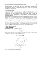
The saturation level can be observed in Fig. 9. In Fig. 10 have been plotted the air-gap flux
density, the 3-phase sinusoidal currents, axis torque and iron loss. It can be observed that the

air-gap flux-density value is very close to the one obtained from analytical approach, 0.826 T.
On the other hand, the rated torque is obtained based on rated current. Also, thanks to the
proper winding-slots-poles configurations, the torque ripples are significantly reduced. In fact,
the ratio of torque ripple is of 0.8% (maximum at 2.222 N
.
m and minimum at 2.204 N
.
m)! For
the computed iron loss (average value) a supplementary explanation is needed.
It has been observed that from analytical approach the iron loss is of 34.42 W. From FEM
analysis, the average value of iron loss is 27.573 W, meaning that an improved efficiency is
obtained. This difference can be explained regarding Fig. 9, where the flux density is
depicted in the machine’s active part. Here, the flux density varies significantly in the stator
iron, while in the analytical approach a fixed maximum flux density was used. Since the
FEM analysis has more credit, it can be said that 2% improved efficiency is obtained!
4. Optimization of the designed PMSM
After the design process and numerical validation, the optimization approach of the studied
electrical machine will be presented. Since we want to obtain a specific power for the
PMSM, we could say that our optimization objective will be to reduce the volume of the
machine (consequently the mass of the active parts of the machine), while the output power
is maintained constant (or very close to the desired value). Thus, the objective function is to
minimize the mass of the active parts of the PMSM. This mass, called
m
tot
is defined by the
mathematical expression:

totcopperrssspm
mm mmm=+++ (36)
where m

copper
refers to the mass of the winding copper, m
rs
is the mass of the rotor steel, m
ss

is the mass of the stator steel and m
pm
is the mass of the permanent magnet.
4.1 The optimization method
The optimization of studied electrical machine is based on gradient algorithm, (Tutelea &
Boldea, 2007). The main steps in the optimization algorithm are:
Step 1.
Choose the optimization variables (which will be modified in the process; starting
value and boundaries of the optimization variables are imposed).
Step 2.
Impose special limitations of other variables which can be altered during process.
Step 3.
Define the objective function.
Step 4.
Set initial and final value of global increment. The objective values will be initially
modified with larger increment, which will be further decreased in order to refine
the search space.
Step 5.
Compute geometrical dimensions, the electromagnetic parameters and the
characteristics (given in section 2.c), and evaluate the objective function.
Step 6.
Make a movement in the solution space and recompute the objective function and
its gradient. Use partial derivative to find the worse and the track points.
Step 7.

Move to the better solution, while the objective function is decreasing.
Step 8.
Reduce the variation step and repeat the previous steps. The algorithm stops when
the research movement cannot find better solution, even with smallest variation
step. The found value represents a local minimum; a different value can be found
by changing the initial starting point.

Electric Vehicles – Modelling and Simulations
192

Fig. 9. Flux-density and field lines for studied PMSM.
Color Shade Results
Quantity : |Flux density| Tesla

Time (s.) : 111.109999E-6 Pos (deg): 10.75
Scale / Color
27.0013E-9 / 139.34316E-3
139.34316E-3 / 278.68629E-3
278.68629E-3 / 418.02937E-3
418.02937E-3 / 557.37251E-3
557.37251E-3 / 696.71565E-3
696.71565E-3 / 836.0588E-3
836.0588E-3 / 975.40188E-3
975.40188E-3 / 1.11475
1.11475 / 1.25409
1.25409 / 1.39343
1.39343 / 1.53277
1.53277 / 1.67212
1.67212 / 1.81146
1.81146 / 1.9508

1.9508 / 2.09015
2.09015 / 2.22949
Global Design and Optimization of
a Permanent Magnet Synchronous Machine Used for Light Electric Vehicle
193

Fig. 10. FEM results of PMSM in motor regime.
The goal of the optimization process is to maximize the
power density (power/mass ratio) –
this is our objective function. The parameters to be varied, in the optimization process, are:
the length of the machine, the air-gap length, the PM length (on the magnetization
direction), the inner stator diameter, the stator slot’s height, the tooth width, the stator yoke
height and isthmus height. The initial values and the boundaries are given in Table 4.

parameter Initial value Boundaries
inner stator diameter (mm) 59 [30 …80]
slot height (mm) 13.4 [8 …18]
isthmus height (mm) 1.5 [0.7 …3]
height of the stator yoke 5 [3 …9]
width of stator tooth (mm) 4 [3 …8]
air-gap length (mm) 1 [0.5 …1.5]
height of the PM on magnetization direction (mm) 3 [2 …6]
length of the machine (mm) 43.5 [20 …60]
Table 4. Optimization variables: initial values and boundaries.
Supplementary constraints were considered for the mechanical outputs (torque and power)
and electrical (supplied current) characteristics, see Table 5.

parameter Bouderies
Axis torque (N
.

m) [2.1 … 2.3]
Output power (W) [340 … 360]
Supplied current (A) [13 … 18]
Table 5. Optimization variables: supplementary constraints.
0 5 10 15 20 25 30 35 40 45 50
-1
0
1
airgap lenght (mm)
airgap
flux-density (T)
0 0.001 0.002 0.003 0.004 0.005 0.006 0.007 0.008 0.009 0.01
-20
0
20
time (s)
3-phase
current (A)
0 0.001 0.002 0.003 0.004 0.005 0.006 0.007 0.008 0.009 0.01
2.1
2.2
time (s)
axis torque (N*m)
0 0.001 0.002 0.003 0.004 0.005 0.006 0.007 0.008 0.009 0.01
26
28
30
time (s)
iron losses (W)