Electric Vehicles Modelling and Simulations Part 15 pdf

Sugeno Inference Perturbation Analysis for Electric Aerial Vehicles

409

Fig. 8. UAV EPS Model at variable exogenous conditions with Sugeno (fuzzy-hybrid
system) and Sugeno parameter perturbations.
The inputs of Figure 5 are shown next in Figure 9 (top, centre graphs) while the resulting
thruster’s input electrical power is also shown (lower graph). The quasi-static approach
shows that the armature input electrical power does vary in order to balance the UAV flight
requirements for altitude and overcome the atmospheric air moisture conditions.
Clearly, Figure 10, shows a realisable UAV test scenario. Initially the UAV starts at ground (sea
level) and gradually gains altitude with a realisable climb rate. During its mission the UAV
remains at a fixed altitude and then gains altitude again reaching before its 6 km requirement,
where it remains for a given time (25 min) until it starts to descend back to sea level.
Meanwhile, the air moisture varies between two fuzzy logic extremes of “1” and “0.5” each
representing a different condition, “dry air” and “saturated moist air” respectively. The
moist air affects the temperature variation as the UAV altitude varies and hence was
modelled utilising the Sugeno FIS topology.
Based on the chapter hypothesis, the armature resistance will affect the propeller shaft
angular velocity for given conditions. Therefore, the next step is to observe the armature
resistance during the UAV mission and compare this to the nominal (sea level) conditions.
Figure 11, successfully demonstrates the nominal “blue line” armature resistance at sea level
and the variable resistance due to the altitude and air moisture conditions.
In Figure 11, the dotted upper and lower lines demonstrate the injected ±10% perturbation
in the Sugeno consequent. Both the effects of altitude, air moisture and the sensor SIEB type
of perturbations affect the thruster’s armature resistance and therefore it is expected to
observe this variation to cascade also to the thruster’s variables such as the propeller shaft
angular velocity.

Electric Vehicles – Modelling and Simulations

410
Figure 12, shows more clearly the injected ±10% perturbations in the Sugeno consequent
and the effect of these. Typically, the boundaries (upper and lower) indicate the line for
instantaneous measurements where the sensor measurement is used rather than the exact
value of the sensor.


Fig. 9. UAV thruster armature voltage, current and input electrical power.


Fig. 10. UAV operational scenario, indicating altitude and air moisture conditions.

Sugeno Inference Perturbation Analysis for Electric Aerial Vehicles

411

Fig. 11. Thruster armature resistance for nominal conditions (blue) and altitude based
conditions (red).
Normally, UAV propulsion pack designs have a limited maximum rated electrical power
which is available for use, including the propeller power requirements and thruster’s power
losses. Figure 12, shows the armature resistance related copper losses for the given UAV test
scenario. Clearly, the power copper losses relating to the nominal (sea level) when
compared to the variable altitude and air moisture conditions result in different losses. In
particular the variable altitude scenario power losses are less than the sea level equivalent,
hence resulting in a gain in net power available for thrust for the same power pack.


Fig. 12. Nominal (blue) and altitude based copper losses and propeller shaft powers.

Electric Vehicles – Modelling and Simulations

412
Figure 12, (lower graph), shows the propeller shaft available power for the test scenario
shown earlier. During time intervals (0,1500)s and (2200,3000)s the UAV requires its
maximum rated power in order to climb to the desired altitudes of 3000 m and 6000 m.


Fig. 13. Geared shaft RPM for nominal (blue) and altitude based (red), second graph
showing the percent variation in the shaft RPM.
Figure 13, shows (top graph) the propeller geared shaft RPM for the nominal (in blue) and
the altitude varied angular velocity (in red). As expected because the power pack has a
maximum rated power capability and the armature resistance losses reduce, the propeller
shaft mechanical power increases for the same rated input power. Hence, while the
propeller loading remains as shown in the previous profiles the angular velocity at the
propeller shaft is expected to increase as shown from the analysis.
Figure 13, also shows a zoomed version (lower graph) clearly showing the implications of
the added phenomenon of speed changing due to an example injected ±10% perturbations
in the Sugeno sensor. It appears that this specific injected perturbation does not cause a
substantial change compared to the altitude based angular velocities.
Figure 14. shows the armature resistance percentage error when compared to the sea level
conditions. Clearly the expected error (top graph) exceeds 20% from nominal, therefore
demonstrating the importance of the Sugeno fuzzy inference modelling within the context
of the fuzzy-hybrid modelling process. The armature resistance percentage error for both
the upper and lower boundaries (centre graph), are approximately 2.5 % for the
upper/lower boundary or 5% for both boundaries. This indicates that the Sugeno
perturbation based on SIEB-type errors can indeed affect the model behaviour. The (last
graph), shows the SIEB errors with reference to the sea level equivalent. These are expected
to be high and exceeding 20% due to the inclusion of the fuzzy-hybrid model which
includes the altitude/moisture and perturbation effects.

Figure 15 shows the thruster’s angular velocity error comparing the sea level and altitude
based models. Clearly the error (top graph) is nearly 5% and variant throughout the UAV
flight scenario. The centre graph shows the thruster’s upper and lower injected ±10%
perturbations in the Sugeno FIS and compared to the non-perturbation model. The error
resulting from this test run is less than 1%, thus shown some influence of the armature

Sugeno Inference Perturbation Analysis for Electric Aerial Vehicles

413
resistance variations cascading and affecting the propeller shaft angular velocity. However,
(last graph), when the perturbation model is compared to the sea level model the error
increased by approximately 10 times reaching a percentage error of up to 6%.


Fig. 14. Altitude-based armature resistance error with respect to the nominal (top graph);
altitude-based armature resistance error wrt ± 10% FIS Consequent perturbation (Centre
graph); the lower graph is showing the error due to ± 10% FIS Consequent perturbation wrt
the nominal armature resistance.


Fig. 15. Altitude-based shaft angular velocity error with respect to the nominal (top graph);
altitude-based angular velocity error wrt ± 10% FIS Consequent perturbation (Centre
graph); the lower graph is showing the error due to ± 10% FIS Consequent perturbation wrt
the nominal angular velocity.

Electric Vehicles – Modelling and Simulations

414
3. Conclusion
In this chapter we have learned how to incorporate sensor perturbations via the Sugeno

fuzzy logic inference for electrical thruster systems which are propelling a class of
electrically-powered unmanned aerial vehicles. Therefore, design considerations have
included the UAV altitude variation and atmospheric moisture via the fuzzy logic Sugeno
design framework.
Furthermore the necessity of the fuzzy-hybrid modelling topology became apparent for the
electrical thruster system. While the thruster was modelled utilising an ordinary differential
equation form, the additional UAV operational conditions such as altitude and atmospheric
moisture required the inclusion of the Sugeno-based fuzzy inference system thus
amalgamating the two topologies into a single fuzzy-hybrid topology.
4. Nomenclature
Nomenclature (Units are in SI)
n
Rule number
n
max

Maximum number of rules
j
Number of Sensors
j
max

Maximum number of sensors
z
j
j-th sensor variable
j
n
Z
Membership function for the

n
h
n-th rule function
123
(,,)
n
fzzz

Linear polynomial in terms of z
1
,z
2
, ,z
j

j
c
Centre for Gaussian type membership function for the j-th sensor
j
d
Dispersion for Gaussian type membership function for the j-sensor
η
Horizontal shift operator
n
b
Rule consequent offset
j
n

n-th rule j-th sensor polynomial coefficients

*
h
Sugeno FIS output at time

.
n


n-th rule rule firing
j


j-th sensor error
j

j-th sensor error upper boundary
j

j-th sensor error lower boundary
()
a
Vt
PMDC Armature thruster voltage
()t
Thruster angular velocity
()
a
it
Thruster Armature Current
a

K
Thruster back emf constant
a
R
Thruster armature resistance
a
R


Sugeno upper bound for armature resistance for different
altitudes

Sugeno Inference Perturbation Analysis for Electric Aerial Vehicles

415
a
R


Sugeno lower bound for armature resistance for different altitudes
L
Thruster inductance
a
E

Thruster equivalent back emf voltage
()t
Shaft angle
T
K

Thruster torque constant
m
T
Thruster produced torque
a
J

Thruster armature inertia
L
J
Load inertia
a
B

Thruster armature viscous angular damping
L
B
Load viscous angular damping
1
N

Thruster side gear teeth
2
N
Load side gear teeth
m
P

Thruster mechanical power


Constant in W
re
f
R

Reference resistance for thrusters armature at temperature
re
f
T
c
a
Coefficient of thermal expansion for copper


UAV Altitude in m

Air moisture condition
T

Temperature at altitude


re
f
T
Reference temperature
5. References
Kladis, G.P.; Economou, J.T.; Knowles, K.; Lauber, J. & Guerra T.M. (2010). Energy
conservation based fuzzy tracking for unmanned aerial vehicle missions under a priori

known wind information, Journal of Engineering Applications of Artificial
Intelligence, Vol. 24, Issue 2, pp. 278-294.
Karunarathne, L.; Economou J.T. & Knowles, K. (2007). Adaptive neuro fuzzy inference
system-based intelligent power management strategies for fuel cell/battery driven
unmanned aerial vehicles, Journal of Aerospace Engineering, Vol/ 224, No. G1, pp
77 – 88.
Sugeno, M. (1999). On stability of fuzzy systems expressed by fuzzy rules with singleton
consequents, IEEE Transactions on Fuzzy Systems, Vol. 7, Issue 2, pp 201-224.
Economou, J.T. & Colyer, R.E. (2005). Fuzzy-hybrid modelling of an Ackerman steered
electric vehicle, International Journal of Approximate Reasoning, Vol.41, No.3, pp.
343-368.
Ehsani, M.; Gao, Y.; Gay, S.E. & Emadi, A., (2005). Modern Electric, Hybrid Electric, and
Fuel Cell Vehicles, CRC Press, ISBN 0 8493 3154 4, USA.
Economou, J.T.; Tsourdos, A. & White B.A. (2007). Fuzzy logic consequent perturbation analysis
for electric vehicles , Journal of Automobile Engineering, Proceedings of the IMech E
PART D., Vol. 221, No D7, pp 757-765.

Electric Vehicles – Modelling and Simulations

416
Miller, J.M., (2004). Propulsion Systems for Hybrid Vehicles, IEE Power & Energy Series 45,
ISBN 0 86341 336 6, UK.
19
Extended Simulation of an Embedded
Brushless Motor Drive (BLMD) System for
Adjustable Speed Control Inclusive of a Novel
Impedance Angle Compensation Technique
for Improved Torque Control in
Electric Vehicle Propulsion Systems
Richard A. Guinee

Cork Institute of Technology
Ireland
1. Introduction
As already stated for the reasons given in a previous chapter a good continuous time
model, of low complexity, of a BLMD system is essential to adequately describe
mathematically the PWM inverter switching process with dead time and subsequent
binary waveform generation in terms of the switching instant occurrences for accurate
computer aided design (CAD) of embedded BLMD model simulation in proposed electric
vehicle (EV) propulsion systems. In this chapter a complete software model of the BLMD
system as a set of difference equations representing subsystem functionality, the
organization of these subsystem activities into flowchart form and the processing details
of these modular activities as software function calls in C-language for simulation
purposes (Guinee, 2003) is presented.
Furthermore in this the second chapter, concerning BLMD model fidelity for EV
applications, BLMD model simulation accuracy for embedded EV CAD is next checked for a
range of restraining shaft load torques via numerical simulation and then extensively
compared and benchmarked for accuracy against theoretical estimates using known
manufacturer’s catalogued specifications and motor drive constants (Guinee, 2003).
Model simulation accuracy is further substantiated and validated through evaluation of the
shaft velocity step response rise time when cross checked against (i) experimental test data
and (ii) that evaluated from the catalogued performance index relating to the brushless
motor dynamic factor (Guinee, 2003). Numerical simulation with outer velocity loop closure
is used to demonstrate the accuracy of the completed BLMD reference model, based on
established model confidence in torque control mode, in ASD configuration when compared
with experimental test data.
In addition to the BLMD model structure presented in the previous chapter for actual drive
emulation two innovative measures which relate to increased drive performance are also
provided. These novel techniques (Guinee, 2003), which include

Electric Vehicles – Modelling and Simulations

418
i. inverter dead time cancellation and
ii. motor stator winding impedance angle compensation,
are encapsulated within the BLMD model framework and simulated for validation purposes
and prediction of enhanced drive performance in EV systems. An approximate analysis is
given to support the approach taken and verify the performance outcome in each case.
In the first of these BLMD performance enhancements a novel compensation method has
already been presented in the first chapter to offset the torque reduction effects of inverter
delay during BLMD operation. This simple expedient relies on the zener diode clamping of
the triangular carrier voltage during the carrier waveform comparison with the modulating
current control signal in the comparator modulator to nullify power transistor turnon delay.
This approach obviates the need for separate compensation timing circuitry in each phase as
required in other schemes. The accuracy of this methodology is supported by current
feedback, EM torque generation and shaft velocity trace simulation when compared with
similar traces from the BLMD benchmark reference model with the effects of the inverter
basedrive trigger delay neglected.
The second proposed innovative improvement, presented in this chapter, relates to the
progressive introduction of commutation phase lead with increased shaft speed as BLMD
impedance angle compensation which forces the impedance angle to the same value as the
internal power factor angle. This effect maintains zero load angle between the stator
winding terminal voltage and the back emf. It also results in rated load torque delivery at
lower shaft speeds with minimal rise time, overshoot and settling time in the generated
torque for a range of torque demand input values. This novel technique greatly enhances the
dynamic performance of the embedded BLMD prime mover in EV applications without
overstressing mechanical assembly components during periods of rapid acceleration and
deceleration. The incorporation of this novel impedance angle compensation technique thus
minimizes component wear-out such as gear boxes, transmission shafts and wheel velocity
joints and consequently enhances overall EV reliability improvement. BLMD simulation is
provided in torque control mode at rated torque load conditions, for the actual drive system

represented, with and without impedance angle compensation to gauge model performance
accuracy over a range of torque demand step input values.
2. BLMD model structure and program sequence of activities
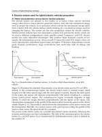
The BLMD model structure is composed of interconnected subsystems with feedback as
shown in Figure 1, of varying complexity according to physical principles. Consequently it can
be described by a discrete time configuration of first order digital filter realizations for linear
elements cascaded with difference equations representing nonlinear PWM inverter behaviour
into a complete software model for simulation purposes as illustrated in Figure 2. The BLMD
model program is organized into a sequence of software activities, coded in C-language as
function calls, representing the functionality of various subsystem modules shown as the
flowchart in Figure 3. All subsystem output (o/p) variable quantities in the cascaded activity
chain are assumed to remain constant, once computed irrespective of feedback linkage,
throughout the remainder of the time step interval t
k
based on the simulation sampling rates
(1/t
k
) chosen from considerations given in section 3.1 of the previous chapter. The essential
features of the BLMD model program in Figure 3 can be explained by means of the linked
modular software configuration encoded as the functional block sequence in Figure 2 along
with the appropriate C-language code segments illustrated in Figure 4.
Extended Simulation of an Embedded Brushless Motor Drive (BLMD) System for
Adjustable Speed Control Inclusive of a Novel Impedance Angle Compensation Technique

419
Pulse Width Modulator

-
+
Current


Filte r
H
DI
v
cj
3Current
Commutation
Filte r
H
T
Velocity Controller

G
V

Shaft Velocity
Filtering
I
dj
Position Resolver
RC De lay
v
lj=-Vs,
v
sj<0
,
v
sj0
1+sRC

1
=-V
s,
v
sj0
v
lj
,
v
sj0
1+sRC
1
Base Drive
v
bj
=V
B
,v
lj
V
th

=0 ,v
lj
V
th
V
th
V
th

v
lj
=V
B
,

=0 ,
v
lj
v
bj
v
bj
Inverter State Sj ( *)
S
j(0) {v
bj
=0,
S
j(1) {v
bj
>0,
S
j(2) {v
bj
=0,
>0}
=0}
=0}
v

bj
v
bj
v
bj
v
lj
v
lj
v
bj
v
bj
Tr i a ng ular
Carrier
Inverter Output
v
jg
=U
d
v
jg
=0
{
S
j
(1)
S
j
(2) & i

js
<0
S
j
(0)
S
j
(2) & i
js
>0
{
Stator Winding
Phase Voltage:
v
jg

v
js
+
Stator
Winding
Kt


l
+
Motor
Dynamics

e

-v
ej
Torque Constant
Bac k EMF Constant
Current Feedback

I
as
I
fj
+
-
Legend
Test Point
Phase j={a1,b2,c3}
V
tri
V
sj
=
V
s
, v
cj
 v
tri
-V
s
, v
cj

 v
tri



PWM
O/P
V
sj
V

r
K
c
1s

a
1s

b
Filter
H
FI
K
F
1  s

F
K
wi

Current
Demand
K
I
1s

d
sin p

r
 2( j 1)

3

1 s
Torque Demand
K
T
1s

T
K
p
 K
I
s

d
H
Vo


o
2
S
2


o
S 

o
2
V

V
js
 V
jg
 V
sg
V
sg

1
3
V
jg
j

1

r
s
sL
s
sin p

r
 2( j 1)

3


j
1
B
m
sJ
m
-
sin p

r
 2( j 1)

3


r

r

K
e
controller
G
I

Fig. 1. Transfer Function Block Diagram of a BLMD System (Guinee, 1999)

Electric Vehicles – Modelling and Simulations

420

Fig. 2-A. Software Functional Block Diagram (Guinee, 2003) of a BLMD System
Extended Simulation of an Embedded Brushless Motor Drive (BLMD) System for
Adjustable Speed Control Inclusive of a Novel Impedance Angle Compensation Technique

421

Fig. 2-B. Software Functional Block Diagram of a BLMD System

Electric Vehicles – Modelling and Simulations

422

Fig. 2-C. Software Functional Block Diagram of a BLMD System
Extended Simulation of an Embedded Brushless Motor Drive (BLMD) System for
Adjustable Speed Control Inclusive of a Novel Impedance Angle Compensation Technique

423

Fig. 3-A. Program Flow Diagram (Guinee, 2003) for BLMD Model Simulation
//Simul Time Step t
k-1
 t
k

For stepk = 0 to NDATA:
// Torque demand I/P:

k
d

Torq_dem = V
in

capture_filt_out ( );

I
nitializatio
setup_fo_filt ( );
init_vars ( );
run_to_pwmsw ( );
// Torque Demand Filtering
// i/ptorq_dem  
k
d
: o/pftorq_dem  
k

f

tdemf ( );
//Motor commutation
// i/pftorq_dem  
k
f
: o/ptor_sink[j]  
k
s

mot_commutator ( );
// Current Command Filtering

// i/p tor_sink[j]  
k
s
: o/pidemk[j]  i
k
d

idemf ( );
// Current Controller Operation
// i/p  {idek[j]-fifbk[j]}  {i
k
d
[j]- i
k
f
[j]}

//
o/p  vmpwmk[j]  v
k
c
[j]
cur_cont ( );
// Pulse Width Modulation
// i/p  {vmpwmk[j]-osc}  {v
k
c
[j]- v
k
tri
[j]}
//
o/p  vmpwmk[j]  v
k
c

pwm_mod ( );

test_pwm_xover (&pwm_sw_flag);
 Has PWM Com
p
arator O/P switched ? 
// Determine transition sw_time [j] = t
x
- t
k
via the

// regula falsi method over all three phases as

tt
X
tri k cj k
trik cjk trik cjk
vt vt t
vt vt vt vt
k






{( ) ( )}
{()()}{()()}
11
11
1


t
k
-1

t
k
t
x

cosc
v
k-1
tri

osc
v
k
tri
Time
Volta
g
e
cvmpwmk[j]
v
k-1
c

vmpwmk[j]
v
k
c

chord

t
j
sw_time[j] = t
x
Regula-Falsi Method

zeit =

t
sw_time[j] = t
j
max {t
j
}=t
m

t
*
inter_pwm_simulation (&pwm_sw_flag);
restore_filt_out ( );
// Redefine the simulation time step delt= t
j

// with carrier delay, t
d
= t
j
- t, in v
tri
(t - t
d
)
for (j=1;j ≤pwm_sw_flag;j++) {
delt = sw_time[j]; tdel = sw_time[j] - zeit;
if(j>1) delt = sw_time[j] - sw_time[j-1];
setup_fo_filt ( );

run_to_pwmsw ( );

run_post_pwmsw ( ); }
// Define the post PWM time step delt=t

- t
m
delt = zeit-sw_time[pwm_sw_flag]; tdel=0;
setup_fo_filt ( );
run_to_pwmsw ( );

run_post_pwmsw ( );
// Restore time step size
delt = zeit;
setup_fo_filt ( );

YES
NO
1
run_post_pwmsw ( );
// Capture all global variables subsequently
// affected by basedrive switching process
capture_drk_out ( );
//
R
un simulation of inverter basedrive delay
// turnon process affected by PWM
base_drive ( );
// Test for basedrive turnon { v
k

lj
[j]> v
th
}with
// complementary operation {
vj
lj
k
[]> v
th
}
test_drk_xover (&drk_sw_flag);
// Process basedrive switch transition flag
if (drk_sw_flag>0)
// interrogate basedrive turn ON and OFF
// times with subsequent inverter operation
inter_base_drk_sim (&drk_sw_flag);
else
// No basedrive switching - proceed with
// remaining BLMD model simulation
run_post_drksw ( );


Electric Vehicles – Modelling and Simulations

424


Fig. 3-B. Program Flow Diagram for BLMD Model Simulation
run_post_drk ( );

// Proceed with BLMD model subsystem
/
/

s
imulation a
f
te
r
basedrive activation
// Inverter O/P voltage generation
// i/p  Basedrive threshold voltages v
k
lj
[j]> v
th

// and
> v
th
and conduction states v
o

// o/pph_htk[j]  v
k
g
[j]
// Motor winding phase voltage generation
// o/pph_voltk[j]  v
k

s
[j]
pwm_inv ( );
// Motor winding simulation
// i/pph_voltk[j]  v
k
s
[j]
// o/pph_curk[j]  i
k
s
[j]: ifbk[j]  i
k
fc
[j]
winding ( );
// Current Feedback Filtering
// i/pifbk[j]  i
k
fc
[j]: o/pfifbk[j]  i
k
f
[j]
ifk ( );
// Electromagnetic Torque generation 
k
e
:
// i/pph_curk[j]  i

k
s
[j]: load_torq 
k
l
:
//
i/pcommutation psink[j]
// o/ptot_torq  
k
t
= (
k
e
-
k
l
)
convert_torqunit ( );
// Motor shaft velocity evaluation
// i/ptot_torq  
k
t
: o/pmot_shaft_vel  
k
m

// o/pelec_power  p
k
e

: mech_power  p
k
m
mot_shaft_velocity ( );
// Motor shaft position determination
// i/pmot_shaft_vel 
k
m
: o/pmot_shaft_pos 
k
m
mot_shaft_pos ( );
test_drk_xover (&drk_sw_flag);
 Is basedrive gating signal ON ? 
// Determine the switch times

t
x
j
= t
x
- t
k-1
via the
// piecewise linear approximation in (3.94) for
// basedrive gate signals
vj vj
lj
k
lj

k
and[] []
drk_sw_time[j] = t
x
j
; //max {t
x
j
}=t
m


t
k
-1
t
k
t
x
V
th
=0
Time

t
x
j
zeit =

t

Basedrive Voltage

t
**
1
inter_base_drk_sim (&drk_sw_flag);
restore_filt_out ( );
// Redefine the simulation time step delt= t
*
j

for (j=1;j ≤drk_sw_flag;j++) {
delt = drk_sw_time[j];
if(j>1) delt = drk_sw_time[j] - drk_sw_time[j-1];
setup_fo_filt ( );
base_drive ( );

run_post_drksw ( ); }
// Define time step after basedrive activation as
// delt=t
x
j
- t
m

delt = zeit-drk_sw_time[drw_sw_flag];
setup_fo_filt ( );
base_drive ( );

run_post_drksw ( );

// Restore time step size
delt = zeit;
setup_fo_filt ( );

YE
S
NO
Extended Simulation of an Embedded Brushless Motor Drive (BLMD) System for
Adjustable Speed Control Inclusive of a Novel Impedance Angle Compensation Technique

425
2.1 BLMD model simulation
Numerical simulation commences with the declaration of known BLMD system parameters
followed by a declaration with initialization of variables and three phase (3) arrays for
global usage, over the program linked function call sequence, as outlined in the code blocks
shown in Figure 4-1.


Fig. 4-1. Declaration and Initialization (Guinee, 2003)

Define BLMD System Parameters in Fig.5


// Define all filter constants:
K
T
=1.0;

T
=222S; // Torque Demand Filter H

T

K
I
=1.0;

I
=100S; // Current Demand Filter H
DI

K
F
=5.0;

I
=47S; //Current Feedback Filter H
FI
K
wi
 K
f
; // Current Feedback Factor

K
C
=19.5;

a
=225S;


b
=1.5mS; //Current Controller G
I

H
vo
=13.5x10
-3
; =√2; 
o
=2x10
3
rad.s
-1
; //Velocity Filter H
V

K
d
=1.0;

d
=28.6S; // RC Delay
r
S
=0.75; L
S
=1.94mH; p = 6 pole pairs; // Motor Winding
K
e

= K
t
=0.3 // Motor torque & Back EMF Constants
J
m
=3 kg.cm
2
; B
m
=2.14x10
-3
Nm.rad
-1
; // Motor Dynamics
U
d
=310 Volts; V
th
=0; V
S
=10 Volts; // Voltage Constants
f
S
=5.7kHz; A
d
=6.9 Volts; // Carrier Waveform Constants

Define Global Variables


stepk // k
th
iteration time step
delta_t // Fixed simulation Time Step Size t = (t
k
-t
k-1
)
delt // Variable simulation Time Step Size t
i

tdel // Carrier v
tri
(t-t
d
) time delay t
d

osc // Carrier amplitude v
k
tri

torq_dem // motor i/p torque demand 
k
d

ftorq_dem // Filtered torque demand 
k
f

mot_shaft_pos // Motor shaft position 
k
m

mot_shaft_vel // Motor shaft velocity 
k
m

tot_torq // Net drive torque 
k
f

 Define Global Array variables for j=1 to3 
ppsinkm1[j] // 3-phase commutation psink[j]
tor_sink[j] // 3-phase torque demand 
k
s
[j]
idemk[j] // 3-phase current demand i
k
d
[j]
fifbk[j] //Filtered current feedback i
k
f
[j]
ifbk[j] // Current feedback i
k
fc
[j]

vmpwmk[j] // Current controller o/p v
k
c
[j]
pwmtrk[j] // Modulator o/p v
k
sm
[j]
base_drk[j] // Basedrive o/p v
k
lj
[j]
bar_base_drk[j] // Complementary basedrive o/p vj
lj
k
[]
ph_voltk[j] // Stator winding Phase voltage v
k
s
[j]
back_emfk[j] // Motor back EMF v
k
e
[j]
ph_curk[j] // Stator winding Phase current i
k
s
[j]

init_vars ( )



// Function initializes all global variables and arrays to 0.0


Electric Vehicles – Modelling and Simulations

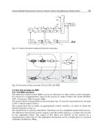
426

Fig. 5. Network Structure (Guinee, 1999) of a Typical Brushless Motor Drive System
Extended Simulation of an Embedded Brushless Motor Drive (BLMD) System for
Adjustable Speed Control Inclusive of a Novel Impedance Angle Compensation Technique

427
All first order linear system discretization is accomplished by complex variable substitution
of the Euler backward rectangular rule using the Z transform. The alternative filter
discretization process using Tustin’s bilinear method (Franklin et al, 1980) or the trapezoidal
integration rule (Balabanian, 1969) can also be used but with negligible observable
differences at the step size t chosen. Resultant digital filter implementation for simulation
purposes is facilitated by transfer of the appropriate filter time constant and gain coefficients
using the C-language ‘structure’ mechanism in the function call setup_fo_filt ( ) illustrated in
Figure 4-2.


Fig. 4-2. Linear Subsystem Discretization

setup_fo_filt ( )


// Function sets up and discretizes all first order BLMD

// linear subsystems H(s) in Figures 1 & 5 according
// to expressions (LX) and (LXIV) in the previous chapter as
Hs K k
c
s
s
sz
nnz
ddz
a
b
T
()
~( )









1
1
1
1
1
01
1

01
1



// using function call discrete1( );
// with discrete filter coefficients {k, n
0
, n
1
, d
0
, n
1
}, such as
tdemf( ); idemf( ); ifk( ); cur_cont( ); winding( );
mot_shaft_vel( ); mot_shaft_posn( );
dtrdfilt( ); // drive transistor RC delay network
typedef struct
{
double k;
double n0;
double n1;
double d0;
double d1;
} tf1;


First Order System Discretization Process discrete1 ( )


// Euler’s Backward Integration Rule
// sz
T
~( )
1
1
1 


double delt;
tf1 discrete1(tf1 temp)
{
tf1 discrete;
double at,bt,ts;
double k,n0,n1,d0,d1;
ts=delt; k=temp.k;
n0=temp.n0; n1=temp.n1;
d0=temp.d0; d1=temp.d1;
at=ts*n0; bt=ts*d0;
n0=at+n1; d0=bt+d1;
if(n1!=0.0) {
discrete.k=k*n1/d1;
discrete.n0=n0/n1;discrete.n1 = -1.0;
discrete.d0=d0/d1; discrete.d1 = -1.0;
} else {
discrete.k=k*n0/d1;
discrete.n0=1.0;
discrete.n1 = 0.0;
discrete.d0=d0/d1;
discrete.d1 = -1.0;

}
return discrete; }
// Tustin’s Bilinear Method
//
s
T
z
z
~
21
1
1
1





tf1 discrete1(tf1 temp)
{
tf1 discrete;
double at,bt,ts;
double k,n0,n1,d0,d1;
ts=delt;
bt=temp.d0*ts/2.0;
at=temp.n0*ts/2.0;
discrete.n0=at+temp.n1;
discrete.n1=at-temp.n1;
discrete.d0=bt+temp.d1;
discrete.d1=bt-temp.d1;

discrete.k=temp.k;
return discrete;}


Electric Vehicles – Modelling and Simulations

428
Before proceeding with model program execution in the k
th
time step (t
k-1
 t
k
) all global
variables and arrays are captured in the function call capture_filt_out ( ) for later
reinstatement, during accurate resolution of the width modulated pulse edge transition time
via the regula-falsi method, with restore_filt_out ( ) in Figure 4-3.


Fig. 4-3. Variable capture and restoration
The instruction code group run_to_pwmsw ( ) processes the sequence of BLMD software
activities up to the comparator modulator o/p using the following list of function calls in
Figures 4-1 and 4-4.
tdemf ( ) filters the i/p torque demand signal torq_dem with o/p ftorq_dem.
mot_commutator ( ) establishes the 3-phase reference psink[j], from the computed
shaft rotor displacement 
k
m
, for 3 phase stator winding voltage
commutation with modulated amplitude.

tor_sink[j] based on the filtered torque demand ftorq_dem.
idemf ( ) filters the i/p torque related current command signal tor_sink[j]
with o/p idemk[j].
cur_cont ( ) The lag compensator ‘optimizes’ the current error as the
difference between the current command idemk[j] and the filtered
stator winding current feedback fifbk[j] in each phase of the 3
current control loop. The o/p vmpwmk[j] from each of the high
gain controllers is amplitude limited to the saturation voltage
levels V
z
(~10v) by zener diodes.
pwm_mod ( ) produces a width modulated o/p pulse sequence pwmtrk[j] for
each phase in accordance with the amplitude comparison of the
modulating control signal vmpwmk[j] o/p and the triangular
dither signal osc. The modulator has a gain K
mod
with
complementary outputs, for basedrive operation, that are hard
limited to V
z
(~10v) by zener diodes.

capture_filt_out ( )


// Capture all global variables and arrays for PWM evaluation
void capture_filt_out(void)
{
int j;
cftorq_dem=ftorq_dem; cosc=osc;

ctot_torq=tot_torq; cmot_shaft_vel=mot_shaft_vel;
cmot_shaft_pos=mot_shaft_pos;
for(j=1;j<=3;j++) {
cidemk[j]=idemk[j]; ctor_sink[j]=tor_sink[j];
cvmpwmk[j]=vmpwmk[j]; cpwmtrk[j]=pwmtrk[j];}
return;}

restore_filt_out ( )


/ /Function reinstates arrays and global variables
ftorq_dem = cftorq_dem; //etc. for all other variables
for (j=1;j≤3; j++) {
idemk[j] = cidemk[j]; tor_sink[j]=ctor_sink[j];
vmpwmk[j]=cvmpwmk[j]; pwmtrk[j]=cpwmtrk[j];
}
Extended Simulation of an Embedded Brushless Motor Drive (BLMD) System for
Adjustable Speed Control Inclusive of a Novel Impedance Angle Compensation Technique

429

Fig. 4-4. Call Sequence to PWM O/P
A test is used to interrogate the o/p status of the simulated comparator modulator by
monitoring any observational sign change in the o/p polarity (±V
Z
), which is indicative of a
modulated pulse edge transition, after execution of the software code module pwm_mod ( )
as shown in Figure 4-5.

Fig. 4-5. Simulation of PWM
 run_to_pwmsw ( ) 
 tdemf ( ) 
// I/P Torque demand filtering
double torq_dem,td_km1;
double ftorq_dem,ftd_km1;
void tdemf(void)
{
ftd_km1= ftorq_dem;
ftorq_dem = fil_torq_sign*(dtdfilt.n0*torq_dem
+dtdfilt.n1*td_km1)*dtdfilt.k/dtdfilt.d0
-dtdfilt.d1*ftd_km1/dtdfilt.d0;
return; }
1
 mot_commutation ( ) 
// Three phase current commutation
double mot_shaft_pos; // Motor shaft position
void mot_commutator(void)
{
int j;
double temp1,temp2;
temp1=NPOLE*mot_shaft_pos;
temp2=2*PI/3;
ppsink[1]= cos(temp1);
ppsink[2]= cos(temp1-temp2);
ppsink[3] = -(ppsink[1]+ppsink[2]);
for(j=1;j<=3;j++) {tor_sinkm1[j]=tor_sink[j];
tor_sink[j]=ppsink[j]*ftorq_dem;}
return;}
2

 idemf ( ) 
// Current command filtering
void idemf(void)
{ int i;
for (i=1;i<=3;i++) {
idemkm1[i]=idemk[i];
idemk[i]=(didfilt.n0*tor_sink[i]
+didfilt.n1*tor_sinkm1[i])*didfilt.k/didfilt.d0
-didfilt.d1*idemkm1[i]/didfilt.d0; }
return;}
3
 cur_cont ( ) 
// BLMD Current controller simulation
double cont_errk;
void cur_cont(void)
{
int i;
double tempk,tempkm1;
cont_errk=0.0;
for(i=1;i<=3;i++) {
vmpwmkm1[i]=vmpwmk[i];
tempk=idemk[i]-fifbk[i];
tempkm1=cont_errk = idemkm1[i]-fifbkm1[i];
vmpwmk[i]= (dicont.n0*tempk
+dicont.n1*tempkm1)*dicont.k/dicont.d0
- dicont.d1*vmpwmkm1[i]/dicont.d0;
if(vmpwmk[i]>Vz+Vd) {vmpwmk[i]=Vz+Vd;
else
if(vmpwmk[i] < -(Vz+Vd)) {vmpwmk[i] = -
(Vz+Vd);}

return;}
4

pwm_mod ( )


// Pulse Width Modulator Function
double Vd=0.0; // RC shunt diode volt drop
double Vz=10.0; // Modulator saturation limits
double osc; // Carrier amplitude
void pwm_mod(void) {
double modop; // Modulator o/p
int j; osc=dither(); // Oscillator amplitude
for(j=1;j<=3;j++) {
modop = pwm_mod_sign*Kmod*(vmpwmk[j]- osc);
if(modop >= Vz+Vd) modop=Vz+Vd; else
if(modop <= -(Vz+Vd)) modop = -(Vz+Vd);
pwmtrkm1[j]=pwmtrk[j]; pwmtrk[j]=modop;}

5
 dither ( ) 
// PWM carrier waveform generation
double tdel, delta_t;
long stepk;
double dither(void) {
double pslp, period, temp;
period=1/Fd;
pslp=4*Ad*Fd; // slope of positive going ramp
temp=fmod(fabs(stepk*delta_t+tdel),period);
if(temp<period/2)

return (pslp*temp-Ad); // Pos. going ramp.
else
return (Ad-(temp-period/2)*pslp);}
//Neg. going ramp.
5A

Electric Vehicles – Modelling and Simulations

430
The o/p status of the comparator modulator is examined by comparing the trapped value
cpwmtrk[j] at the beginning of the time step t
k-1
with the new o/p pwmtrk[j] at t
k
for each phase
j and signalling any change via the pwm_test_flag in the function call test_pwm_xover ( ) detailed
in Figure 4-6. If a crossover event occurs during simulation then the transition interval t
X
=
(t
X
-t
k-1
), denoted by min-time, is determined by the regula falsi method in (LXVII) in the
previous chapter.


Fig. 4-6. Search for PWM X-over

test_pwm_xover (&pwm_test_flag)



// PWM Pulse Edge Transition Time Detection
void test_pwm_xover(int *flag)
{
int i, j, ref_sign, act_sign, sigfl;
double min_time, tol;
*flag=0;
// Reset pwm_sw_flag
tol=0.001;
// Tolerance limit on the time resolution
for(j=1;j<=3;j++) {
// Examine all 3  for PWM X-over
sigfl=0;
if(cpwmtrk[j]<0.0) ref_sign = -1; else ref_sign=1;
if(pwmtrk[j]<0.0) act_sign = -1; else act_sign=1;
if(ref_sign!=act_sign) {
// PWM Crossover Check
min_time=delt*(cosc-cvmpwmk[j])/(vmpwmk[j]
-cvmpwmk[j]-osc+cosc);
// Expression (3.85)
if(min_time<0.0)
nrerror("PWM Switch_time calculation error");
if(min_time<=(1-tol)*delt) {
// switch-time ≤ t = T
if(*flag>=1) {
for(i=1;i<=(*flag);i++)
if(min_time>=sw_time[i]-tol*delt &&
min_time<=sw_time[i]+tol*delt) sigfl=1;

// Switch times are identical - stall flag increase!
if(sigfl==0) { ++(*flag); phase_flag[*flag]=j;
sw_time[*flag]=min_time;} // Store switch time
} else { ++(*flag); phase_flag[*flag]=j;
sw_time[*flag]=min_time;}
}
// switch-time

t = T
} else ;
// No Crossover!
}
// End 3-phase X-over search!
if(*flag>0) {
// Adjust phase switching times

// in order of increasing magnitude
for(i=1;i<=(*flag);i++) { min_time=1.0;
for(j=i;j<=(*flag);j++) {
if(sw_time[j]<min_time) {
min_time=sw_time[j]; ref_sign=j;}
}
if(i!=ref_sign) {// Define swap (a,b,c): ca, ab, bc
SWAP(sw_time[i],sw_time[ref_sign],min_time);
SWAP(phase_flag[i],phase_flag[ref_sign],act_sign);}
}
}
return;}
Extended Simulation of an Embedded Brushless Motor Drive (BLMD) System for
Adjustable Speed Control Inclusive of a Novel Impedance Angle Compensation Technique

431
A check is made to see if this value occurs within the imposed tolerance limit (tol*delt) at the
end of the time step interval t
k
, denoted by delt, in which it is discarded in the affirmative
without test flag registration. If multiple crossover events occur within the simulation
interval, corresponding to different phases, then all transition times with the appropriate
phase tag number are logged in the respective sw_time[j] and test_flag[j] arrays along with
the signaled transition count via the PWM test flag. A check is also performed for identical
multiple switch transition times without an increase in test flag count. The test routine is
completed by arranging the multiple switch times, with corresponding phase listing, in
increasing order of magnitude for subsequent detailed PWM simulation in the function call
inter_pwm_simulation ( ). Accurate internal simulation of a modulated pulse transition,
indigenous to the time step, commences with restoration of the captured global variables
preceding the time step and temporary storage of the original step size (zeit) and time delay
(t_del) settings, relevant to the dither ( ) signal source, for later retrieval. The new time step
(delt) is initially set to the smallest switching interval t
1
X
(sw_time[1]) for discretization of all
first order linear subsystems using the call function setup_fo_filt ( ) as per the C-code module
in Figure 4-7.


Fig. 4-7. PWM X-Over Simulation
The necessary delay offset t
d
(tdel) is determined by back tracking (t
k

-t
1
X
) from t
k
for proper
time registration in the execution of the carrier function dither ( ) and rerun of the call sequence
run_to_pwmsw ( ) followed by the block function call run_post_pwmsw ( ). The post PWM

inter_pwm_simulation (&pwm_sw_flag)


//
Simulate 3

- PWM with accurate transition times t
X

void inter_pwm_simulation(int *flag)
{
int i,ref_sign,act_sign;
double zeit, t_del, tol=0.001;
zeit=delt; t_del=tdel; // Retain original time step info.
restore_filt_out();
for(i=1;i<=(*flag);i++) {
delt=sw_time[i]; // Adjust delt= (t
X
-t
k
) to X-over time t

X

if(i>1) delt -= sw_time[i-1];
tdel=t_del-zeit+sw_time[i];
setup_fo_filt();
run_to_pwmsw();
if(pwmtrk[phase_flag[i]]<0.0) act_sign = -1;
else act_sign=1;
if(cpwmtrk[phase_flag[i]]<0.0) ref_sign = -1;
else ref_sign=1;
if(ref_sign==act_sign) pwmtrk[phase_flag[i]] *= -1.0;
// Force PWM X-over
run_post_pwmsw();
} // adjust

t to complete interval (t
k
- t
X
)
delt=zeit-sw_time[*flag];
tdel=t_del; // Restore original timing to V
tri
(t)
setup_fo_filt();
run_to_pwmsw(); run_post_pwmsw();
delt=zeit; // Restore original time step
setup_fo_filt();
return;
}

Electric Vehicles – Modelling and Simulations

432
simulation call list contains the additional BLMD model basedrive switching features as an
embedded layer in the nested base_drive ( ) and associated switch event signalling
test_drk_xover ( ) program routines. The complete BLMD model program is subsequently
exercised for othermultiple switch time intervals t
i>1
x
with updated linear system
discretization and adjusted delay offset. Termination of the remainder of the original time step
simulation is accomplished by setting the integration interval delt equal to the time step
residue (t
k
-t
max
X
) followed by the call sequences run_to_pwmsw( ) and run_post_pwmsw ( )
and exiting to the main program with a reinstatement of original time settings
Numerical BLMD model simulation proceeds to the next program step in the flowchart
cycle shown in Figure 3, by processing the call sequence run_post_pwmsw ( ), with the
execution of the switch event routine base_drive ( ) associated with the basedrive turn-on/off
as a consequence of the PWM process. The relevant global variables and arrays associated
with this call sequence run are trapped by the command capture-drk_out ( ) as a precursor to
basedrive simulation. The ‘lockout’ circuit routine, illustrated in Figure 4-8, consists of the
integrating capacitor action when the PWM comparator o/p v
k
sm
[j] exceeds v

k-1
lj
[j] and
charge dumping when v
k
sm
[j] < v
k-1
lj
[j] as shown in Figure 3 for the basedrive BDJ with a
similar microprogram description for complementary basedrive
BDJ operation. The
exponential trigger voltage growth on the timing capacitor, due to the inherent RC circuit
delay in (LIV) in the previous chapter, along with the basedrive voltage threshold V
th
(0.0)
setting determines the inverter turn-on time. The charge dump action by the shunt diode
across the delay timing resistor is virtually instantaneous when the switched comparator
PWM output v
k
sm
[j]=K
mod
(v
k
c
[j]-v
k
tri
) is hard limited to -v

z
.


Fig. 4-8. Basedrive simulation
 run
_p
ost
_p
wmsw
(

)


 capture_drk_out( ) 
// Capture subsystem global variables and arrays
// pertaining to Basedrive switching evaluation
void capture_drk_out(void)
{
int j;
for(j=1;j<=3;j++) {
cbase_drk[j]=base_drk[j];
cbar_base_drk[j]=bar_base_drk[j];
cback_emfk[j]=back_emfk[j];
cph_curk[j]=ph_curk[j];
cph_voltk[j]=ph_voltk[j];
cifbk[j]=ifbk[j]; cfifbk[j]=fifbk[j];}
return;}
 base_drive ( ) 

//Simulation of Basedrive ‘lockout’ circuit with delay


void base_drive(void)
{
int j;
double barpwmtrk,barpwmtrkm1;
for(j=1;j<=3;j++) {
barpwmtrk = -pwmtrk[j]; barpwmtrkm1 = -pwmtrkm1[j];
base_drkm1[j]=base_drk[j];
bar_base_drkm1[j]=bar_base_drk[j];
if(DEL==1) { // Basedrive BDJ delay

activated
if(pwmtrk[j]>base_drkm1[j])//BDJ capacitor charge-up
base_drk[j]=(dtrdfilt.n0*pwmtrk[j]
+dtrdfilt.n1*pwmtrkm1[j])*dtrdfilt.k/dtrdfilt.d0
-dtrdfilt.d1*base_drkm1[j]/dtrdfilt.d0;
else
if(base_drkm1[j] >= (Vd+pwmtrk[j]))
base_drk[j]=pwmtrk[j]+Vd; //BDJ capacitor discharge
if(barpwmtrk>bar_base_drkm1[j]) // BDA operation
bar_base_drk[j]=(dtrdfilt.n0*barpwmtrk
+dtrdfilt.n1*barpwmtrkm1)*dtrdfilt.k/dtrdfilt.d0
-dtrdfilt.d1*bar_base_drkm1[j]/dtrdfilt.d0;
else if(bar_base_drkm1[j]>=(Vd+barpwmtrk))
bar_base_drk[j]=barpwmtrk+Vd;
} else if(DEL==0) { // BDJ delay switched OFF
base_drk[j]=pwmtrk[j];
bar_base_drk[j]=barpwmtrk;}

}
}
Extended Simulation of an Embedded Brushless Motor Drive (BLMD) System for
Adjustable Speed Control Inclusive of a Novel Impedance Angle Compensation Technique

433
This effect results in swift basedrive turn-off with zero delay when referenced to the trailing
edge of the PWM o/p. However the capacitor discharge can be gradual, when the PWM
o/p is soft switched (v
z
> v
k
sm
[j] > -v
z
), due to the limited magnitude of the product
combination of modulator gain K
osc
(~68) and error response v
k
c
[j] of the current loop
controller which is implicitly dependent on the filtered current feedback response i
k
f
[j] for
fixed current demand i
k
d
[j]. The gradual reduction in capacitor voltage protracts the

basedrive switch-off time, when referenced to the initial point of the logic “1-to-0”
transition, associated with the PWM trailing edge. This delay has to be accounted for in an
accurate inverter software model description with a search of the basedrive turn-off in
addition to the turn-on times associated with exponential voltage growth.
The BLMD program test function test_drk_xover (&drk_test_flag), which is shown in Figure
4-10 and is very similar to test_pwm_xover ( ) in code content, checks for basedrive on/off
firing signal occurrence within a simulation time step interval. This search is
complemented with the evaluation of associated multiple phase activation times t
i
x
for
both normal BDJ and complementary BDJ inverter drive modes of operation. These
inverter trigger instants t
i
x
are determined by piecewise linear approximation using
(LXXVI) in the previous chapter, ranked in increasing order of magnitude and phase
tagged via the global storage arrays drk_sw_time[j] and drk_phase_flag[j] for subsequent
use in detailed basedrive simulation. Accurate simulation of the basedrive trigger timing
signals for subsequent inverter operation is achieved using the software routine call
inter_base_drk_loop_sim (&drk_test_flag) which is shown in Figure 4-11 and has similar
execution features to inter_pwm_simulation ( ).
The function call begins with the reinstatement of the global arrays at the beginning (t
k-1
) of
the time step using restore_drk_out ( ), illustrated in Figure 4-9, and temporary storage (zeit)
of the original step size t. The routine proceeds with linear system discretization
appropriate to and with execution of the base_drive ( ) function and the subsequent call
sequence run_post_drksw ( ), listed in Figure 4-12, for progressive substitution of multiple
differential switch times as the temporary variable delt.

This simulation call is completed with restoration of the original time step size followed by
first order system discretization with a return to the main BLMD program to begin the new
time step t
k
 t
k+1
. The function call group run_post_drksw ( ), summoned during main
program execution in the flowchart of Figure 3, processes the following sequence of
modular software activities illustrated in Figures 4-12 and 4-13 pertaining to BLMD system
electrodynamic operation with inverter interaction.
pwm_inv ( ) generates the 3 inverter output HT binary voltage ph_htk[j]  v
k
g
[j] in response
to the PWM basedrive gating signals
bjbj
vv & shown in Figure 1. The magnitude of the
simulated complementary trigger signals
kk
&
ljlj
vv in relation to the basedrive BDJ threshold
voltage V
th
establish the conduction states }2,1,0{for )( kkS
J
as per (LV) in the previous
chapter, by means of the tristate switching indicator V
O
, of the complementary power

transistor pair T
J+
and T
J-
in each leg J of the 3 inverter shown in Figure 15 in the previous
chapter. The tristate flag condition in conjunction with the sustained stator winding current
flow ph_curk[j]  i
k
s
[j] through the free wheeling shunt diodes establish the inverter o/p
binary voltage as 0 or V
dc
. The neutral star point voltage Vng (v
sg
) of the stator winding is
determined from (LVIII) in the previous chapter for subsequent evaluation of the phase
voltages ph_voltk[j]  v
k
s
[j] via (LIX) in the previous chapter.