Electric Vehicles Modelling and Simulations Part 16 pot
Bạn đang xem bản rút gọn của tài liệu. Xem và tải ngay bản đầy đủ của tài liệu tại đây (1.14 MB, 28 trang )
Extended Simulation of an Embedded Brushless Motor Drive (BLMD) System for
Adjustable Speed Control Inclusive of a Novel Impedance Angle Compensation Technique
439
responsible for overshoot
ep
, accompanied by a corresponding reduction in settling time
as shown in Figure 11.
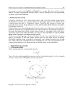
Fig. 10. Mutual Torque Characteristic Fig. 11. Torque Settling Time
3.1 Theoretical consideration of motor accelerative dynamical performance
The reduction in settling time is paralleled by the shaft velocity response time improvement
in reaching rated motor speed. It is evident from inspection of the velocity and torque
simulation traces that a direct correlation exists between the EM torque settling time and
motor shaft velocity response time as indicated in Table I.
Torque Load
l
=5Nm
“Inertial” Time Constant
m
=J
m
/ B
m
=0.318
Tran. Gain (Fi
g
.10)
K
=1.28
Torq-Dem
d
(Volts)
Av. Peak
EM Torq
ep
(Nm)
Torque
Overshoot
ep
-
l
(Nm)
Torq.
Settling
Time
T
setl
(sec)
Figs. 8/9
Shaft Velocity
Rise Time
T
res
(sec)
Figs. 6/7
Theoretical
Rise Time
T
r
(sec)
Eqn. (IV)
Rise Time
T
(sec) via
Dyn-Fac.
Eqn (VI)
5 6.2
1.2
~0.13
~0.13
0.131
0.107
6 7.45
2.45
~0.06
~0.06
0.057
0.0524
7 8.98
3.98
~0.04
~0.037
0.034
0.0323
8 10.29
5.29
~0.03
~0.027
0.025
0.0243
9 11.634
6.634
~0.024 ~0.022
0.02
0.02
Table I. Correlation of EM Torque Settling Time with Shaft Velocity Response Time
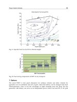
The shaft velocity step response rise time, as defined in Figure 6, can be obtained directly
from the solution of the transfer function (XCIX) from the previous chapter in the time
5 6 7 8
9
6
8
10
12
Torque Demand
d
Volts
E
M
T
o
r
q
u
e
Nm
Torque Mutual Characteristic
Average Peak EM Torque
ep
versus
Torque Demand
d
Simulated BLMD Mutual Torque Characteristic
e
p
Transfer Gain
K
=
ep
/
d
= 1.28
6 7.5 9 10.5 12
0.05
0.1
0.135
0.01
E
M Torque Step Respons
e
Settling Time T
setl
versus Peak EM Torque
ep
sec
T
setl
ep
Nm
Simulated EM Torque Step Response Settling Time
Electric Vehicles – Modelling and Simulations
440
domain with a step input approximation for the average peak torque overshoot
)(
lepep
in Figure 8 as
m
m
ep
t
B
r
et
/
1)(
(II)
with time constant
mmm
BJ
(III)
The step response time, for the shaft velocity under load conditions to reach maximum
speed
maxr
, can be determined from (II) for different torque demand i/p and
corresponding peak torque values as per the above Table I with
max
ln
rmep
ep
B
mr
T
(IV)
The estimated rise times are in excellent agreement with the approximate settling and
response times obtained from the BLMD model simulation traces. An alternative crude
estimate of the response time can be obtained from the motor “dynamic factor”
m
lep
r
Jdt
d
)(
(V)
for average peak torque endurance as the acceleration time
maxr
T
(VI)
from standstill to maximum speed assuming a shaft velocity linear transient response which
is valid for torque demand values in excess of 5 volts.
0 0.04 0.09 0.14 0.18
-40
-20
0
20
40
Motor Step Response with Load Torque
No Impedance Angle Compensation
Time (sec)
Motor Shaft Load
L
= 5Nm
Torque Demand
d
= 4v
Simulated Stator Back
Emf
v
ea
Simulated Impedance Voltage
V
Z
V
o
l
t
s
0.22 0.22 0.23 0.23 0.23
-200
-100
0
100
200
Motor Step Response with Load Torque
No Impedance Angle Compensation
Time (sec)
Motor Shaft Load
L
= 5Nm
Torque Demand
d
= 5v
Simulated Stator Back
Emf
v
ea
Simulated Impedance Voltage
V
Z
V
o
l
t
s
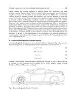
Fig. 12. Motor Winding Voltages Fig. 13. Motor Winding Voltages
Extended Simulation of an Embedded Brushless Motor Drive (BLMD) System for
Adjustable Speed Control Inclusive of a Novel Impedance Angle Compensation Technique
441
These response estimates, given in above Table I, are in good agreement with those already
obtained except for that at
d
= 5v where the rise time is longer with exponential speed
ramp-up.
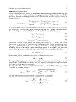
3.2 Torque demand BLMD model response - internal node simulation
The simulated back-EMF along with the stator impedance voltage drop are illustrated in
Figures 12 and 13 for two relatively close values of torque demand i/p. In the former case
the torque demand i/p of 4volts results in sufficient motor torque to meet the imposed shaft
load constraint (5Nm) without reaching rated speed and saturation (
10v) of the current
compensator o/p trace shown in Figure 14. The corresponding reaction EMF exceeds the
winding impedance voltage V
Z
and is almost in phase with the stator current, which is
proportional to V
Z
, at the particular low motor speed reached. The torque demand i/p of 5v
in the latter case results in the onset of a clipped current controller o/p in Figure 15 due to
saturation (
10) at rated motor speed
rmax
.
0 0.04
0.09
0.14
0.18
-5
0
5
Motor Step Response
No Impedance Angle Compensation
Time (sec)
Motor Shaft Load
L
= 5Nm
Torque Demand
d
= 4v
Simulated Current Compensator o/p
A
m
p
s
0.22
0.22 0.23 0.23
0.23
-10
0
10
18
-18
Motor Step Response
No Impedance Angle Compensation
Time (sec)
Motor Shaft Load
L
= 5Nm
Torque Demand
d
= 5v
Simulated Current Compensator o/p
A
m
p
s
Fig. 14. Current Compensator o/p Fig. 15. Current Compensator o/p
The back-EMF generated at this speed greatly exceeds the winding impedance voltage, as in
the former case, and leads the stator current necessary to surmount the torque load by the
internal power factor (PF) angle (~27
) with a correspondingly low power factor (~0.7).
The stator winding currents corresponding to the inputs
v9,v5
d
are displayed in
Figures 16 and 17 respectively which indicate the marked presence of peak clipping in the
latter case with loss of spectral purity due to heavy saturation of the current controller o/p
for
d
>5v.
The simulated motive power characteristic with the steady state threshold value of ~2.3kW
necessary to sustain shaft motion, for
d
=5v with restraining load torque and friction losses
is shown in Figure 18 at base speed
rmax
420 rad.sec
-1
.
Electric Vehicles – Modelling and Simulations
442
0 0.04 0.08 0.12 0.16
-12
-4
4
12
20
-20
Motor Step Response
No Impedance Angle Compensation
Time (sec)
Motor Shaft Load
L
= 5Nm
Torque Demand
d
= 5v
Simulated Motor Winding Current
i
as
A
m
p
s
i
as
0.08 0.084 0.088 0.092 0.096
-12
-4
4
12
20
-20
Motor Ste
p
Res
p
onse
No Impedance Angle Compensation
Time (sec)
Motor Shaft Load
L
= 5Nm
Torque Demand
d
= 9v
Simulated Motor Winding Current
i
as
A
m
p
s
i
as
Fig. 16. Stator Winding Current Fig. 17. Stator Winding Current
This can be rationalized from the power budget required to sustain the load torque at rated
speed via (LXXXVIII) in the previous chapter as
2.1kW)420)(5(
max
rll
P
(VII)
The excess coupling field power required to surmount mechanical shaft friction losses is
shown simulated in Figure 19 with a steady state estimate of ~200 watts.
0 0.06 0.12 0.18 0.24
750
1500
2250
3000
0
Motor Step Response
No Impedance Angle Compensation
Time (sec)
Motor Shaft Load
L
= 5Nm
Torque Demand
d
= 5v
Simulated Mechanical Power o/p
W
a
t
t
s
P
m
0 0.09 0.18 0.27 0.36
125
250
375
500
0
Motor Step Response
No Impedance Angle Compensation
Time (sec)
Motor Shaft Load
L
= 5Nm
Torque Demand
d
= 5v
Simulated Motive Power Equivalent
of Dynamic Friction
W
a
t
t
s
P
f
Dynamic Friction
P
f
=B
m
r
2
Fig. 18. Mechanical Power Delivery Fig. 19. Dynamic Friction Loss
Extended Simulation of an Embedded Brushless Motor Drive (BLMD) System for
Adjustable Speed Control Inclusive of a Novel Impedance Angle Compensation Technique
443
Stator Winding Phasor RMS Magnitude Estimation as per Figure 44 in previous chapter
via BLMD Model Simulation
Torq_Dem
d
Step i/p
Shaft_Vel
rmax
rad.sec
-1
Elec_Power P
e
volts (XLVII) –
Prev. Chap
Back_EMF
V
ej
volts
Imped_Vol
V
Z
volts
(XC) –
Previous Chap
Ph_Cur
I
js
amps
5v 419.2 2301 94.82 44.87 9.09
6v 420.3 2305 95.24 48 9.7
7v 418.9 2298 94.78 50.89 10.32
8v 410.3 2251 92.05 52.42 10.84
9v 405.5 2224 91.5 53.66 11.23
Derived Phase Quantities as per Figure 42 in previous chapter
Torq_Dem
d
volts
Int. PF Ang
I
(XCII) –
Prev. Chap.
I
Estimate
via
Figure 13
Ph_Vol
V
js
(XCIII) –
Prev. Chap
Imp_Ang
Z
(LXXXIV) –
Prev. Chap.
Load Ang
T
(XCV) –
Prev. Chap
PF Ang
I
+
T
5
27.13
27.13
126.44v
81.26 15.52 42.65
6
33.7
32.16
131.75v
81.28 15.6 49.3
7
38.43 38.74
136.56v
81.26 14.68 53.11
8
41.24
42.58
136.5v
81.08 13.83 55.07
9
43.8
45.12
138.1v
80.97 13.58 57.38
Table II. Phase Angle Evaluation for BLMD Steady State Operation with
l
= 5Nm
The effect of shaft load on the BLMD model simulation characteristics for
d
>5v is
summarized in above Table II for steady state conditions with the aid of the general phasor
diagram in Figure 42 of the previous chapter.
5 6 7 8 9
50
100
150
0
Motor Step Response
No Impedance Angle Compensation
Motor Shaft Load
L
= 5Nm
Motor Winding Phasor Voltages
V
o
l
t
s
Torque Demand
d
Volts
Impedance Voltage V
z
Back -
EMF
V
ej
Phase Voltage
V
js
5 6 7 8 9
20
40
60
0
M
otor Step Response
No Impedance Angle Compensation
Motor Shaft Load
l
= 5Nm
Motor Winding Phase Angles
V
o
l
t
s
Torque Demand
d
Volts
Load Angle
T
I
nternal Power Facto
r
A
ngle
I
P
ower Factor Angle
Fig. 20. Motor RMS Phasor Voltages Fig. 21. Stator Winding Phase Angles
Electric Vehicles – Modelling and Simulations
444
It is evident from the table that the back EMF has reached its peak rms value with the onset
of maximum shaft velocity, for all values of
d
>5V, with
V6.93)420(
2
315.0
2
maxmax
r
K
ej
e
V
(VIII)
Furthermore the impedance voltage drop V
z
in (XC) of the previous chapter is limited to a
very small increase with torque demand current I
dj
listed in Table II and is shown almost
stabilized to a constant value in Figure 20. This voltage clamping effect, due to current
compensator o/p saturation in response to tracking current feedback, is controlled to
achieve the desired rms level of clipped current flow in the stator winding as shown in
Figure 17 to satisfy torque load requirements. The rms winding current flow necessary at
unity internal power factor to meet steady state toque load and friction demands at ~5.4Nm
in Figures 8 and 9 can be determined from (XLV) in the previous chapter as
Amps 11.8
315.0
42.5
3
2
3
2
e
e
K
js
I
(IX)
This is almost identical to the rms values obtained from BLMD model simulations in Table
II, which are consistent with increased torque current demand, when internal power factor
self adjustments are accounted for as in
cos 8.1 Amps
js js I
II j=»
(X)
The internal power factor angles, listed in Table II and displayed in Figure 21, are deduced
for
d
>5v from the mechanical power transfer by substituting the rms quantities obtained
from back EMF and winding current simulations in expression (XCII) of the previous
chapter. These angles, which increase with torque demand i/p, can be alternatively
calculated from the simulated winding current response using (X) with knowledge of
js
I
.
The tabulated angle estimates obtained statistically as the phase lag between the current and
back EMF waveforms in Figure 13, for example, are in close agreement with those from
(XCII) of the previous chapter. The motor winding impedance angle
z
, which is fixed at
rated machine speed
rmax
, is determined from (LXXXIV) as ~81.2 in Table II.
The rms winding voltage V
js
is obtained in its pure spectral form, instead of the PWM
version furnished by the current controlled inverter, upon application of (XCIII) to the
known rms phasor quantities given in Table II for different values of
d
>5V.
Knowledge of the relevant phasor magnitudes with corresponding phase angles enable the
load angle
T
to be determined from (XCV) of the previous chapter for given shaft load
conditions. This is approximately fixed, at ~15
as indicated in Table II with about 2
variation, over the torque demand i/p range as shown in Figure 21. The resulting power
factor angle listed in Table II increases with
I
, for fixed load angle over the torque
demand i/p range as shown, in a way that is commensurate in (X) with motor current
requirements towards sustaining shaft load torque with a decreasing power factor as
illustrated in Figure 22.
Extended Simulation of an Embedded Brushless Motor Drive (BLMD) System for
Adjustable Speed Control Inclusive of a Novel Impedance Angle Compensation Technique
445
5 6 7 8 9
0.8
0.6
0.5
1
M
otor Step Response
No Impedance Angle Compensation
Motor Shaft Load
l
= 5Nm
Motor Power Factor Variation
Torque Demand
d
Volts
Fig. 22. Power Factor Variation
3.3 BLMD model simulation with novel impedance angle compensation
The effect of motor impedance angle compensation (MIAC), manifested as commutation
phase lead angle incorporated into the BLMD model in (XCVIII) of the last chapter as
33
2( 1) ( ) 2( 1)
rrz
pj p j
pp
qqj + on the motor step response velocity and torque
characteristics is illustrated in Figures 23 and 24 for the torque command i/p range
V9v4
d
at step size intervals of volt1
d
.
0 0.04 0.09 0.14 0.18
0
50
100
130
d
=7
d
=8
d
= 9
Motor Speed Characteristics
Rads.sec
-
1
Time (sec)
Motor Shaft Load
L
= 5Nm
S
h
a
f
t
S
p
e
e
d
Simulated Motor Shaft Velocity @
L
=5Nm
Motor Impedance Angle Compensation
(
MIAC
)
via
Commutation Phase Lead Angle
d
=6
d
=5
d
=5
0 0.007 0.01 0.02 0.03
0
5
10
d
=7
d
=8
d
= 9
Motor Torque Generation Characteristics
Time (sec)
Motor Shaft Load
L
= 5Nm
Simulated Motor Torque
e
@
L
=5Nm
Motor Impedance Angle Compensation
(
MIAC
)
via
Commutation Phase Lead Angle
d
=6
d
=5
d
=4
Nm
Fig. 23. Shaft Velocity with MIAC Fig. 24. Torque Response with MIAC
Electric Vehicles – Modelling and Simulations
446
The variation of peak torque overshoot with i/p demand, displayed as the mutual
characteristic in Figure 25, is linear with a transfer gain that is lower than that without MIAC
in Figure 10. Consequently the maximum peak torque delivery, for a given i/p demand to
sustain shaft load requirements, is lower in amplitude and of shorter overshoot pulse duration
as seen in Figure 24 when compared with that without MIAC in Figures 8 and 9. Furthermore
the persistence of torque overshoot is lower with a much reduced settling time (<0.015 sec), in
reaching steady state sustained load conditions in all cases albeit at lower acceleration and
much smaller drive speeds, thereby exerting less mechanical stress on the drive shaft
components and minimizing shaft flexure in EV propulsion applications.
4 5 6 7 8 9
6
7
8
9
10
5
ep
Nm
Torque Mutual Characteristic with TL
C
Peak EM Torque
ep
versus
Torque De mand
d
Transfer Gain
K
=
ep
/
d
= 1.2
Simulated BLMD Mutual Torque Characteristic
with Impedance Angle compensation
Torque Demand
d
Volts
4 5 6 7 8 9
40
60
80
100
120
20
Shaft Velocity
r
-
Torque
Demand
d
Transfer Characteristic
with
TLC
r
Rads.sec
-1
N
m
Simulated Velocity - Torque Dependency
with Impedance Angle Compensation
Transfer Coefficient
K
N
ri
di
i
N
1
1
12.05 rad.sec
-1
.Nm
-1
Torque Demand
d
Fig. 25. Mutual Torque with MIAC Fig. 26. Torque - Velocity Transfer Curve
4 5 8 9
20
60
80
-2
Impedance Angle Compensation
with
Commutation Phase Angle
Advance
D
e
g
r
e
e
s
Torque Demand
d
Commutation Phase Angle Lead Versus Torque Demand
r
Shaft Velocity
rad.sec
-1
Advance Angle
Degrees
54
23
Impedance Angle
Z
Internal PF Angle
I
PF Angle
Load Angle
T
54
112
365
4 5 6 7 8 9
0
20
40
60
Motor Ste
p
Res
p
onse
with Impedance Angle Compensation
Motor Shaft Load
L
= 5Nm
Motor Winding Phasor Voltages
V
o
l
t
s
Torque Demand
d
Volts
Impedance Voltage V
z
Back -
EMF
V
ej
Phase Voltage
V
js
Fig. 27. Impedance Angle Compensation Fig. 28. Phasor Voltages with MIAC
Extended Simulation of an Embedded Brushless Motor Drive (BLMD) System for
Adjustable Speed Control Inclusive of a Novel Impedance Angle Compensation Technique
447
The shaft velocity characteristics also indicate a much lower steady state motor run speed,
with MIAC deployed, which never reaches velocity saturation
-1
max
rads.sec 419
r
over the
permissible torque demand i/p range of
V.10V10
d
The relevant command torque to
shaft velocity transfer characteristic is approximately linear as shown in Figure 26 which
indicates a maximum motor operating speed of
-1
max
rad.sec 120
r
with
max
30%<
max
r
r
under rated load conditions (5Nm) for a maximum demand i/p of
dmax
=10V. This speed reduction is singly due to the maintenance of an almost zero load angle
T
shown in Figure 27, between the motor terminal V
js
and back EMF V
ej
rms voltage phasors
in Figure 45 of the previous chapter, by commutation phase angle advance for optimal
torque production as indicated from the BLMD simulation results in Table III.
This phase compensation technique results in back EMF and winding impedance voltage V
z
phasors that appear approximately equal in magnitude over the allowable torque demand
input range as shown in Figure 28. Furthermore the internal power factor angle
I
is forced
to adopt approximately the same value as the machine impedance angle
z
as indicated in
Table IIII, by the phase advance measure
z
in the current commutation circuit, with a
consequent collinear alignment of phasors V
ej
and V
z
in Figure 45. This collinear
arrangement can only be sustained at a particular machine speed that is dependent on the
torque demand i/p which determines the subsequent winding current flow and thus the
necessary impedance angle for alignment. This reasoning can be deduced as follows by
noting that for a given torque load
l
the rms winding current flow is linear with torque
demand i/p as per Table III and Figure 29.
Stator Winding Phasor RMS Magnitude Estimation as per Figure 45 of the Previous
Chapter via BLMD Model Simulation
Torq_Dem
d
Step i/p
Shaft_Vel
rmax
rad.sec
-1
Elec_Power P
e
(XLVII) in
Prev. Chap.
Back_EMF
V
ej
volts
Imped_Vol V
Z
volts – (XC) in
Prev. Chap.
Ph_Cur
I
js
amps
4v 18.6 94.44 4.17 6.06 7.76
5v 48.95 257.2 11.5 9.23 9.7
6v 70.87 363.67 16.01 13.05 11.71
7v 87.9 452.6 19.95 17.33 13.66
8v 102.9 531.2 23.28 22.18 15.7
9v 116.3 602.2 26.3 27.45 17.74
Derived Phase Quantities as per Figure 42 of the Previous Chapter
Torq_Dem
d
volts
Int. PF Ang
I
(XCII) in
Prev. Chap.
Ph_Vol V
js
(XCIII) in
Prev. Chap.
Imp_Ang
Z
(LXXXIV) in
Prev. Chap.
Load Ang
T
(XCV) in
Prev. Chap.
PFAng
I
+
T
4
13.75
10.23
16.1 1.39 15.14
5
36.13
20.73
37.22 0.51 36.64
6
49.71
29.06
47.72 -1.0 48.71
7
56.38
37.27
53.76 -1.22 55.16
8
61.02
45.44
57.95 -1.5 59.52
9
64.52
53.73
61.01 -1.79 62.73
Table III. Phase Angle Evaluation at
l
= 5Nm with Motor Impedance Angle Compensation
Electric Vehicles – Modelling and Simulations
448
4 5 6 7 8 9
10
15
20
5
I
js
Motor Step Response with Load Torque
Using Impedance Angle Compensation
Motor Shaft Load
L
= 5Nm
Simulated Motor Current
I
js
Variation
with Torque Demand i/p Voltage
d
A
m
p
s
Torque Demand
d
Volts
Motor Winding
Current
I
js
Fig. 29. Motor Current Variation
3.3.1 MIAC substantiation via theoretical analysis and validation
The internal power factor angle
I
can be determined theoretically for fixed winding current
flow corresponding to a given torque demand i/p using (IX) and (X), assuming negligible
dynamic friction at the shaft speeds concerned with
fl
, as
(
)
{
}
1
2
3
cos
l
tjs
I
KI
j
G
-
= (XI)
The motor terminal voltage i/p V
js
in (XCIII) from previous chapter can be optimized with
respect to the motor impedance angle
z
, which is unknown, in terms of the rms phasor
quantities V
ej
, V
z
and the fixed internal power angle
I
from (XI) by letting
()
0sin 0
js
z
dV
zI
dj
jj= - = (XII)
This procedure results in the impedance angle
z
in terms of the known angle
I
as
zI
jj= (XIII)
with
)(2
22
zejzejzejjs
VVVVVVVmax (XIV)
which is unknown as both V
ej
and V
z
depend on the motor shaft velocity
r
. The shaft
velocity can now be determined from (LXXXIV) from previous chapter using expression
(XIII) as
(
)
tan
s
s
r
rI
pL
wj= (XV)
Extended Simulation of an Embedded Brushless Motor Drive (BLMD) System for
Adjustable Speed Control Inclusive of a Novel Impedance Angle Compensation Technique
449
Theoretical Estimation of RMS Phasor Magnitudes
Torq_Dem
d
Step i/p
Ph_Cur
I
js
Table III
Int_PF
I
Eqn. (XI)
Shaft_Vel
r
Eqn (XV)
Back_EMF
V
ej
Eqn (VIII)
Imp_Vol
V
Z
Eqn. (XC) in
Prev. Chap.
Ph_Vol
V
js
Eqn. (XIV)
4v 7.76 A
15.37
17.71 rad/s 3.94v 6.04v 9.98v
5v 9.70 A
39.52
53.17 rad/s 11.84v 9.43v 21.27v
6v 11.71 A
50.28
77.55 rad/s 17.27v 13.74v 31.01v
7v 13.66 A
56.79
98.43 rad/s 21.92v 18.71v 40.63v
8v 15.70 A
61.54
118.87 rad/s
26.48v 24.71v 51.19v
9v 17.74 A
65.05
138.49 rad/s
30.85v 31.54v 62.39v
Table IV. Motor Impedance Angle Compensation
This value of
r
can be used to theoretically generate the rms voltage phasors V
ej
, V
z
and V
js
using expressions (VIII), (XC) and (XCIII) in the previous chapter respectively from a
knowledge of the motor winding phasor current
I
js
as per Table IV over the i/p torque
demand range range
V4
d
. The quantities obtained from BLMD simulations in Table III
compare reasonably well with those derived in Table IV from theoretical considerations
which reinforces model validation and confidence. The optimized internal power factor
angle, which is almost identical to that in Table III, results in a zero load angle
T
from
(XCV) in the previous chapter due to the phasor collinearity and thus improved torque
control via the PWM voltage supplied by the current controlled inverter. The power factor
angle , internal power factor angle
I
and machine impedance angle
z
variations with
torque demand i/p, which are displayed in Figure 27 using estimates extracted from BLMD
model simulation in Table III for
V4
d
, are almost congruent with a mismatched
difference manifested as the negligible load angle (
T
0).
4 5 6 7 8 9
0.8
0.6
0.4
0.3
1
IPF
I
mpedance Angle Compensation
with
Commutation Phase Angle
Advance
Torque Demand
d
Internal Power Factor (IPF) Variation with
Torque Demand
d
Internal Powe
r
Factor (IPF)
Volts
4 5 6 7 8 9
0.5
0.6
0.7
0.8
0.9
1
0.4
P
F
Motor Power Factor
(PF)
with Applied Shaft Load Torque
Motor Shaft Load
L
= 5Nm
Simulated Motor Power Factor Variation
with Torque Demand i/p Voltage
d
Torque Demand
d
Volts
Motor Power Factor with
Impedance Angle Compensation
Motor Power Factor without
Impedance Angle Compensation
Fig. 30. Motor Power Factor Fig. 31. Power Factor Comparison
Electric Vehicles – Modelling and Simulations
450
The internal power factor cos
I
j shows a gradual deterioration with increasing torque
demand i/p in Figure 30 as expected with the accompanying internal power factor angle
I
adjustment, from the mirrored motor current increase in Figure 29, constrained by a fixed
shaft load in (X). Impedance angle compensation results in a improved motor power factor
as shown in Figure 31 than that without MIAC over the torque demand i/p range
6VV4
d
necessary to meet load requirements
l
.
Motor speed reduction is also mirrored with a decrease of the shaft velocity step response
rise time as shown Figure 32 with maximum values falling below the velocity time response
floor of the uncompensated BLMD model. This results in constant motor speed operation,
though small by comparison to that without phase angle advance, well below the rated
value in torque control mode with smooth torque delivery to satisfy load requirements.
5
6
8 9
0.01
0.03
0.05
0.07
0.09
0.11
Nm
10%
90% Rise Time
t
r
of Shaft Velocity Step Response
with Motor Torque Loop Control
Motor Shaft Load
l
=5Nm
Zero MIAC
With MIAC
t
r
sec
Rise-times of Simulated Shaft Velocity Step Response
Torque Demand
d
Fig. 32. Shaft Velocity Rise Times
The simulated motor winding impedance and back EMF voltages for mid (5V) and full range
(9V) torque demand input values, which result in developed torque capable of surmounting
the fixed restraining shaft load (5Nm), are displayed in Figures 33 and 34. Both sets of
characteristics exhibit comparable amplitudes appropriate to the level of torque demand i/p,
with speed related motor current phase lags
I
as per Table III, that are much lower than those
without MIAC in Figure 13. The impedance and back EMF voltages are interrelated which can
be shown as follows by starting with expression (XC) for V
z
and using (IX) and (X) giving
(
)
(
)
2
3
cos
l
t
z
j
sI
K
VZI Z j
G
==
(XVI)
This can be rewritten by using (LXXXIV) in the previous chapter with optimized value of
I
in (XIII) as
Extended Simulation of an Embedded Brushless Motor Drive (BLMD) System for
Adjustable Speed Control Inclusive of a Novel Impedance Angle Compensation Technique
451
s
srs
t
l
r
Lpr
K
z
V
22
)(
3
2
(XVII)
0 0.03 0.05 0.08 0.1
-20
0
20
Motor Step Response with Load Torque
Using Impedance Angle Compensation
Time (sec)
Motor Shaft Load
L
= 5Nm
Torque Demand
d
= 5v
Simulated Stator Back
Emf
v
ea
Simulated Impedance Voltage
V
Z
V
o
l
t
s
0 0.03 0.06
-50
0
50
Motor Step Response with Load Torque
Impedance Angle Compensation Employed
Motor Shaft Load
L
= 5Nm
Torque Demand
d
= 9v
Simulated Stator Back
Emf
v
ea
Simulated Impedance Voltage
V
Z
V
o
l
t
s
Time (sec)
Fig. 33. Motor Winding Voltages Fig. 34. Motor Winding Voltages
The shaft velocity
r
, linking the back EMF, can be replaced in (XVII) by using (VIII)
yielding
]1[
2
21 ejz
VKKV (XVII)
where
612.5
3
2
1
t
l
K
s
rK (XVIII)
and
3
2
2
2
10855.4
st
s
rK
pL
K
(XIX)
from substitution of parameters in Table I of the previous chapter and
l
= 5Nm. The
impedance voltage in (XVII) is expressed as a quadratic equation in terms of the back EMF
with points of equality corresponding to
ejzej
VVV 29.79v v,915.6
(XX)
which are visible in Figure 28 as points of intersection of the two voltage traces.
Electric Vehicles – Modelling and Simulations
452
0 0.03 0.05 0.08 0.1
-16
-7
2
11
20
-25
t
Motor Step Response
Using Impedance Angle Compensation
Motor Shaft Load
L
= 5Nm
Torque Demand
d
= 5v
Simulated Motor Winding Current
i
as
A
m
p
s
i
as
0 0.03 0.05 0.08 0.1
-4
0
4
8
-8
Motor Step Response
With Impedance Angle Compensation
Time (sec)
Motor Shaft Load
L
= 5Nm
Torque Demand
d
= 5v
Simulated Current Feedback
i
fa
A
m
p
s
i
fa
Fig. 35. Stator Winding Current Flow Fig. 36. Motor Current Feedback
These crossover points divide the rms V
z
amplitude variation along with V
ej
in Figure 28
into three distinct regions, over the usable torque demand i/p range as per Table IV, with
29.8vfor
29.8v<6.9vfor
6.9vfor
ejejz
ejejz
ejejz
VVV
VVV
VVV
(XXI)
0 0.03 0.05 0.08 0.1
0
5
-5
Motor Step Response
With Impedance Angle Compensation
Time (sec)
Motor Shaft Load
L
= 5Nm
Torque Demand
d
= 5v
Simulated Current Compensator o/p
A
m
p
s
0 0.03 0.06
-40
-20-20
-20
0
20
35
Motor Step Response
Using Impedance Angle Compensation
Time (sec)
Motor Shaft Load
L
= 5Nm
Torque Demand
d
= 9v
Simulated Motor Winding Current
i
as
A
m
p
s
Fig. 37. Current Controller o/p Fig. 38. Stator Winding Current Flow
Extended Simulation of an Embedded Brushless Motor Drive (BLMD) System for
Adjustable Speed Control Inclusive of a Novel Impedance Angle Compensation Technique
453
These regions can also be inferred from the voltage amplitude traces in Figure 33 and 34
where V
ej
exceeds V
z
in the former case with v5
d
and vice versa for v9
d
in the latter
diagram.
0 0.03 0.06
-10
-5
0
-5
8
Motor Step Response
Impedance Angle Compensation Employed
Time (sec)
Motor Shaft Load
L
= 5Nm
Torque Demand
d
= 9v
Simulated Current Compensator o/p
A
m
p
s
0 0.01 0.03 0.04 0.06
-8
-1
6
13
-15
t
Motor Step Response
With Impedance Angle Compensation
Time (sec)
Motor Shaft Load
L
= 5Nm
Torque Demand
d
= 9v
Simulated Current Feedback
i
fa
A
m
p
s
i
fa
Fig. 39. Motor Current Feedback Fig. 40. Current Controller o/p
The simulated stator winding current along with current feedback response and current
controller o/p are displayed in Figures 35, 36 and 37 respectively for
v5
d
without
saturation related distortion in the current compensator o/p. The BLMD model simulation
current characteristics corresponding
v9
d
are also shown in Figures 38, 39 and 40
without saturation effects.
4. BLMD reference model simulation in velocity control mode
In this section the BLMD reference model performance as an ASD emulator is examined and
compared with experimental step response data for shaft inertial load conditions with
J
l
~
3
J
m
. Adjustable speed drive operation, with embedded inner PWM current control, is
effected by closing the outer velocity loop via a two term PI term controller
G
v
as shown in
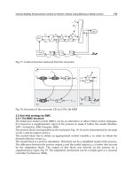
Figures 1 and 5. The analog velocity controller shown in Figure 41, which has an inbuilt
velocity offset adjustment and speed gain control adjustment
K
s
for the chosen BLMD
system modelled here (Moog GmbH, 1989) has a transfer function
s
K
pev
I
KKsG )( (XXII)
with proportional and integral compensation gain settings
K
p
and K
I
respectively. The
inclusion of this outer loop velocity compensator, in addition to the inner torque control
current loop, results in a complete holistic BLMD reference model that can now be used for
ASD simulation and performance evaluation in embedded applications. Proportional and
Electric Vehicles – Modelling and Simulations
454
integral control is easily incorporated in C-language routine during BLMD simulation of
velocity closed loop operation as a digital filter code module via (LXV) of the previous chapter
using the backward Euler method in (LXIV) of the previous chapter. The resulting ASD model
was exercised at low and high shaft velocities corresponding to 36.4% and 73.6% of rated
motor speed
n
o
in Table 1 of the previous chapter and compared with experimental test data at
critical internal nodes in Figure 1 for model validation and simulation accuracy.
+V
-V
Velocity Offset
A
djustment
K
P
K
I
s
Velocity Feedback
Velocity
Command
Input
V
r
Filtered Torque
Demand Input
Proportional
Control
Velocity
E
rro
r
Speed Gain
Adjustment
I
ntegra
l
Control
Controller Gain Settings
Proportional Gain K
P
=3.0
Integral Gain K
I
=233.5
Speed Gain K
s
=
0.824 <1.0
Velocity Offset = 0.017V
K
s
V
e
V
Fig. 41. BLMD Velocity Controller
The current controller
G
I
step response simulation traces for a velocity step command input
V
of 2volts, corresponding to 36% of rated motor speed (~4000rpm), are exhibited in
Figures 42 to 44 for linear pulsewidth modulator operation.
0 0.02 0.04 0.06 0.08 0.1 0.12 0.14 0.16 0.18 0.2
-6
-3
0
3
6
BLMD Benchmark Model Reference Simulation for Closed Loop Velocity Control Operation
Comparison of BLMD Current Demand Step Response Simulation with Experimental Test Data
for a 2 Volt Velocity Command Input
Current Demand
I
dj
(t)
(Amps)
Time (sec)
Medium Shaft Inertial Load Conditions:
J
mml
=12.3kg.cm
2
BLMD in Velocity Control mode with Step I/P Stimulus V
= 2 volt
Motor Current Optimizer: MCO-402B
Data Acquisition:
Sample Size
N
d
=5000; Sampling Rate
f
s
= 12.5kHz
BLMD Experimental Current Command Test Input
BLMD Reference Model Current Command Simulation
Simulation Time Step Size t =1s
Fig. 42. ASD Reference Model Current Demand Comparison with Experimental Test Data
Extended Simulation of an Embedded Brushless Motor Drive (BLMD) System for
Adjustable Speed Control Inclusive of a Novel Impedance Angle Compensation Technique
455
0 0.02 0.04 0.06 0.08 0.1 0.12 0.14 0.16 0.18 0.2
-6
-3
0
3
6
BLMD Benchmark Model Reference Simulation for Closed Loop Velocity Control Operation
Comparison of BLMD Filtered Current Feedback Step Response Simulation with Experimental Test Data
for a 2 Volt Velocity Command Input
Current feedback I
fj
(
t
)
(Amps)
Time (sec)
Medium Shaft Inertial Load Conditions: J
mml
=12.3kg.cm
2
BLMD in Velocity Control mode with Step I/P Stimulus
V
= 2 volt
Motor Current Optimizer:
MCO-402B
Data Acquisition:
Sample Size N
d
=5000; Sampling Rate f
s
= 12.5kHz
BLMD Experimental Current Feedback Test Response
BLMD Reference Model Current Feedback Simulation
Simulation Time Step Size
t =1
s
Fig. 43. ASD Model Reference Current Feedback Comparison with Experimental Test Data
0 0.02 0.04 0.06 0.08 0.1 0.12 0.14 0.16 0.18 0.2
-6
-3
0
3
6
BLMD Benchmark Model Reference Simulation for Closed Loop Velocity Control Operation
Comparison of BLMD Current Controller Step Response Simulation with Experimental Test Data
for a 2 Volt Velocity Command Input
Current Controller
Output
V
cj
(
t
)
(Volts)
Time (sec)
Medium Shaft Inertial Load Conditions: J
mml
=12.3kg.cm
2
BLMD in Velocity Control mode with Step I/P Stimulus
V
= 2 volt
Motor Current Optimizer:
MCO-402B
Data Acquisition:
Sample Size
N
d
=5000; Sampling Rate
f
s
= 12.5kHz
BLMD Current Controller Experimental Test Response
BLMD Reference Model Current Controller Output Simulation
Simulation Time Step Size
t =1
s
Fig. 44. ASD Model Current Controller o/p Comparison with Experimental Test Data
The accuracy of these simulation traces, which capture the essence of the velocity transient
step response V
r
overshoot in Figure 45, is characterized by a large waveform correlation
coefficient of fit in Table V which provides a good indication of the model fidelity when
matched with experimental data.
Electric Vehicles – Modelling and Simulations
456
0 0.02 0.04 0.06 0.08 0.1 0.12 0.14 0.16 0.18 0.2
-4
-3
-2
-1
0
1
BLMD Benchmark Model Reference Simulation for Closed Loop Velocity Control Operation
Comparison of BLMD Shaft Velocity Step Response Simulation with Experimental Test Data
for a 2 Volt Velocity Command Input
Shaft Velocity
V
r
(
t
)
(
Volts
)
Time (sec)
Medium Shaft Inertial Load Conditions:
J
mml
=12.3kg.cm
2
BLMD in Velocity Control mode with Step I/P Stimulus V
= 2 volt
Motor Current Optimizer:
MCO-402B
Data Acquisition:
Sample Size
N
d
=5000; Sampling Rate
f
s
= 12.5kHz
BLMD Ex
p
erimental Shaft Velocit
y
Test Res
p
onse
BLMD Reference Model Shaft Velocity Simulation
Simulation Time Step Size
t =1
s
Velocity Command Setting
-V
= 2Volts
Fig. 45. ASD Model Reference Shaft Velocity Comparison with Experimental Test Data
Target Data Length
N
D
=3000
Data Sampling Rate:
12.5kHz
BLMD Simulation
Time Step: 1
s
Waveform Correlation Analysis for Total Inertial Shaft Load
J
Tot
= J
l
+ J
m
. =12.3kg.cm
2
ASD Waveform
Velocity Command i/p
V
= 2V
Velocity Command i/p
V
= 4V
Current Demand I
d
j
96.8% 92.85%
Current Feedback (FC) I
fj
97.26% 93.27%
Current Compensator output V
c
j
59.81% 45.46%
Motor Shaft Velocity output V
r
99.8% 99.68%
Table V. ASD Model Trace Simulation Comparison with Experimental Test Data
The simulated current demand and feedback waveforms, which have high matching
coefficients with test data, exhibit an amplitude modulated step response with velocity
transient overshoot and ringing, before eventually setting to negligible constant amplitude
traces with fixed frequency commensurate with reached shaft speed
r
demanded (V
r
~2V)
in Figure 45.
The compensated velocity error output for 2Volts operation V
r
in the BLMD network
structure in Figure 5 is equivalent to the filtered torque demand
df
, as the velocity control
effort
V
e
shown in Figure 46, applied to the inner closed loop for motor current control and
BLMD output torque regulation. This optimized velocity error
V
e
in Figure 46 is a short
duration pulse for reasons of fast BLMD shaft velocity risetime
T
res
and short setting time
T
setl
as required in high performance ASD industrial applications.
Extended Simulation of an Embedded Brushless Motor Drive (BLMD) System for
Adjustable Speed Control Inclusive of a Novel Impedance Angle Compensation Technique
457
0 0.03 0.06 0.09 0.12 0.15 0.18 0.21 0.24
-4
0
4
8
BLMD Benchmark Model Reference Simulation for Closed Loop Velocity Control Operation
Velocity Controller Error Output Simulation for a 2 Volt Velocity Command Step Input
Velocity Controller
Output (Volts)
Time (sec)
Medium Shaft Inertial Load Conditions:
J
mml
=12.3kg.cm
2
BLMD in Velocity Control mode with Step I/P Stimulus
V
= 2 volt
Motor Current Optimizer:
MCO-402B
BLMD Reference Model Velocity Controller Output Simulation
Simulation Time Step Size
t =1
s
Xovr
Fig. 46. ASD Reference Model Compensated Velocity Error Output
The presence of overshoot in the BLMD velocity step response in Figure 45 is due to the
non-optimal tuning of the velocity controller PI parameters required to ensure stiff
dynamical operation for the total drive shaft inertial load
J
Tot
= J
m
+J
l
in question.
0 0.04 0.08 0.12 0.16 0.2 0.24 0.28 0.32
-3
-2
-1
0
BLMD Benchmark Model Reference Simulation for Closed Loop Velocity Control Operation
ASD Shaft Velocity Output Simulation V
r
for a Velocity Command Step Input V
= 2 Volt
at Various Shaft Inertial Loads
J
Tot
Shaft Velocity O/P
V
r
(Volts)
Medium Shaft Inertial Load Conditions:
J
mml
= 12.3kg.cm
2
ASD Rotor Inertia:
J
m
= 3.04kg.cm
2
Motor Current Optimizer:
MCO – 402B
Simulation Time Step Size:
t=1
s
BLMD Reference Model Shaft Velocity Step Response for
Various Inertial Loads
J
Tot
J
Tot
=8
J
m
_______
J
Tot
=6
J
m
_______
J
Tot
=4
J
m
_______
J
Tot
=3
J
m
_ _ _ _ _
J
Tot
=2
J
m
_ _ _ _ _
J
Tot
=
J
m
_ _ _ _ _
Time (sec)
Overshoot
V
r
= V
r
(t
p
) - V
r
(t
)
t
p
Fig. 47. ASD Shaft Velocity Step Response Variation with Rotor Inertial Load
J
Tot
Electric Vehicles – Modelling and Simulations
458
0 0.04
0.08 0.12 0.16 0.2 0.24 0.28 0.32
-4
0
4
8
12
BLMD Benchmark Reference Model Simulation for Closed Loop Velocity Control Operation
ASD Velocity Controller Error Output Simulation for a 2 Volt Velocity Command Step Input
at Various Shaft Inertial Loads
J
Tot
Shaft Controller O/P
V
e
(Volts)
Medium Shaft Inertial Load Conditions:
J
mml
= 12.3kg.c
m
2
ASD Rotor Inertia:
J
m
= 3.04kg.cm
2
Motor Current Optimizer:
MCO – 402B
Simulation Time Step Size:
t =1
s
BLMD Reference Model Shaft Velocity Step Response for
Various Inertial Loads
J
Tot
J
Tot
=8
J
m
_______
J
Tot
=6
J
m
_______
J
Tot
=4
J
m
_______
J
Tot
=3
J
m
_ _ _ _ _
J
Tot
=2
J
m
_ _ _ _ _
J
Tot
=
J
m
_ _ _ _ _
Time (sec)
Fig. 48. Variation of ASD Velocity Control Effort with Rotor Inertial Load
J
Tot
0 1 2 3 4 5 6 7 8
9
0
50
100
150
200
250
300
Motor Shaft Load
J
l
– Multiples of Rotor Inertia
J
m
ASD Settling Time
T
setl
(ms)
ASD Shaft Velocity Step Response Settling Time
T
setl
Variation with
Rotor Shaft Inertial Loading for Different Command Velocities
ASD Rotor Inertia:
J
m
= 3.04kg.cm
2
Motor Current Optimizer:
MCO – 402B
ASD
Simulation Time Step Size:
t =1
s
ASD Velocity Demand
V
= 2Volts
______
ASD Velocity Demand
V
= 4Volts
______
Fig. 49. Variation of ASD Settling Time with Inertial Loading
Extended Simulation of an Embedded Brushless Motor Drive (BLMD) System for
Adjustable Speed Control Inclusive of a Novel Impedance Angle Compensation Technique
459
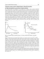
Examination of the ASD velocity step response trace simulations over a range of shaft
inertial load multiples of the rotor value
J
m
in Figure 47 reveal that the PI parameters have
been optimized only at zero load with
J
Tot
= J
m
for good drive dynamic transient
performance with little overshoot. The effect of increased shaft inertia on the velocity control
effort
V
e
in Figure 48, for a velocity command input of 2 volts, is a greater sustained
oscillation accompanied by longer settling times
T
setl
manifested in the simulated ASD
velocity step response as shown in Figure 49. This behaviour is mirrored by an increased
overshoot, as defined in Figure 47, in the BLMD shaft velocity step response with shaft load
inertia as shown in Figure 50.
The effect of increased load inertia on ASD dynamic performance also translates into slower
rise times
T
res
as shown in Figure 51 for a non optimally tuned velocity controller.
Further ASD step response simulation and comparison with experimental measurements in
Figures 52 to 55, for a 4 volts velocity command input which corresponds to 74% of rated
motor speed
n
0
with resulting saturated pulsewidth modulator operation in Figure 54 for the
load inertia considered (~12.3kg.cm
2
), reveal good BLMD model accuracy.
0 1 2 3 4 5 6 7 8 9
10
18
26
34
42
50
Motor Shaft Load
J
l
– Multiples of Rotor Inertia
J
m
ASD % Overshoot (
V
r
/
V
r
)100%
ASD Shaft Velocity Step Response Percentage Overshoot Variation with
Rotor Shaft Inertial Loading for Different Command Velocities
ASD Rotor Inertia:
J
m
= 3.04kg.c
m
2
Motor Current Optimizer:
MCO – 402B
ASD
Simulation Time Step Size:
t =1
s
ASD Velocity Demand
V
= 2Volts
______
ASD Velocity Demand
V
= 4Volts
______
Fig. 50. Variation of ASD Shaft Velocity Overshoot with Inertial Loading
Electric Vehicles – Modelling and Simulations
460
0 1 2 3 4 5 6 7 8 9
10
20
30
40
50
60
Motor Shaft Load
J
l
– Multiples of Rotor Inertia
J
m
ASD Rise Time
T
res
(ms)
ASD Shaft Velocity Step Response Rise Time T
res
Variation with
Rotor Shaft Inertial Loading for Different Command Velocities
ASD Rotor Inertia:
J
m
= 3.04kg.c
m
2
Motor Current Optimizer:
MCO – 402B
ASD Simulation Time Step Size:
t =1
s
ASD Velocity Demand
V
= 2Volts
______
ASD Velocity Demand
V
= 4Volts
______
Fig. 51. Variation of ASD Velocity Response Rise Time with Load Inertia
0
0.02 0.04 0.06 0.08 0.1 0.12 0.14 0.16 0.18 0.2
-12
-8
-4
0
4
8
12
BLMD Benchmark Model Reference Simulation for Closed Loop Velocity Control Operation
Comparison of BLMD Current Demand Step Response Simulation with Experimental Test Data
for a 4 Volt Velocity Command Input
Current Demand
I
dj
(t)
(Amps)
Time (sec)
Medium Shaft Inertial Load Conditions: J
mml
=12.3kg.cm
2
BLMD in Velocity Control mode with Step I/P Stimulus V
= 4 volt
Motor Current Optimizer: MCO-402B
Data Acquisition:
Sample Size N
d
=5000; Sampling Rate f
s
= 12.5kHz
BLMD Experimental Current Command Test Input
BLMD Reference Model Current Command Simulation
Simulation Time Step Size t =1s
Fig. 52. BLMD Reference Model Current Demand Comparison with Experimental Test Data
Extended Simulation of an Embedded Brushless Motor Drive (BLMD) System for
Adjustable Speed Control Inclusive of a Novel Impedance Angle Compensation Technique
461
0 0.02 0.04 0.06 0.08 0.1 0.12 0.14 0.16 0.18 0.2
-12
-8
-4
0
4
8
12
BLMD Benchmark Model Reference Simulation for Closed Loop Velocity Control Operation
Comparison of BLMD Filtered Current Feedback Step Response Simulation with Experimental Test Data
for a 4 Volt Velocity Command Input
Current feedback I
fj
(
t
)
(Amps)
Time (sec)
Medium Shaft Inertial Load Conditions:
J
mml
=12.3kg.cm
2
BLMD in Velocity Control mode with Step I/P Stimulus
V
= 4 volt
Motor Current Optimizer:
MCO-402B
Data Acquisition:
Sample Size
N
d
=5000; Sampling Rate
f
s
= 12.5kHz
BLMD Experimental Current Feedback Test Response
BLMD Reference Model Current Feedback Simulation
Simulation Time Step Size t =1s
Fig. 53. BLMD Model Current Feedback Comparison with Experimental Test Data
0 0.02 0.04 0.06 0.08 0.1 0.12 0.14 0.16 0.18 0.2
-12
-8
-4
0
4
8
12
BLMD Benchmark Model Reference Simulation for Closed Loop Velocity Control Operation
Comparison of BLMD Current Controller Step Response Simulation with Experimental Test Data
for a 4 Volt Velocity Command Input
Current Controller
Output V
cj
(
t
)
(Volts)
Time (sec)
Medium Shaft Inertial Load Conditions: J
mml
=12.3kg.cm
2
BLMD in Velocity Control mode with Step I/P Stimulus
V
= 4 volt
Motor Current Optimizer: MCO-402B
Data Acquisition:
Sample Size N
d
=5000; Sampling Rate f
s
= 12.5kHz
BLMD Current Controller Experimental Test Response
BLMD Reference Model Current Controller Output Simulation
Simulation Time Step Size
t =1
s
Fig. 54. BLMD Model Current Controller Output Comparison with Experimental Test Data
Electric Vehicles – Modelling and Simulations
462
0 0.02 0.04 0.06 0.08 0.1 0.12 0.14 0.16 0.18 0.2
-8
-6
-4
-2
0
2
BLMD Benchmark Model Reference Simulation for Closed Loop Velocity Control Operation
Comparison of BLMD Shaft Velocity Step Response Simulation with Experimental Test Data
for a 4 Volt Velocity Command Input
Shaft Velocity
V
r
(
t
)
(Volts)
Time (sec)
Medium Shaft Inertial Load Conditions:
J
mml
=12.3kg.cm
2
BLMD in Velocity Control mode with Step I/P Stimulus V
= 4 volt
Motor Current Optimizer: MCO-402B
Data Acquisition:
Sample Size N
d
=5000; Sampling Rate f
s
= 12.5kHz
BLMD Experimental Shaft Velocity Test Response
BLMD Reference Model Shaft Velocity Simulation
Simulation Time Step Size
t =1
s
Velocity Command Setting
-V
= 4Volts
Fig. 55. BLMD Model Shaft Velocity Comparison with Experimental Test Data
The quality of ASD simulation trace match with test data is indicated by the high value of
the waveform correlation coefficients given in Table V.
0 0.03 0.06 0.09 0.12 0.15 0.18 0.21 0.24
-4
0
4
8
12
16
B
LMD Benchmark Model Re
f
erence Simulation
f
or Closed Loop Velocit
y
Control Operation
Velocity Controller Error Output Simulation for a 4 Volt Velocity Command Step Input
Velocity Controller
Output (Volts)
Time (sec)
Medium Shaft Inertial Load Conditions: J
mml
=12.3kg.cm
2
BLMD in Velocity Control mode with Step I/P Stimulus
V
= 4 volt
Motor Current Optimizer:
M
CO-402B
BLMD Reference Model Velocity Controller Output Simulation
Simulation Time Step Size
t =1
s
X
ovr
Velocity Error Saturation
V
Z
=
10V
Pulse Duration
*
Fig. 56. BLMD Reference Model Compensated Velocity Error Output
Extended Simulation of an Embedded Brushless Motor Drive (BLMD) System for
Adjustable Speed Control Inclusive of a Novel Impedance Angle Compensation Technique
463
The velocity loop derived torque command input stimulus V
e
in Figure 56 has a pulse
duration that is much shorter than the time constant (
ml
~ J
tot
/B
m
) of the load dynamics,
eventhough the pulse amplitude is of sufficient strength to force the shaft velocity to the
value demanded (
V
~4volts). The endurance
*
of the velocity control effort in Figure 56,
associated with pronounced PWM saturation in Figure 54, is a measure of the maximum
sustained EM torque necessary to accelerate the total BLMD inertial load masses to the
appropriate shaft velocity demanded by the ASD command setting
V
. This velocity error
pulse has amplitude that is clipped to a maximum saturation limit of 10 volts at the three
phase current generator input, which limits the size of the torque loop input stimulus, in the
derivation of the BLMD current command signals.
Examination of the family of characteristics pertaining to velocity control effort over a range
of motor shaft inertial loads in Figure 57 indicate peak saturation over long pulse intervals
*
proportional to the inertial masses as in Figure 58
to be accelerated to the required speed
V
r
. This velocity error saturation is absent in the characteristics displayed in Figure 48 for
2volt ASD operation and results in linear PWM operation with a BLMD acceleration torque
delivery commensurate with the velocity effort.
0 0.04 0.08 0.12 0.16 0.2 0.24 0.28 0.32
-4
0
4
8
12
BLMD Benchmark Reference Model Simulation for Closed Loop Velocity Control Operation
ASD Velocity Controller Error Output Simulation for a 4 Volt Velocity Command Step Input
at Various Shaft Inertial Loads
J
Tot
Shaft Controller O/P
V
e
(Volts)
Medium Shaft Inertial Load Conditions:
J
mml
= 12.3kg.c
m
2
ASD Rotor Inertia:
J
m
= 3.04kg.cm
2
Motor Current Optimizer:
MCO – 402B
Simulation Time Step Size:
t =1
s
BLMD Reference Model Shaft Velocity Step Response for
Various Inertial Loads
J
Tot
J
Tot
=8
J
m
_______
J
Tot
=7
J
m
_______
J
Tot
=6
J
m
_______
J
Tot
=5
J
m
_______
J
Tot
=4
J
m
_ _ _ _ _
J
Tot
=3
J
m
_ _ _ _ _
J
Tot
=2
J
m
_ _ _ _ _
J
Tot
=
J
m
_ _ _ _ _
Time (sec)
Fig. 57. Variation of Velocity Control Effort with Motor Shaft Inertial Load
J
Tot