Evaporation Condensation and Heat transfer Part 3 docx

， ， ，
4
Two Phase Flow Experimental
Study Inside a Microchannel:
Influence of Gravity Level on
Local Boiling Heat Transfer
Sébastien Luciani
Institut Universitaire des Systèmes Thermiques Industriels,
Université d’Aix Marseille I,
Laboratoire IUSTI,
Technopôle de Château-Gombert,
France
1. Introduction
Flow boiling in microchannels is the most complex convective phase change process.
Indeed, a lot of physical parameters influence the two-phase flow during boiling. Here,
we will focus on the influence of one of this factor: the gravity level. Actually, there are
not many mechanisms that have been proposed for the role of this bound on boiling
phenomena. In fact, there is not complete agreement on the importance of gravity on heat
and mass transfers with phase change because there is a lack of experimental data at this
small scale and because reproducing different gravity levels during parabolic flights has a
cost. In this line, the goal of this work is to obtain benchmark data on local heat transfer
coefficient in a microchannel during normal and microgravity. We want to acquire a
better knowledge of the elementary phenomena which control the heat and mass transfers
during convective boiling. Indeed, boiling in microscale geometry is a very efficient mode
of heat transfer since high heat and mass transfer coefficients are achieved. Actually,
microchannels are widely used in industry and they are already attractive in many
domains such as design of compact evaporators and heat exchangers. They provide an
effective method of fluid movement and they have large heat dissipation capabilities. In

these situations, their compact size and heat transfer abilities are unrivalled. In this
chapter, the objective is to acquire better knowledge of the conditions that influence the
two-phase flow under normal and microgravity. The expected results will contribute to
the development of microgravity models. To perform these investigations, we used an
experimental data coupling with an inverse method based on BEM (Boundary Element
Method). This non intrusive approach allows us to solve a 3D multi domain IHCP
(Inverse Heat Conduction Problem). With this analysis, we are able to quantify the local
heat flux, the local temperature and the local heat transfer coefficient in a microchannel
(254 µm) by inversing thermocouples data without disturbing the established flow.

Evaporation, Condensation and Heat Transfer


74

Symbol Description Unit
1g Terrestrial gravity (9,81 m.s
-2
) m.s
-2

1,8g Hypergravity (17,66 m.s
-2
) m.s
-2

µg Microgravity (+/- 0,05 m.s
-2
) m.s
-2

Re Reynolds number
Bo Bond number
D
h
Hydraulic diameter mm
T Temperature °C
h
Heat transfer coefficient W.m
-2
.K
-1

Q
w
Heat flux density kW.m
-2

L
c
Capillarity length m
x Constant distance m
S Section m
2

L
v
Heat of vaporization kJ.kg
-1

F
k
Dimensionless number
A
Matrix No unit
B
Right hand vector No unit
X
Vector of the unknowns No unit
U,V
Orthogonal matrices No unit
W
Diagonal matrix No unit
Greek symbol

φ

Heat flux density W.m
-2

λ

Conductivity W.m
-1
.K
-1

χ
v

Vapour quality
θ
Temperature °C
σ
Surface tension N.m
-1

ρ
Density of the fluid Kg.m
-3

Subscripts

l
Liquid
v
Vapour
sat
Saturated
mod
Modeled
meas
Measured
Superscripts


Abbreviations

BEM Boundary Element Method

IHCP Inverse Heat Conduction Problem
ESA Europe Space Agency

CNES Centre National d’Etude Spatiale


Table 1. Nomenclature
Two Phase Flow Experimental Study Inside a Microchannel:
Influence of Gravity Level on Local Boiling Heat Transfer


75
2. State of the art
One of flow boiling characteristics is the high value of heat transfer coefficient which offers
possibility of transferring huge heat fluxes. It means that nowadays, minichannels and
microchannels cooling elements and heat exchangers are widely applied in industry where
they enable huge heat flux density. Here, boiling flows in microchannels are particularly
interesting since the heat transfers can be applied to heat exchange processes and energy
conversion. In that way, they can be used as microcooling elements. Indeed, all the
outgoings concerning industrial investigations are based on the fact that convective boiling
provides effective heat transfer mode. That's why the physical mechanisms which occur
during the phase change need to be well studied in order to have better understanding of
the major parameters that influences the heat transfers.
In fact, the heat transfer process and hydrodynamics occurring in these channels are distinctly
different than that in macroscale flows (Carey, 1992), so only some of the available macroscale
knowledge can be applied to the microscale. Recently, a number of papers have appeared on
experimental investigations and theoretical analysis of flow boiling inside minichannels for
various geometry scales. Exhaustive reviews by (Kandlikar, 2001) and (Tadrist, 2007) are
providing a state of the art of many aspects of boiling heat transfer and actually studies are still
under investigations. In 1998, (Yan & Kenning, 2000) observed high surface temperature

fluctuations in a minichannel of 1,33 mm-hydraulic diameter. Surface temperature fluctuations
(1 to 2 °C) are caused by grey level fluctuations of liquid crystals. The authors evidenced a
coupling between flow and heat transfer by obtaining the same fluctuation frequencies
between the surface temperature and two-phase flow pressure fluctuations. (Kennedy et al.,
2000) studied convective boiling in circular minitubes of 1,17 mm-diameter and focused on the
nucleate boiling and unsteady flow thresholds using distilled water. They obtained these
results experimentally analyzing the pressure drop curves of the inlet mass flow rate for
several heat fluxes. (Qu & Mudawar, 2003) found two kinds of unsteady flow boiling. In their
parallel microchannel arrays, they observed either a spatial global fluctuation of the entire
two-phase zone for all the microchannels or anarchistic fluctuations of the two-phase zone:
over-pressure in one microchannel and under-pressure in another. Besides, flow visualization
analysis has previously been realized. (Brutin & Tadrist, 2003) realize flow visualization
analysis. They developed a model based on a vapour slug expansion and defined a non-
dimensioned number to characterize the flow stability transition. Based on this criterion they
proposed pressure loss, heat transfer, and oscillation frequency scaling laws. These
characteristics number allows us to analyze quite well the experimental results. It highlights
the coupling phenomena between the liquid–vapour phase change and the inertia effects.
Previous studies discuss about evaporation in microchannels (Hestroni et al, 2005; Tran &
Wambsganss, 1996). It is thought that the best heat transfer mechanism is the evaporation of
the thin liquid film around the bubbles. There are several general literature reviews on the
subject (Thome, 1997). However, mechanisms concerning the development and the
progression of a liquid-vapour interface through a minichannel are still unclear. Physical
phenomena such as bubble confinement (Kew & Comwell, 1997) and thin film evaporation
have been recorded by researchers, and subsequently attempts have been made to explain
these observations. It is thought that surface tension, capillary forces and wall effects are
dominant in small diameter channels. Various phenomena are observed as the bubble
diameter approaches the channel diameter; the bubbles become more confined. This is the

Evaporation, Condensation and Heat Transfer

76
typical situation at vapour qualities above 0.05, the channels diameter become so confining
that only one bubble exists in the cross section, sometimes becoming elongated. This is in stark
contrast to flows seen in macrochannels, where numerous bubbles can exist at one time. As a
result, many types of instabilities can develop in flow boiling. Concerning convective boiling
in minichannels such as we used, few papers deal with instabilities: flow excursion is the most
common one explained in a classical minichannel diameter by the Ledinegg criterion
(Ledinegg, 1938). Unsteady flows and flow boiling instabilities are mainly related to the
confined effects on bubble behaviour in the microducts, (Kew &.Comwell, 1994) highlighted
an appearance threshold of the instabilities phenomena when the starting diameter of the
bubble approaches the hydraulic diameter of the minichannel.
However, concerning the microgravity investigations, there are not many studies in the case
of the two-phase flows with phase shift. The effects of gravity mainly seem to result in the
modifications of structure (topology) of the flows. Nevertheless, new experimental data are
necessary to clarify these points because there is less references in literature which study the
effect of gravity on flow boiling. In this paper, we will present some results illustrated the
influence of gravity of the flow.
The scientific results obtained concern bubble formation during convective boiling in a
minichannel under microgravity and the associated heat transfer coefficient. Here, we are
dealing with saturated flow boiling. In our experiment and according to (Carey, 1992), we
observed several flow behaviours (Fig. 1). At low quality, the flow is found to be in the bubbly
flow regime, which is characterized by discrete bubbles of vapour disturbed in a continuous
liquid phase (the mean size of the bubbles is small compared to the diameter of our tube). At
slightly higher qualities, we observed smaller bubbles which coalesce into slugs.


Fig. 1. Schematic representations of flow regimes observed in vertical gas-liquid flow.
As a result, when boiling is first initiated, bubbly flow exists. Increasing quality typically
produces transitions from bubbly to plug flow, plug to annular flow and annular flow to

mist flow. We observed all this flow properties in our channels but the effects are different
when we passed from terrestrial gravity to microgravity. Indeed, during the transitions
levels, there are some instabilities occurring which disturb the flow regimes. In reality,
during the experimental activities, we observed many types of unsteady related to the
gravity which changes during the parabolic flights.
Nethertheless, whatever the gravity level is, when boiling is initiated, both nucleate boiling
and liquid convection are active. As vaporization occurs, the void fraction rapidly increases
at low to moderate pressures. As a result, the flow accelerates, which tends to enhance the
convective transport from the heated wall of the channel. In our case, we used a uniform
Two Phase Flow Experimental Study Inside a Microchannel:
Influence of Gravity Level on Local Boiling Heat Transfer


77
heat flux so that we can observe that the wall-to-interface temperature difference needed to
drive the heat flux is reduced.
3. Experimental investigation
On convective boiling recent works tend to establish correlations between the physical
parameters of the experiment and the heat transfer coefficients but only related to the
transfers in normal gravity. Plus, they only are dedicated to global heat transfer
phenomenon. Then, in order to constitute a starting point for the space applications, it is
necessary to quantify the differences produced by the gravity levels and to set up local
analysis on the transfers. The objectives of experimental work discussed are as follows:
- The experimental procedure
- The estimation of the local heat transfer coefficient
- The analysis of the selected factors that influence convective boiling (gravity level, heat
flux, vapour quality)
3.1 Conception
3.1.1 Loop system
The objective is to determine the local heat transfer coefficient in a minichannel and to study

the influence of gravity on flow structures under several gravity levels. Two phase flow has
been induced in a minichannel placed vertically. Images and video sequences have been
achieved with a high speed camera. The experiments are conducted with a transparent, non-
flammable and non-explosive fluid, which has a low boiling temperature (61 ±°C at 1013.15
hPa compared with 100 ±°C for water) and three hydraulic diameters (Dh) are investigated:
0.49 mm (6 x 0,254 mm
2
); 0.84 mm (6 x 0.454 mm
2
) and 1.18 mm (6 x 0.654 mm
2
).
3.1.2 Dimension of the channel
We present here one minichannel. The dimensions are as follows: 50 mm long, 6 mm broad
and 254 μm deep (Fig. 2). The minichannel is modelled as a rectangular bar: a cement rod
(λ=0.83 W.m
-1
.K
-1
) and a layer of inconel® (λ=10.8 W.m
-1
.K
-1
) in which the minichannel is
engraved. Above the channel, there is a series of temperature and pressure sensors and
inside the cement rod, 21 thermocouples (of Chromel-Alumel type) are located at a height of
nearly 9 mm and are also distributed lengthwise (Fig. 3). They enable us to acquire the
temperature in various locations (x, y and z) of the device.

Fig. 2. Front view of the device, we can see the 2 domains.

Evaporation, Condensation and Heat Transfer


78
These K-type thermocouples (diameter of 140 µm) are used to measure the temperatures of
the cement rod at several locations in the minichannel under the heating surface.


Fig. 3. Top view of the device.
Here is present a X-ray tomography of the thermocouples and heating wires (Fig. 4):


Fig. 4. X-ray tomography of the cement rod.
We can see inside the cement rods 5 heating wires. The heating wires are used to provide
the power (33 W.m
-1
) necessary to obtain a biphasic flow.
To observe the influence of gravity on the flow and the behaviour of the convective boiling,
2 instrumented test-tubes are embarked during the parabolic flights; one for the
visualization using a fast camera and the other one for the acquisition of data using
thermocouples (Fig. 5). They make it possible to check the influence of gravity on the
temperatures and pressures measurements for 3 levels of gravity: terrestrial gravity (1g),
hypergravity (1,8g) and microgravity (µg).
Two Phase Flow Experimental Study Inside a Microchannel:
Influence of Gravity Level on Local Boiling Heat Transfer


79

Fig. 5. Coupling of the two minichannels used during parabolic flights (left minichannel for
measurements - right minichannel for visualization).
3.2 Experience in microgravity
3.2.1 On board experiment
The experimental activities are performed in the frame of the MAP (Microgravity
Application Program) Boiling project founded by ESA and embarked on A300-ZeroG to
perform three Parabolic Flights campaigns. The experimental device has been embarked on
board A300 Zero-G to perform three Parabolic Flights campaigns. The Airbus A-300 Zero G
parabolic flight generally executes a series of 31 parabolic manoeuvres during a flight. The
aircraft executes a series of manoeuvre called parabola each providing 20 seconds of
reduced gravity, during which we are able to perform experiments and obtain data that we
are presenting here. During a flight campaign, there are 3 flights with around 31 parabola
begin executed per flight. The period between the start of each parabola is 3 min (Fig. 6):


Fig. 6. The different gravity levels occurring during a parabola.

Evaporation, Condensation and Heat Transfer


80
Each manoeuvre begins with the aircraft flying in a steady horizontal position, with an
approximate altitude and speed of respectively 6000 m and 810 km.h
-1
. During this steady
flight, the gravity level is 1g. At a set point, the pilot gradually pulls the nose of the aircraft
and it starts climbing. This phase lasts about 20 seconds during which the aircraft
experiences an acceleration between 1,5 and 1,8 g times the gravity level. At an altitude of
7500 meters, with an angle around 47 degrees to the horizontal and with air speed of 650

km.h
-1
, the engine thrust is reduced to the minimum required to compensate.
At this point, the aircraft follows a free-fall ballistic trajectory, i.e. a parabola, lasting
approximately 20 seconds during which the gravity is near zero - the microgravity phase
begins. The peak of the parabola is achieved at around 8500 meters where the speed is about
390 km.h
-1
. At the end of this period when the altitude is 7500 m, the aircraft must pull out
the parabolic arc, a manoeuvre which gives rise to another 20 seconds period of 1,8g, we are
in hypergravity. At the end of the 20 seconds, the aircraft flies a steady horizontal path at 1g
maintaining an altitude of 6000 m.
3.2.2 Microgravity observation
We show the results in microgravity. Concerning the flow behaviour, generally,
microgravity conditions lead to a larger bubble size which is accompanied by deterioration
in the heat transfer rate. For low quality, gravity influence is not negligible. On Fig. 7, we
see, for a vertical minichannel, the different flow behaviours during evaporation (Carey,
1992):


Fig. 7. Vertical co-current flow behaviour with evaporation.
The Fig. 8 shows a typical 3D flow scheme in our minichannel which occurs during a
parabola depending on the heat flux density.
Two Phase Flow Experimental Study Inside a Microchannel:
Influence of Gravity Level on Local Boiling Heat Transfer


81

Fig. 8. Typical 3D flow scheme occurring in our minichannel.

The differences introduced by gravity level on flow structures are obtained using the data of
parabolic flights (PF63) in March 2007. The analysis (Fig. 9) of the movies recorded
highlights that on the minichannel inlet the flow has a low percentage of insulated bubbles.
The more significant the sizes of the bubbles are, the larger the surface of the super-heated
liquid is. Besides, concerning the microgravity phase, the results present variations
compared to the terrestrial gravity and the hypergravity, which shows an influence of the
gravity level on the confined flow boiling.
To avoid the high wall temperatures and the poor heat transfer associated with the
saturated film boiling regime, the vaporization must be accomplished at low superheat or
low heat flux levels.


Fig. 9. Flow boiling analysis in our minichannel using a fast cam.
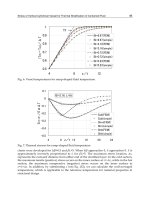
The thermal study of the transfers confirms a higher heat transfer coefficient in the input
minichannel during the phase of microgravity (Fig. 13). This decrease is due to the decrease
in size of the vapour bubbles.

Evaporation, Condensation and Heat Transfer


82
On Fig. 10 and Fig. 11, we plot the evolution of the flow in respectively terrestrial and
microgravity phase during nearly 20 seconds. We can see that there are very big differences
with the structure of the bubbles. In terrestrial gravity, we have bubbly flow profiles while
in microgravity we deal with slug and churn flow according to Fig. 7. Here, we can see the
observations made in terrestrial gravity:


Fig. 10. Flow boiling occurring in our minichannel under terrestrial gravity phase
(20 seconds, Q

w
=45 kW.m
-2
).
Then in microgravity, we observed the flow sequence which evidences a different topology
and particularly with the bubble’s size.


Fig. 11. Flow boiling occurring in our minichannel under microgravity phase (20 seconds,
Q
w
=45 kW.m
-2
).
Two Phase Flow Experimental Study Inside a Microchannel:
Influence of Gravity Level on Local Boiling Heat Transfer


83
3.3 Bubble behaviour
To understand fully the role of microgravity on flow boiling and particularly on the bubbles
patterns, we introduce the capillarity length. In fluid mechanics, capillary length is a
characteristic length scale for fluid subject to a body force from gravity and a surface force
due to surface tension. This number function of the

c
L
g
σ
=

ρ
(1)
We can see that the capillarity length depends on g
-0.5.
Or g is the only parameter that
changes during a parabola at a constant mass flow and heat flux rate. Thus when we pass
from 1g to 1.8g, L
c
decreases of 74 % whereas when we pass from 1g to µg, L
c
increases of
nearly 1400 %. This may explain the different sizes of the bubbles during microgravity.
Whatever the gravity level, as soon as the vapour occupies the entire minichannel, the heat
transfer coefficient decreases strongly to reach a level which characterizes a kind of vapour
phase heat transfer. Furthermore, as soon as the vapour completely fills the pipe, the heat
exchange strongly falls (Fig. 18). The thermal study of the transfers confirms a higher heat
transfer coefficient in the input minichannel during the phase of microgravity.
3.4 Validation
3.4.1 Kandlikar’s correlation
Very recently, (Kandlikar, 2001) proposed a correlation (see below) as a fit to a very broad
spectrum of data for flow boiling heat transfer in vertical and horizontal channels:


Fig. 12. Convective boiling heat transfer coefficient variation with quality level x (here χ
v
) for
Kandlikar’s correlation.
()
5
24

C
CC
11o le 3 K
h h C C 25Fr C Bo F
⎡
⎤
=+
⎣
⎦


0.8 0.5
v
o
1x
C
xl
−ρ
⎛⎞⎛⎞
=
⎜⎟
⎜⎟
ρ
⎝⎠
⎝⎠
(2)

Evaporation, Condensation and Heat Transfer

84
2
le
2
lh
G
Fr
g
D
=
ρ

The table below are useful to calculate the Fk number.

Fluid Fk
Water 1.00
R-11 1.30
R-12 1.50
R-13B1 1.31
R-22 2.20
Nitrogen 4.70
Neon 3.50
Fluid Fk
Water 1.00
R-11 1.30
Table 2. List of Fk values for different fluids
3.4.2 Experimental results
The results are in good agreement with the correlation (Fig. 13). Concerning the range from
0 to 5000 W.m
-2

.K
-1
, we can see that the experimental curves in terrestrial gravity have the
same curvature with the theoretical correlation. Indeed, we have the same level.


Fig. 13. Influence of vapour quality on the heat transfer coefficient in the minichannel
(Q
w
=45 kW.m
-2
).
3.4.3 Featuring experiments
We can see that we have been able to quantify the heat transfers inside our minichannels
and to validate the experimental results in normal gravity with correlation found in
literature. So for terrestrial conditions, the results are validated.
Two Phase Flow Experimental Study Inside a Microchannel:
Influence of Gravity Level on Local Boiling Heat Transfer


85
Now, we are going to present more results concerning the influence of three parameters on
the heat transfers: the gravity level, the Reynolds number and the Vapour quality. We are
presenting and analysing experimental results.
4. Heat transfer results
4.1 Inverse method
Here, we introduce quickly the estimation method to explain how we estimate our
parameter (Le Niliot, 2001). It consists in inversing experimental data measurements
(thermocouples) to obtain the surface temperature and the surface flux density in the
minichannel. The inverse problem deals with the resolution of IHCP (Beck et al, 1985) where

we want to estimate the unknown boundary conditions on the surface minichannel. The
numerical method used here is the BEM (Brebbia et al, 1984). This method has been applied
in our laboratory for several years to solve inverse problems (Le Niliot et Lefèvre, 2001).
BEM is attractive for our inverse problem resolution because it provides a direct connection
between the unknown boundary heat flux, the measurements (thermocouples here) and the
linear heat sources (heating wires here). The solution can be obtained by solving a linear
system of simultaneous equations without any iterative process.
The estimation procedure consists in inversing the temperature measurements under the
minichannel in order to estimate the local boiling heat transfer coefficient h(x), knowing the
local heat flux and the local surface temperatures (
surface
ϕ
,
surface
T ). Those functions of
space are the results of the inverse problem. The estimation of the solution is obtained as the
solution of the following optimization problem:
4.1.1 Boundary estimation
As N' is the number of domain Ω interior points given here by the thermocouples and N the
number of boundary elements on our rod, the system has got (N+N') equations. The number
of unknowns, noted M, is a function of the boundary conditions applied on the different
elements of Γ ( Fig. 14). Namely for element Γ
i
we have at least one unknown per element
for the following boundary conditions:
First kind condition for which heat flux ϕi is unknown and temperature θ
i
is imposed.
Second kind condition for which temperature θi unknown and heat flux ϕ
i

is imposed.
Third kind condition ϕi=f(θi)


Fig. 14. The problem of the unknown boundary conditions.

Evaporation, Condensation and Heat Transfer


86
The elements, for which we have one equation, where the boundary condition is missing, let
appear two unknowns. The only way to solve the fundamental heat transfer equation is to
find some extra information, provided by measurements. In our case, we have interior
measurements, given by thermocouples. They enable us with the knowledge of the
boundary conditions to solve the problem and to calculate local heat flux and local surface
temperatures along the minichannel. This estimation procedure consists in inversing the
temperature measurements under the minichannel in order to estimate the local boiling heat
transfer coefficient h(x). Those functions of space are the results of the inverse problem. The
estimation of the solution is obtained using BEM as the solution of the following
optimization problem:

()
{
}
mod meas
TT
ˆˆ
T,
surface surface
−φ =arg min (3)

In this last expression, the vectors
meas
T and
mod
T respectively represent the vector of
temperature measurements and the vector of the calculated temperatures. The unknown
factors (
surface
ϕ
,
surface
T
) are obtained by minimizing the difference between measurements
and a mathematical modeling. Taking into account the specificity of formulation BEM
., this
minimization is not obtained explicitly but done through a function utilizing a linear
combination of measurements. This formulation leads to a matrix system of simultaneous
equation :

X=BA
(4)
In this last equation,
A is a matrix of dimension ((N+N)'×M), X the vector of the M
unknowns including (
surface
ϕ
,
surface
T
) and B of dimension (N+N') is containing a linear

combination of the data measurements. If M=N+N' we obtain a square system of linear
equation but most of the time we have M<N+N' and has more equations than unknown (see
Sensitivity Study chapter) : our system presents 270 equations for 255 unknown factors
(overdetermined system). A solution can be found by minimising the distance between
vector
AX and vector B. In order to find out an estimation
ˆ
X
of the unknown exact solution
X, we have to solve the optimization problem using a cost function (5). Assuming that the
difference between
AX and B can be considered as distributed according a Gaussian law we
can find
ˆ
X
solution of in the meaning of the least squares. Using this last property leads to
the Ordinary Least Squares solution :

ˆ
⎧
⎫
⎛⎞
⎜⎟
⎨
⎬
⎝⎠
⎩⎭
2
X=arg min AX-B
(5)

()()
ˆ
X= B
TT
AA A (6)
Actually, the inverse heat condition problem is ill-posed and very sensitive to the
measurements errors. Considering the numerical aspects of the inversion, we obtain an ill-
conditioned square matrix (
A
T
A). Thus, we observe for the system numerical resolution an
instability of the solution
ˆ
X
with regards to the measurements the errors introduced into
the vector
B. As a consequence, we need to obtain a stable the solution of this system by
using regularizations tools – Hansen. We propose in the following paragraph an example of
Two Phase Flow Experimental Study Inside a Microchannel:
Influence of Gravity Level on Local Boiling Heat Transfer


87
regularization procedure which can be applied. In order to smooth the solution, we used in
our our study the Lanczos decomposition called the the SVD method.
4.1.2 Regularization using SVD
The regularization of an inverse problem consists in adding information to improve the
stability of the solution with regards to the measurements noise and/or to select a type of
solution among all those possible. The ill-conditioned character of matrix

A results in the
presence of low singular values. They are a consequence of linear dependent equations :
indication of a strong correlation between the unknown factors.
Actually, the SVD method makes possible to deal with 3D inverse problem where the mesh
is structured, i.e. the pavements of the elements do not have all the same surfaces and thus
the same sensitivity (Fig. 15). This property increased the ill-poseness of the problem.
Indeed, the solution is much more unstable when the space discretization is refined. This
singular behavior is due to the fact that the conditioning number of the linear system (see
the L-curve paragraph) is a function of the power of the meshing step.

0
Fig. 15. 3D Meshing- of the minichannel only the faces are meshed.
In our problem, SVD method consists in removing the too small singular values which affect
the stability of the system in order to find one solution among several, which best
corresponds. It can seem contradictory to improve the system by removing equations and
thus information : the suppression of the equations involves a reduction in the rank of our
system and consequently an increase in the space of the plausible solutions. However, the
action of removing these equations improves the stability because it deliberately removes
the equations which disturb the solution. Matrix
A can be built into a product of squares
matrices (
U and V are orthogonal matrices and W is the diagonal matrix of the singular
values
w
j
) as shown :

Evaporation, Condensation and Heat Transfer

88
T
AUWV=

T
j
1
XUDia
g
VB
w
⎛⎞
⎛⎞
⎜⎟
⎜⎟
=
⎜⎟
⎜⎟
⎝⎠
⎝⎠
(7)
A is ill-conditioned when some singular values w
j
→ 0 (1/w
j
→ ∞ ).As a result, the errors are
increased. By using SVD, W
-1
is truncated from the too high (1/w
j

).

1
n
w
0
W
0
w
0
⎡
⎤
⎢
⎥
⎢
⎥
⎢
⎥
=
⎢
⎥
⎢
⎥
⎢
⎥
⎣
⎦
""
#% #
#%#

#%
"""
(8)
The truncated matrix can be built up as in:

1
t
p
w
0
W
0
w
0
0
⎡
⎤
⎢
⎥
⎢
⎥
⎢
⎥
=
⎢
⎥
⎢
⎥
⎢
⎥

⎣
⎦
""
#% #
#%#
""
(9)
The estimate solution vector
ˆ
X
is function of the new truncated matrix
1
t
W
−
:

(
)
T1
t
ˆ
XUWVB
−
=
(10)
We observe like in the regularization method by modifications of the functions to be
minimised (for example Tikhonov) a smoothing of the solution. However, it is necessary to
explain how is carried out the choice of the singular values ignored. There is a “criteria”
making it possible to quantify the balance between a stable solution and low residuals : the

condition number. It is defined by the ratio of the highest to the weakest of the singular
values of matrix A.
All the singular values lower than a limit value are eliminated. The numerical procedure can
be found in the LINPACK or in Numerical recipes (Press et al, 1990). This technique requires
the use of a threshold which allows the choice of values to be cancelled. The level of
truncation is determined by the technique known as the L-curve (Hansen, 1998).
4.1.3 The L-curve
The obtained solution
ˆ
X
depends on a value selected by the user. To avoid entering
extremes and losing information, a tool called L-curve is introduced to estimate the correct
condition number. The goal is to trace on a logarithmic scale the norm of the solution on the
norm of the residuals
AX-B
ˆ
(Fig. 16).
The optimal value is in the hollow of the L where the best compromise between stable
results and low residuals (on the distinct corner separating the vertical and the horizontal
part of the curve). It is around this corner that we find the best compromise.
Two Phase Flow Experimental Study Inside a Microchannel:
Influence of Gravity Level on Local Boiling Heat Transfer


89
Thus, this value makes it possible to define the truncation level and the number of
conditioning associated. In our problem, this value is around 10
7
, which is very high and
shows how ill-posed our system is.

Fig. 16. L-Curve approach applied to the B.E.M
4.2 Local estimation
Knowing the estimated surface temperatures (
surface
ˆ
T
) and the surface heat flux (
surface
ˆ
ϕ ),
we can calculate the local boiling coefficient
ˆ
h
in the minichannel knowing the saturation
temperature of the liquid (
sat
T ):

()
()
surface
surface sat
ˆ
x
ˆ
h
ˆ
TxT
φ

=
−
(11)
On Fig. 17
, we show the evolution of the local wall temperature and the heat flux function of
the minichannel length:

Fig. 17. Influence of gravity on the surface temperature and the heat flux along the
minichannel (Q
w
=33 kW.m
-2
).

Evaporation, Condensation and Heat Transfer


90
We observe that the temperature profile increases and that in microgravity, the values are
higher. The temperature rises, which is agreement with the temperatures distribution that
we used in the inversion procedure. Then we can easily plot the local heat transfer
coefficient function of the minichannel length:


Fig. 18. Influence of gravity on the heat transfer coefficient along the minichannel (Q
w
=45
kW.m
-2
).

First result shows that during the microgravity period, in inlet of the minichannel (x=20
mm), the heat transfer coefficient is higher with a value around 15000 W.m
-2.
K
-1
. This value
has to be compared to the 1.8g and the 1g where it is equal to 7500 W.m
-2.
K
-1
. Second result
indicates that it decreases along the x length in the flow direction. Whatever the gravity
level, as soon as the vapour occupies the entire minichannel, the heat transfer coefficient
decreases strongly to reach a level which characterizes a kind of vapour phase heat transfer.
Furthermore, as soon as the vapour completely fills the pipe, the heat exchange strongly
falls because there is no more liquid boiling (Fig. 18) but only heat transfer through the
vapour (heat insulator).
4.3 Reynolds number
Fig. 19 presents the evolution of the heat transfer coefficient as a function of the Reynolds
number. In our configuration, we are in a laminar flow and the curve behaviour is
observed for all studied gravity level. Here, we plot the results for a constant heat flux.
We can observe two significant results: with the increasing Reynolds number, the heat
transfer coefficient increases for each gravity level. Secondly, the average heat transfer
coefficient is higher in microgravity. Knowing this, we can propose a global behaviour of
the fluid flow in the minichannel. Nucleate boiling is the dominant vaporization
mechanism near the onset of boiling. As more vapours are generated in the flow and the
void fraction increases, evaporation from the liquid-vapour interface becomes
increasingly important.
Two Phase Flow Experimental Study Inside a Microchannel:
Influence of Gravity Level on Local Boiling Heat Transfer

91

Fig. 19. Influence of Reynolds number on the average heat transfer coefficient in the
minichannel (Q
w
=45 kW.m
-2
).
4.4 Local quality
We plot the local vapour quality as a function of the x-axis of the minichannel using the
following equation:

w
v
vl v
Qx
(x)
SL u
χ=
ρ
(12)
First results (Fig. 20
) show that the local quality increases along the main axis from the inlet
to the outlet of the channel. This is in good agreement with the temperature profile we have
on the boundary minichannel since at the outlet the temperature is higher (Fig. 17).


Fig. 20. Influence of local vapor quality as a function of the main flow axis (Q

w
=45 kW.m
-2
).

Evaporation, Condensation and Heat Transfer


92
A second result shows a non linear evolution because in our case the heat flux density is not
constant. Indeed, the Q
W
calculated on the wall minichannel varies around 2 %. This result
is explicit at the inlet minichannel where we observe a short decrease since the error
estimation is higher around these points. Besides, at the outlet minichannel, the local vapour
quality (x=60 mm) tends to reach a value corresponding to the global outlet vapour quality.

v
out
w
v
Total
w
Q
Q
⎛⎞
χ=
⎜⎟
⎜⎟
⎝⎠

(13)
When we are at the edges of our channel, the local value is close to the outlet vapour quality:

out
vv
xL
lim (x)
→
χ
=
χ
(14)
Where x is the abscissa of the minichannel and L is the final length. This comparison is used
to validate our results. Here, we have plot four tends of the local vapour quality as a
function of the minichannel axis. We observe on Fig. 13, that the heat transfer coefficient
profile for the terrestrial gravity decreases when the vapour quality increases. This is in
good agreement with our experimental data under terrestrial gravity conditions. Indeed, as
quality increases, the Kandlikar correlation predicts a steadily decreasing heat transfer
coefficient. The nucleate boiling contribution diminishes while the forced-convective effect
decreases and there is a steady drop in heat transfer coefficient with quality. However, the
experimental results can only be compared during terrestrial gravity because when we are
in microgravity and hypergravity, the correlations is no longer valid. Actually, we can't find
a model that predicts the behaviour of the boiling heat transfer coefficient when the gravity
level changes. Plus, with the increasing Re, the outlet vapour fraction is decreasing meaning
that the average vapour fraction is lower and dry out has less influence on heat transfer.
5. Conclusion and perspectives
A study of two-phase flow regimes in a vertical rectangular minichannel is performed.
Actually, flow boiling heat transfer in microgravity has received relatively little attention.
Thus, the few experiments and the short duration of microgravity conditions do not allow a
full understanding of the mechanisms controlling flow boiling heat transfers. But it is a

starting point. In this study, we gathered all the results highlighted the influence of gravity
on convective boiling in minichannels. Local values of wall surface temperature; heat flux
and heat transfers were done and helped us to construct boiling curves. We perform
analysis of the selected parameters which influence the mechanisms. Indeed, the analysis of
temperature as a function of g confirms that gravity has an influence on flow and heat
transfer. The microgravity generates vapour pocket structures which fill the width of the
minichannel and the heat transfer coefficient is locally higher. Consequently, we can assume
that microgravity influences the appearance of the vapour bubbles whose size varies
depending parameter g. In the case of hypergravity and normal gravity, a classical bubbly
flow structure is observed. Concerning the inverse method, we were able to solve a 3D
IHCP. For the inverse methods, the sensors induce too many disturbances and accentuate
the ill-posed character. These uncertainties lead to clear variations in the solution and
particularly in the surface heat flux. One solution would be to add IR (infra-red)
Two Phase Flow Experimental Study Inside a Microchannel:
Influence of Gravity Level on Local Boiling Heat Transfer


93
measurements while painting the lower face of the cement in black and placing a camera
directly below and another would be to destroy the minichannels to estimate the locations of
the thermocouples. In addition, all the experimental data are not totally transient. Indeed,
we have some gravity phase changes which are steady so that using a normal steady
approach to study convective boiling was successfully done. Thus, to use all our
experimental data and to confirm our results, prediction of the convective boiling heat
transfer coefficient requires a transient approach. That’s why we need to take into account
these dynamic instabilities for further results. In outgoing experiments, to deal with more
experimental data from the Parabolic Flight campaign, we will perform this transient
formulation.
6. Acknowledgment
We would especially like to thank the CNES (793/2002/CNES/8665) and ESA (MAP

Boiling) for their financial support. We thank them for giving us access to the
experimentation in microgravity on board the A300 Zero-G. We would also like to express
our gratitude to Novespace® and more especially to Mr. Mora and Mr. Gai for their
technical assistance during the campaigns PF52/CNES and PF53/ESA
7. References
Carey V. P. (1992). Liquid-Vapour Phase Change Phenomena, Hemisphere Publishing
Corporation, New York
Kandlikar S. G.(2001). Fundamental issues related to flow boiling in minichannels and
microchannels, Experiental Heat Transfer, Fluid Mechanics and Thermodynamics,
Vol.1, Edizioni ETS, PISA, 2001.
Tadrist L. (October 2007). Flow Boiling in Microgravity Condition: Investigation Using
Inverse Techniques.
J. of Microgravity Science and Technology, October 26-28.
Yan Y. and Kenning D. B. R.(1998) Pressure fluctuations during boiling in a narrow channel.
HTFS Research Symposium.
Kennedy J. E., Roach G. M., Dowling M. F., Abdel-Khalik S. I., Ghiaasiaan S. M., Jeter S. M.,
and Quershi Z. H.(February 2000). The onset of flow instability in uniformly heated
horizontal microchannels.
Journal of Heat Transfer, 122:118–125.
Qu W., Mudawar I. (2003). Flow boiling heat transfer in two-phase micro-channel heat
sinks: Experimental investigation and assessment of correlations methods.
International Journal of Heat and Mass Transfer, 46.
Brutin D. and Tadrist L. (October 2006). Destabilization mechanisms and scaling laws of
convective boiling in a minichannel. AIAA
Journal of Thermophysics and Heat
Transfers, 20.
Hestroni G. et al.(2005). Fluid flow in microchannels.
International Journal of Heat and Mass
Transfer
, pages 1982-1998.

Tran T.N., Wambsganss M.W. and D.M. (1996). Small circular and rectangular channel
boiling with two refrigerants,
International Journal of Multiphase Flow, pages 485-498.
Thome J.R. (2004). Boiling in microchannels: a review of experiment and theory.
International
Journal of Heat and Fluid Flow, pages 128-139.
Kew P.A. and Cornwell K. (1997). Correlations for the prediction of boiling heat transfer in
small-diameter channels.
Applied Thermal Engineering, pages 705-715.