Developments in Heat Transfer Part 5 docx

Variable Property Effects in Momentum and Heat Transfer

149
This is also true with respect to the field variables of these cases. For example, Fig. 7 shows
that there is an appreciable difference when the temperature field is calculated by DNS
compared to the RANS results.
However, as shown in Fig. 8, the iso-temperature lines for variable properties, calculated by
DNS are well represented by iso-lines from the AD-HOC method, i.e. those lines from
constant property DNS results corrected by A-values from RANS solutions for variable
properties.




Fig. 8. Variable property results of the temperature field in a differentially heated cavity, see
Fig. 4,
8
Ra 2 10=×
Distribution of the first order A-values
A
γ
, A
μ
,
k
A
and
p
c
A

, computed by RANS, are
shown in Fig. 9. The variable properties behave differently in the core region, where a quasi-
laminar flow prevails and in the large vortex region near the bottom and top walls. Also,
signs within one region are different. For example
A
γ
and A
μ
are negative in the core
DNS, constant properties
DNS, variable properties
DNS, AD-HOC method

Developments in Heat Transfer

150
region, whereas
k
A and
p
c
A are positive in the same region. Altogether there is a non-
negligible effect of variable properties on the temperature distribution.





Fig. 9. A-values of temperature computed by RANS in a differentially heated cavity, see
Fig. 4,

8
Ra 2 10=× (a) A
γ
; (b) A
μ
; (c)
k
A ; (d)
p
c
A
(a)
(b)
(c)
(d)
A
γ
A
μ

k
A
p
c
A

Variable Property Effects in Momentum and Heat Transfer

151
5. Conclusions

Various methods to account for variable property effects in complex geometries and highly
sophisticated numerical methods have been proposed. Due to the Taylor series expansions
of all properties, which are the starting point for all methods, the influence of variable
properties can be accounted for in a general manner, i.e. for all (small) heating rates and for
all Newtonian fluids. For a special problem with A-values determined once, the effect of
variable properties can be found in the final result by fixing
ε
(the heat transfer rate) and all
K-values (from the fluid of interest).
This way of treating variable property effects is much closer to the physics than empirical
methods like the property ratio and the reference temperature methods are.
6. Nomenclature
2
,,,
aaaaba
A
AAA

A-values,
{
}
,,,,,,
p
ab kc a b
ργ μ
∈
≠
p
c specific heat capacity
f

friction factor
g
G
gravity vector
a
j
h h-values,
j
a
j
K
ε

j empirical parameter
2
,,
aa an
KK K
K-values, , , , ,
p
akc
ρ
γμ
=

k heat conductivity
*
L characteristic length
,
aa

mn empirical exponents
Nu Nußelt number
p
pressure
Pr Prandtl number
a
P nondimensional properties about variable fluid property
q

heat flux
Re
Reynolds number
T temperature
u
G
velocity vector
V variables
Greek symbols
,,,
α
βσδ
variables composed of fluid properties
γ
expansion coefficient
*
TΔ temperature difference
ε
nondimensional temperature difference
μ
dynamic viscosity

ρ
density
subscripts
c
p
constant properties
R reference state
* dimensional

Developments in Heat Transfer

152
7. Acknowledgement
This study was supported by the DFG (Deutsche Forschungsgemeinschaft).
8. References
Bünger F. & Herwig H. (2009). An extended similarity theory applied to heated flows in
complex geometries.
ZAMP, Vol. 60, (2009), pp. 1095-1111.
Carey V. P. & Mollendorf J. C. (1980). Variable viscosity effects in several natural convection
flows.
Int. J. Heat Mass Transfer, Vol. 23, (1980), pp. 95-109
Debrestian D. J. & Anderson J. D. (1994). Reference Temperature Method and Reynolds
Analogy for Chemically Reacting Non-equilibrium Flowfields.
J. of Thermophysics
and Heat Transfer,
Vol. 8, (1994), pp. 190-192
Herwig H. & Wickern G. (1986). The Effect of Variable Properties on Laminar Boundary
Layer Flows.
Wärme- und Stoffübertragung, Vol. 20, (1986), pp. 47-57
Herwig H. & Bauhaus F. J. (1986). A Regular Perturbation Theory for Variable Properties

Applied to Compressible Boundary Layers.
Proceedings of 8
th
International Heat
Transfer Conference
, San Fransisco, Vol. 3, 1095-1101, 1986
Herwig H., Voigt M. & Bauhaus F. J. (1989). The Effect of Variable Properties on Momentum
and Heat Transfer in a Tube with constant Wall Temperature.
Int. J. Heat Mass
Transfer
, Vol. 32, (1989), pp. 1907-1915
Herwig H. & Schäfer P. (1992). Influence of variable properties on the stability of two-
dimensional boundary layers.
J. Fluid Mechanics, Vol. 243, (1992), pp. 1-14.
Jayari S.; Dinesh K. K., & Pillai K. L. (1999). Thermophoresis in natural convection with
variable properties.
Heat and Mass Transfer, Vol. 35, (1999), pp. 469-475
Jin Y. & Herwig H. (2010). Application of the Similarity Theory Including Variable Property
Effects to a Complex Benchmark Problem,
ZAMP, Vol. 61, (2010), pp. 509-528
Jin Y. & Herwig H. (2010). Efficient method to account for variable property effects in
numerical momentum and heat transfer solutions,
Int. J. Heat Mass Transfer, (2011),
in press
Li Z.; Huai X.; Tao Y. & Chen H. (2007). Effects of thermal property variations on the liquid
flow and heat transfer in micro-channel heat sinks.
Applied Thermal Engineering, Vol.
27 (2007), pp. 2803–2814
Mahmood G. I.; Ligrani P. M. & Chen K. (2003). Variable property and Temperature Ratio
Effects on Nusselt Numbers in a Rectangular Channel with 45 Deg Angle Rib

Turbulators.
J. Heat Transfer, Vol. 125 (2003), pp. 769-778
Trias F. X.; Soria M.; Oliva A. & Pérez-Segarra C. D. (2007). Direct numerical simulations of
two- and three-dimensional turbulent natural convection flows in a differentially
heated cavity of aspect ratio 4,
J. Fluid Mech., Vol. 586, (2007), pp. 259–293
Trias F. X.; Gorobets A.; Soria M. & Oliva A. (2010a). Direct numerical simulation of a
differentially heated cavity of aspect ratio 4 with Rayleigh numbers up to 1011 –
Part I: Numerical methods and time-averaged flow,
International Journal of Heat and
Mass Transfer
, Vol. 53, (2010), pp. 665–673
Trias F. X.; Gorobets A.; Soria M. & Oliva A. (2010b). Direct numerical simulation of a
differentially heated cavity of aspect ratio 4 with Rayleigh numbers up to 1011 –
Part II: Numerical methods and time-averaged flow,
International Journal of Heat and
Mass Transfer
, Vol. 53, (2010), pp. 674–683
9
Bioheat Transfer
Alireza Zolfaghari
1
and Mehdi Maerefat
2

1
Department of Mechanical Engineering, Birjand University, Birjand,
2
Department of Mechanical Engineering, Tarbiat Modares University, Tehran,
Iran

1. Introduction
Heat transfer in living tissues is a complicated process because it involves a combination of
thermal conduction in tissues, convection and perfusion of blood, and metabolic heat
production. Over the years, several mathematical models have been developed to describe
heat transfer within living biological tissues. These models have been widely used in the
analysis of hyperthermia in cancer treatment, laser surgery, cryosurgery, cryopreservation,
thermal comfort, and many other applications. The most widely used bioheat model was
introduced by Pennes in 1948. Pennes proposed a new simplified bioheat model to describe
the effect of blood perfusion and metabolic heat generation on heat transfer within a living
tissue. Since the landmark paper by Pennes (1948), his model has been widely used by many
researchers for the analysis of bioheat transfer phenomena. And, also a large number of
bioheat transfer models have been proposed to overcome the shortcomings of Pennes’
equation. These models include the continuum models which consider the thermal impact
of all blood vessels as a global parameter and the vascular models which consider the
thermal impact of each vessel individually.
Although, several bioheat models have been developed in the recent years, the
thermoregulatory control mechanisms of the human body such as shivering, regulatory
sweating, vasodilation, and vasoconstriction have not been considered in these models. On
the other hand, these mechanisms may significantly influence the thermal conditions of the
human body. This causes a serious limitation in using the bioheat models for evaluating the
human body thermal response. In order to remove this limitation, Zolfaghari and Maerefat
(2010) developed a new Simplified Thermoregulatory Bioheat (STB) model based on the
combination of the well-known Pennes’ equation and Gagge’s thermal comfort model.
The present chapter aims at giving a concise introduction to bioheat transfer and the
mathematical models for evaluating the heat transfer within biological tissues. This chapter
is divided into six sections. The first section presents an introduction to the concept and
history of bioheat transfer. The structure of living tissues with blood perfusion is described
in section 2. Next, third section focuses on the mathematical modelling of heat transfer in
living tissues. In the mentioned section, a brief description of some of the most important

bioheat models (i.e. Pennes (1948) model, Wulff (1974) model, Klinger (1974) model, Chen
and Holmes (1980) model and so on) is presented. Afterwards, section 4 explains the
complexity of evaluating heat transfer within the tissues that thermally controlled by
thermoregulatory mechanisms such as shivering, regulatory sweating, vasodilation, and

Developments in Heat Transfer

154
vasoconstriction. Then, the Simplified Thermoregulatory Bioheat (STB) model is introduced
for evaluating heat transfer within the segments of the human body. Finally, section 5
outlines the main conclusions and recommendations of the research. Moreover, the selected
references are listed in the last section.
2. Structure of blood perfused tissues
Before we discuss the bioheat models, let us have a brief look at the structure of blood
perfused tissues. The biological tissues include the layers of skin, fat, muscle and bone.
Moreover, the skin is composed of two stratified layers: epidermis and dermis. Fig. 1 shows
a schematic geometry of the tissue structure. Furthermore, the thermophysical properties of
the human body tissue are provided in Table 1 (Lv & Liu, 2007; Sharma, 2010).


Fig. 1. Schematic geometry of the tissue structure (figure not to scale)

Thickness Density
Specific
heat
Blood perfusion
rate
Thermal
conductivity
l (m)

ρ
(kg/m
3
)
C (J/kg K) W
bl
(m
3
/s m
3
) k (W/m K)
Epidermis 80×10
-6
1200 3589 0 0.24
Dermis 0.002 1200 3300 0.00125 0.45
Fat
≈ 0.010
937 3258 0.00125 0.21
Muscle
≈ 0.020
1000 4000 0.00125 0.5
Bone
≈ 0.008
1920 1440 - 0.44
Blood - 937 3889 - 0.64
Table 1. Geometrical information and thermal properties of the human body tissue (Lv & Liu,
2007; Sharma, 2010)
Blood circulation is a key mechanism for regulating the body temperature. The circulatory
system of the human body comprises of two sets of blood vessels (arteries and veins) which
carry blood from the heart and back. Blood leaves the heart through the aorta, which is the

largest artery (diameter ≈ 5000 μm). Vessels supplying blood to muscles are known as main
supply arteries and veins (SAV, 300-1000 μm diameter). They branch into primary arteries,
(P, 100-300 μm diameter) which feed the secondary arteries (s, 50-100 μm diameter). These

Bioheat Transfer

155
vessels deliver blood to the arterioles (20-40 μm diameter) which supply blood to the
smallest vessels known as capillaries (c, 5-15μm diameter). Blood is returned to the heart
through a system of vessels known as veins. Fig. 2 shows a schematic diagram of a typical
vascular structure (Jiji, 2009).


Fig. 2. Schematic diagram of the vascular system (Jiji, 2009)


Fig. 3. Schematic of temperature equilibration between the blood and the tissue (Datta, 2002)

Developments in Heat Transfer

156
Blood leaves the heart at the arterial temperature T
art
. It remains essentially at this
temperature until it reaches the main arteries where equilibration with surrounding tissue
begins to take place. Equilibration becomes complete prior to reaching the arterioles and
capillaries. Beyond this point, blood temperature follows the solid tissue temperature (T
ti
)
through its spatial and time variations until blood reaches the terminal veins. At this point

the blood temperature ceases to equilibrate with the tissue, and remains virtually constant,
except as it mixes with other blood of different temperatures at venous confluences. Finally,
the cooler blood from peripheral regions and warmer blood from internal organs mix within
the vena cava and the right atrium and ventricle. Following thermal exchange in the
pulmonary circulation and remixing in the left heart, the blood attains the same temperature
it had at the start of the circuit (Datta, 2002). Fig. 3 shows a schematic of temperature
equilibration between the blood and the solid tissue.
3. Mathematical models of bioheat transfer
3.1 Pennes model
Over the years, the effects of blood flow on heat transfer in living tissue have been studied
by many researchers and a large number of bioheat transfer models have been developed on
the basis of two main approaches: the continuum approach and the discrete vessel
(vascular) approach. In the continuum approach, the thermal impact of all blood vessels
models with a single global parameter; and the vascular approach models the impact of
each vessel individually (Raaymakers et al., 2009). The most widely used continuum model
of perfused tissue was introduced in 1948 by Harry Pennes. The Pennes (1948) model was
initially developed for predicting heat transfer in the human forearm. Due to the simplicity
of the Pennes bioheat model, it was implemented in various biological research works such
as for therapeutic hyperthermia for the treatment of cancer (Minkowycz et al., 2009).
Pennes bioheat model is based on four simplifying assumptions (Jiji, 2009):
1. All pre-arteriole and post-venule heat transfer between blood and tissue is neglected.
2. The flow of blood in the small capillaries is assumed to be isotropic. This neglects the
effect of blood flow directionality.
3. Larger blood vessels in the vicinity of capillary beds play no role in the energy
exchange between tissue and capillary blood. Thus the Pennes model does not consider
the local vascular geometry.
4. Blood is assumed to reach the arterioles supplying the capillary beds at the body core
temperature. It instantaneously exchanges energy and equilibrates with the local tissue
temperature.
Based on these assumptions, Pennes (1948) modeled blood effect as an isotropic heat source

or sink which is proportional to blood flow rate and the difference between the body core
temperature and local tissue temperature. Therefore, Pennes (1948) proposed a model to
describe the effects of metabolism and blood perfusion on the energy balance within tissue.
These two effects were incorporated into the standard thermal diffusion equation, which is
written in its simplified form as:

ti
ti ti ti ti bl bl bl art ti m
.()
T
CkTCWTTq
t
ρρ
∂
=∇ ∇ + − +
∂
(1)
where ρ
ti
, C
ti
, T
ti
and k
ti
are, respectively, the density, specific heat, temperature and thermal
conductivity of tissue. Also, T
art
is the temperature of arterial blood, q
m

is the metabolic heat

Bioheat Transfer

157
generation and ρ
bl
, C
bl
and W
bl
are, respectively, the density, specific heat and perfusion rate
of blood. It should be noted that metabolic heat generation is assumed to be homogeneously
distributed throughout the tissue. Also, it is assumed that the blood perfusion effect is
homogeneous and isotropic and that thermal equilibration occurs in the microcirculatory
capillary bed. In this scenario, blood enters capillaries at the temperature of arterial blood,
T
art
, where heat exchange occurs to bring the temperature to that of the surrounding tissue,
T
ti
. There is assumed to be no energy transfer either before or after the blood passes through
the capillaries, so that the temperature at which it enters the venous circulation is that of the
local tissue (Kreith, 2000).
Pennes (1948) performed a series of experimental studies to validate his model. Validations
have shown that the results of Pennes bioheat model are in a reasonable agreement with the
experimental data. Although Pennes bioheat model is often adequate for roughly describing
the effect of blood flow on the tissue temperature, there exist some serious shortcomings in
his model due to its inherent simplicity. The shortcomings of Pennes bioheat model come
from the basic assumptions that are introduced in this model. These shortcomings can be

listed as follows (Jiji, 2009):
1. Thermal equilibration does not occur in the capillaries, as Pennes assumed. Instead it
takes place in pre-arteriole and post-venule vessels having diameters ranging from 70-
500 μm.
2. Directionality of blood perfusion is an important factor in the interchange of energy
between vessels and tissue. The Pennes equation does not account for this effect.
3. Pennes equation does not consider the local vascular geometry. Thus significant
features of the circulatory system are not accounted for. This includes energy exchange
with large vessels, countercurrent heat transfer between artery-vein pairs and vessel
branching and diminution.
4. The arterial temperature varies continuously from the deep body temperature of the
aorta to the secondary arteries supplying the arterioles, and similarly for the venous
return. Thus, contrary to Pennes’ assumption, pre-arteriole blood temperature is not
equal to body core temperature and vein return temperature is not equal to the local
tissue temperature. Both approximations overestimate the effect of blood perfusion on
local tissue temperature.
To overcome these shortcomings, a considerable number of modifications have been
proposed by various researchers. Wulff (1974) and Klinger (1974) considered the local blood
mass flux to account the blood flow direction, while Chen and Holmes (1980) examined the
effect of thermal equilibration length on the blood temperature and added the dispersion
and microcirculatory perfusion terms to the Klinger equation (Vafai, 2011). In the following
sections, a brief review of the modified bioheat models will be given.
3.2 Wulff continuum model
Due to the simplicity of the Pennes model, many authors have looked into the validity of the
assumptions used to develop the Pennes bioheat equation. Wulff (1974) was one of the first
researchers that directly criticized the fundamental assumptions of the Pennes bioheat
equation and provided an alternate analysis (Cho, 1992). Wulff (1974) assumed that the heat
transfer between flowing blood and tissue should be modeled to be proportional to the
temperature difference between these two media rather than between the two bloodstream
temperatures (i.e., the temperature of the blood entering and leaving the tissue). Thus, the

energy flux at any point in the tissue should be expressed by (Minkowycz et al., 2009)

Developments in Heat Transfer

158

ti ti bl bl h
qkT hv
ρ
=
−∇ + (2)
where v
h
is the local mean blood velocity. Moreover, h
bl
is the specific enthalpy of the blood
and it is given by

bl
o
**
bl bl bl bl f
bl
()d (1 )
T
T
P
hCTT H
φ
ρ

=
++Δ −
∫
(3)
where P is the system pressure, ΔH
f
is the enthalpy of formation of the metabolic reaction,
and
φ
is the extent of reaction. Also, T
o
and T
bl
are the reference and blood temperatures,
respectively. Thus, the energy balance equation can be written as

ti
ti ti
.
T
Cq
t
ρ
∂
=
−∇
∂
(4)
Therefore,

bl
o
**
ti
ti ti ti ti bl h bl bl bl f
bl
.()d(1)
T
T
T
P
CkTvCTTH
t
ρρ φ
ρ
⎡
⎤
⎛⎞
∂
=−∇ − ∇ + + +Δ −
⎢
⎥
⎜⎟
∂
⎢
⎥
⎝⎠
⎣
⎦
∫

(5)
Neglecting the mechanical work term (P/
ρ
bl
), setting the divergence of
bl h
v
ρ
to zero, and
assuming constant physical properties, Eq. (5) can be simplified as follows (Minkowycz et
al., 2009):

2
ti
ti ti ti ti bl bl h bl bl h f
T
CkTCvTvH
t
ρ
ρρφ
∂
=
∇− ∇+ Δ∇
∂
(6)
Since blood is effectively microcirculating within the tissue, it will likely be in thermal
equilibrium with the surrounding tissue. As such, Wulff (1974) assumed that
T
bl
is

equivalent to the tissue temperature
T
ti
. In this condition, the metabolic reaction term
(
bl h f
vH
ρ
φ
Δ∇) is equivalent to q
m
. Therefore, the final form of the bioheat equation that was
derived by Wulff (1974) is

2
ti ti ti ti bl bl h ti m
.
T
CkTCvTq
t
ρρ
∂
=∇ − ∇+
∂
(7)
It should be noted that the main challenge in solving this bioheat equation is in the
evaluation of the local blood mass flux
bl h
v
ρ

(Minkowycz et al., 2009).
3.3 Klinger continuum model
In 1974, Klinger presented an analytical bioheat model that was conceptually similar to
Wulff bioheat model. Klinger (1974) argued that in utilizing the Pennes model, the effects of
nonunidirectional blood flow were being neglected and thus significant errors were being
introduced into the computed results. In order to correct this lack of directionality in the
formulation, Klinger (1974) proposed that the convection field inside the tissue should be
modeled based upon the
in vivo vascular anatomy (Cho, 1992). Taking into account the
spatial and temporal variations of the velocity and heat source, and assuming constant
physical properties of tissue and incompressible blood flow, the Klinger bioheat equation
was expressed as:

Bioheat Transfer

159

2
ti ti ti ti bl bl ti m
v.
T
CkTCT
q
t
ρρ
∂
=∇ − ∇+
∂
(8)
This equation is similar to that derived by Wulff (1974), except it is written for the more

general case of a spatially and temporally nonuniform velocity field (v) and heat source (q
m
).
3.4 Chen-Holmes (CH) continuum model
Among the continuum bioheat models, the Chen-Holmes model (Chen & Holmes, 1980) is
the most developed (Kreith, 2000). Chen and Holmes (1980) showed that the major heat
transfer processes occur in the 50 to 500μm diameter vessels. Consequently, they proposed
that larger vessels be modeled separately from smaller vessels and tissue. Therefore, in the
Chen-Holmes bioheat model, the total tissue control volume is subdivided to the solid-
tissue subvolume (V
s
) and blood subvolume (V
b
) as shown in Fig. 4. By using this concept,
Chen and Holmes (1980) proposed a new modified relationship for calculating the blood
perfusion term (q
bl
) in their bioheat model:

**
bl bl bl bl art ti bl bl ti p ti
()v qCWTTCTkT
ρρ
=−−∇+∇∇
(9)


Fig. 4. Schematic representation of tissue control volume as used in Chen-Holmes model
(Kreith, 2000)
In Eq. (9), the first term on the right hand side appears similar to Pennes’ perfusion term

except the perfusion rate (
*
bl
W ) and the arterial temperature (
*
art
T ) are specific to the volume
being considered. It should be noted that
*
art
T is essentially the temperature of blood
upstream of the arterioles and it is not equal to the body core temperature. The second term
in Eq. (9) accounts for energy convected due to equilibrated blood. Directionality of blood
flow is described by the vector
v, which is the volumetric flow rate per unit area. The third
term in Eq. (9) describes conduction mechanisms associated with small temperature
fluctuations in equilibrated blood. The symbol
k
p
denotes “perfusion conductivity”. It is a
function of blood flow velocity, vessel inclination angle relative to local temperature
gradient, vessel radius and number density.
Using a simplified volume-averaging technique, the Chen-Holmes bioheat equation can be
written as follows:

{}
**
ti
ti,eff ti,eff ti,eff ti bl bl bl art ti bl bl ti p ti m
.()v

T
CkTCWTTCTkTq
t
ρρρ
∂
=∇ ∇− − − ∇+∇∇ +
∂
(10)

Developments in Heat Transfer

160
where

ti,eff bl ti bl bl
(1 )
ρ
ερ ερ
=
−+ (11)

ti,eff bl ti bl bl
(1 )CCC
ε
ε
=
−+ (12)

ti,eff bl ti bl bl
(1 )kkk

ε
ε
=
−+ (13)
where
bl
ε
is the porosity of the tissue where blood flows and
*
ti
T is the local mean tissue
temperature expressed as (Minkowycz et al., 2009)

*
bl ti ti ti bl bl bl bl
ti
ti,eff ti,eff
(1 ) CT C k
T
C
ερ ερ
ρ
−+
= (14)
Since
bl
ε
<<1, it follows that k
ti,eff
is independent of blood flow and equal to the conductivity

of the solid tissue (k
ti
).
Although the Chen-Holmes model represents a significant improvement over Pennes’
equation, it is not easy to implement since it requires detailed knowledge of the vascular
network and blood perfusion. Furthermore, the model does not explicitly address the effect
of closely spaced countercurrent artery-vein pairs (Kreith, 2000).
3.5 Weinbaum, Jiji and Lemons (WJL) bioheat model
The modeling of countercurrent vascular system, which was not explicitly addressed by the
Chen-Holmes model, developed separately from that of the continuum models. In 1984,
Weinbaum, Jiji and Lemons presented a new vascular bioheat model by considering the
countercurrent blood flow. This model was obtained based on a hypothesis that small
arteries and veins are parallel and the flow direction is countercurrent, resulting in
counterbalanced heating and cooling effects (Fig. 5). It should be noted that this assumption
is mainly applicable within the intermediate tissue of the skin (Minkowycz et al., 2009). In
an anatomic study performed on rabbit limbs, Weinbaum et al. (1984) identified three
vascular layers (deep, intermediate, and cutaneous) in the outer 1cm tissue layer. For the
countercurrent structure of the deep tissue layer, they proposed a system of three coupled
equations:

2
art
bl bl art
d
v.
d
T
Cr q
s
ρπ

=− (15)

2
v
bl bl v
d
v.
d
T
Cr q
s
ρπ
=
− (16)

2
ti art v
ti ti ti ti bl bl art v bl bl m
d( )
.()v.
d
TTT
CkTngCTTCnr q
ts
ρρρπ
∂−
⎧⎫
=∇ ∇ + − − +
⎨⎬
∂

⎩⎭
(17)
where q
art
is the heat loss from the artery by conduction through its wall, q
v
is the heat gain
by conduction per unit length through the vein wall into the vein, T
art
and T
v
are the bulk
mean temperatures inside the blood vessel, r is the vessel radius,
v is the mean velocity in
either the artery or vein, n
is the number of arteries or veins, and g is the perfusion bleed-off

Bioheat Transfer

161
velocity per unit vessel surface area (s). The first two equations describe the heat transfer of
the thermally significant artery and vein, respectively. The third equation refers to the tissue
surrounding the artery–vein pair. In Eq. (17), the middle two right-hand-side terms
represent the capillary bleed-off energy exchange, and the net heat exchange between the
tissue and artery–vein pair, respectively. The capillary bleed-off term is similar to Pennes’
perfusion term except the bleed-off mass flow (
g) is used. Their analysis showed that the
major heat transfer is due to the imperfect countercurrent heat exchange between artery–
vein pairs. They quantified the effect of perfusion bleed-off associated with this vascular
structure, and showed that Pennes’ perfusion formulation is negligible due to the

temperature differential (Kreith, 2000).


Fig. 5. Schematic of artery and vein pair in peripheral skin layer (Kreith, 2000)
Assumptions of the Weinbaum-Jiji-Lemons model include the following (Kreith, 2000):
1.
Neglecting the lymphatic fluid loss, so that the mass flow rate in the artery is equal to
that of the vein.
2.
Spatially uniform bleed-off perfusion.
3.
Heat transfer in the plane normal to the artery–vein pair is greater than that along the
vessels (in order to apply the approximation of superposition of a line sink and source
in a pure conduction field).
4.
A linear relationship for the temperature along the radial direction in the plane normal
to the artery and vein.
5.
The artery–vein border temperature equals the mean of the artery and vein
temperature.
6.
The blood exiting the bleed-off capillaries and entering the veins is at the venous blood
temperature.
The last assumption has drawn criticism based on studies that indicate the temperature to
be closer to tissue. Limitations of this model include the difficulty of implementation, and
that the artery and vein diameters must be identical (Kreith, 2000).

Developments in Heat Transfer

162

3.6 Simplified Weinbaum-Jiji (WJ) model
Since both T
art
and T
v
are unknowns in Equation (17), the tissue temperature T
ti
cannot be
determined. Therefore, Weinbaum and Jiji (1985) derived a simplified single equation to
study the influence of blood flow on the tissue temperature distribution. In order to
eliminate the artery and vein temperatures from their previous formulation (Weinbaum et
al., 1984), two major assumptions were used:
1.
Tissue temperature T
ti
is approximated by the average of the local artery and vein
temperatures. That is

art v
ti
2
TT
T
+
≈
(18)
2.
Heat from a paired artery is mostly conducted to the corresponding vein:

(

)
art v ti art v
qq
kT T
σ
Δ
≈≈ − (19)
where
σ
Δ
is a geometrical shape factor and it is associated with the resistance to heat
transfer between two parallel vessels embedded in an infinite medium (Jiji, 2009). For the
case of vessels at uniform surface temperatures with center to center spacing l, the shape
factor is given by (Chato, 1980)

()
1
cosh /2lr
π
σ
Δ
−
=
(20)
By using the mentioned assumptions and substituting the Eqs. (18) and (19) in Eqs. (15), (16)
and (17), Weinbaum and Jiji (1985) proposed a simplified equation for evaluating the tissue
temperature distribution:

ti
ti ti eff ti m

.
T
CkT
q
t
ρ
∂
=∇ ∇ +
∂
(21)
where k
eff
is the effective conductivity, defined as

(
)
eff ti i
1kk PeV
ξ
=
⎡+ ⎤
⎣
⎦
(22)
where
ξ
is a dimensionless distance and it defines as x/L and L is the tissue layer thickness.
Also,

()

V
ξ
is dimensionless vascular geometry function and it can be calculated if the
vascular data are available. Furthermore, Pe
i
is the inlet Peclet number; which is defined as
(Jiji, 2009)

bl bl i i
i
bl
2vCr
Pe
k
ρ
=
(23)
where r
i
and v
i
are the vessel radius and the blood velocity at the inlet to the tissue layer at
x=0.
The main limitations of the Weinbaum-Jiji bioheat equation are associated with the
importance of the countercurrent heat exchange. It was derived to describe heat transfer in
peripheral tissue only, where its fundamental assumptions are most applicable. In tissue
area containing a big blood vessel (>200 μm in diameter), the assumption that most of the
heat leaving the artery is recaptured by its countercurrent vein could be violated; thus, it is

Bioheat Transfer

163
not an accurate model to predict the temperature field. Furthermore, unlike the Pennes
bioheat equation, which requires only the value of local blood perfusion rate, the
Weinbaum-Jiji bioheat model requires many detailed anatomical and vascular data such as
the vessel number density, size, and artery-vein spacing for each vessel generation, as well
as the blood perfusion rate. These anatomic data are normally not available for most blood
vessels in the thermally significant range (Kutz, 2009).

4. Bioheat transfer in physiologically controlled tissues
4.1 Thermoregulatory control mechanisms of the human body
Thermoregulation is the ability of an organism to keep its body temperature within certain
boundaries, even when the surrounding temperature is very different. The hypothalamus
regulates the body temperature by the thermoregulatory mechanisms such as vasomotion,
shivering and regulatory sweating. It receives inputs from central and peripheral
temperature receptors situated in the ‘core’ and in the outer ‘shell’. Temperature-sensitive
receptors in the core are found in the hypothalamus, spinal cord, abdominal viscera and the
great veins. They respond to temperatures between 30°C and 42°C. Peripheral receptors are
located in the skin and they contain two types of thermoreceptors: warm receptors and cold
receptors. The hypothalamic response to a thermal stimulus depends on the integration of
both central and peripheral stimuli (Campbell, 2008). The intensity of these stimuli depends
on the difference between the temperature of each compartment of the body (core or skin)
and its related neutral temperature. In 1988, Doherty and Arens named the mentioned
temperature difference as the thermal signals. The thermoregulatory mechanisms of the
body are controlled by these thermal signals. The cold and warm signals of human body for
skin and core compartments are defined as follows (Doherty & Arens, 1988)


cr cr cr,n
Max{0, }WSIG T T

=
− (24)

cr cr,n cr
Max{0, }CSIG T T
=
− (25)

sk sk sk,n
Max{0, }WSIG T T
=
− (26)

sk sk,n sk
Max{0, }CSIG T T
=
− (27)

where CSIG and WSIG, respectively, represent cold and warm signals of the human body,
T
sk,n
is neutral skin temperature (≈ 33.7ºC), and T
cr,n
is neutral core temperature (≈ 36.8ºC).
The thermal neutrality state of the human body occurs when the body is able to maintain its
thermal equilibrium with the environment with minimal regulatory effort (Yigit, 1999).
The thermoregulatory mechanisms of the human body are related to the aforementioned
thermal signals of the body. One of these thermoregulatory mechanisms is vasomotion.
Vasomotion of blood vessels (vasoconstriction and vasodilation) is caused by cold/warm
thermal conditions and it changes the rate of blood flow (

bl
m

) and also the fraction of body
mass concentrated in skin compartment (
α
). These parameters can be calculated as follows
(Kaynakli & Kilic, 2005)


bl
0.0418 0.745 /(3600 0.585)m
α
=+ +

(28)

Developments in Heat Transfer

164
where

cr
bl
sk
6.3 200
3600(1 0.5 )
WSIG
m
CSIG

+
=
+

(29)
The other thermoregulatory mechanism of the human body is shivering under cold
sensation. Shivering is an increase of heat production during cold exposure due to increased
contractile activity of skeletal muscles (Wan & Fan, 2008). Shivering and muscle tension may
generate additional metabolic heat. Total metabolic heat production of body includes the
metabolic rate due to activity (M
act
) and the shivering metabolic rate (M
shiv
). Therefore

act shiv
MM M
=
+ (30)
and

shiv sk cr
19.4
M
CSIG CSIG= (31)
Another thermoregulatory mechanism of the body is regulatory sweating. Sweating causes
the latent heat loss from the skin. The rate of the sweat production per unit of skin area can
be estimated by the following equation (Kaynakli & Kilic, 2005)

5

rsw b sk
4.7 10 exp( /10.7)mWSIGWSIG
−
=×

(32)
where

bbb,n
Max{0, }WSIG T T
=
− (33)
and

bsk cr
(1 )TT T
αα
=+−
(34)

b,n sk,n cr,n
(1 )TT T
α
α
=
+− (35)
where
WSIG
b
is warm signal of body, T

b
is body temperature (ºC), and T
b,n
is the neutral
temperature of body (ºC).
The regulatory sweating leads to an increase in the skin wettedness. The total skin
wettedness is composed of wettedness due to diffusion through the skin (
w
dif
) and
regulatory sweating (
w
rsw
). Therefore

skin dif rsw
www
=
+ (36)
where

dif rsw
0.06(1 )ww=−
(37)

rsw f
g
rsw
evap,max
mh

w
q
=

(38)
where
h
fg
is the heat of vaporization of water and q
evap,max
is the maximum evaporative
potential and can be estimated by the following equation (Kaynakli & Kilic, 2005)

Bioheat Transfer

165

sk(s) a
evap,max
e,t
PP
q
R
−
=
(39)
where
P
sk(s)
is water vapor pressure in the saturated air at the skin temperature (kPa) and R

e,t

is the total evaporative resistance between the body and the environment (m
2
kPa/W).
4.2 Simplified thermoregulatory bioheat (STB) model
The human body thermal response may be significantly affected by thermoregulatory
mechanisms of the human body such as shivering, regulatory sweating and vasomotion.
But, these thermoregulatory mechanisms have not been considered in the well-known
Pennes model and also in the other modified bioheat models. In addition, although the body
core temperature could be changed depending on personal/environmental conditions, it is
commonly assumed as a constant value in Pennes model. Therefore, it seems that the well-
known Pennes bioheat model must be modified for using in human thermal response
applications. In 2010, Zolfaghari and Maerefat (2010) developed a new simplified
thermoregulatory bioheat model (STB model) on the basis of two main objectives: the first is
to supplement the thermoregulatory mechanisms to Pennes bioheat model, and the second
is to consider the body core temperature as a variant parameter depending on
personal/environmental conditions. In order to reach the mentioned objectives, Zolfaghari
and Maerefat (2010) developed their bioheat model by combining Pennes’ equation and
Gagge’s two-node model. By using this concept, they presented an energy balance equation
for core compartment of the human body as follows

cr eff bl bl cr sk
bb mm
b
d()()
(1 )
d
TKCmTT
Crq

t
αρ
+−
−=−

A
(40)
where
ρ
b
is specific heat of the body (kg/m
3
), C
b
is specific heat of body (J/kgºC), r
m
is
remaining metabolic coefficient,
Q
m
is the volumetric metabolic heat generation (W/m
3
), K
eff

is the effective conductance between core and skin compartments,
C
bl
is specific heat of
blood (J/kgºC), and

b
A is characteristic length of the body (m) and it is defined as follows

b
b
D
V
A
=
A (41)
where
V
b
is the volume of the human body (m
3
) and A
D
is the nude body surface area (m
2
).
A
D
is described by the well-known DuBois formula (DuBois and DuBois, 1916)

0.425 0.725
D
0.202Aml= (42)
where
m and l are body mass (kg) and height (m). Also, remaining metabolic coefficient (r
m

)
is defined as follows

maa
1 0.0014(34 ) 0.0173(5.87 )rTP
η
=−− − − − (43)
where
η
is external mechanical efficiency (Fanger, 1970) and

W
M
η
=
(44)

Developments in Heat Transfer

166
It should be noted that the external mechanical efficiency (
η
) is insignificant in many human
thermal response applications. Also, the respiratory heat losses are negligible compared to
the total metabolic rate. Thus, the value of
r
m
can be approximately estimated as unity.
Discretizing Eq. (40) gives

old old
new old
eff bl bl cr sk
cr cr m m
bb b
()()
(1 )
KCmT T
t
TT rq
C
αρ
⎡
⎤
+−
Δ
=+ −
⎢
⎥
−
⎢
⎥
⎣
⎦

A
(45)
Eq. (45) is used as a thermal boundary condition for the human body core in the STB model.
By implementing this approach, the core temperature is not treated as a constant value and
it varies depending on personal/environmental conditions. Therefore, the main governing

equation of the STB model is

2
ti ti
ti ti ti bl bl bl art ti m
2
()
TT
Ck CWTTq
t
x
ρρ
∂∂
=+ −+
∂
∂
(46)
with time-dependent boundary conditions for skin surface and body core

44
ti
ti ti a ti a
skin ti a
old old
new old
eff bl bl cr sk
cr cr m m
bb b
( ) (( 273) ( 273) )
atskin surface

(3.054 16.7 )(0.256 3.37 ),
()()
,
atbod
y
core
(1 )
T
khTTT T
x
hw T P
KCmT T
t
TT rq
C
σε
αρ
∂
⎧
−=−++−+
⎪
∂
⎪
++ −−
⎪
⎪
⎨
⎪
⎪⎡ ⎤
+−

Δ
=+ −
⎪⎢ ⎥
−
⎢⎥
⎪
⎣⎦
⎩

A
(47)
where T
a
is the surrounding air temperature, P
a
is the water vapor pressure in the air, h is
convective heat transfer coefficient,
ε
is the skin emissivity, and
σ
is Stefan-Boltzmann
constant (
-8 2 4
5.67 10 W/m K× ).
It should be noted that some physiological parameters in Eqs. (46) and (47) such as q
m
, w
skin
,
α

and
bl
m

are influenced by thermoregulatory mechanisms. Also, the metabolic heat
production is related to the physical activity of the human body and it can be increased by
shivering against cold. Hence,

mm,actm,shiv
qq q
=
+ (48)
and

sk cr
m,shiv
b
19.4CSIG CSIG
q =
A
(49)
Also, skin wettedness (w
skin
) can be calculated from Eqs. (36) to (39). In addition,
α
and
bl
m


are, respectively, estimated by Eq. (28) and Eq. (29).
Fig. 6 illustrates calculation steps of the STB model (Zolfaghari & Maerefat, 2010). At the
beginning, personal and environmental variables are input. Then, the initial temperature
distribution in tissue is computed by solving the steady-state bioheat equation under the
initial conditions. It should be noted that the steady-state bioheat equation can be obtained
by eliminating time dependent derivations in the well-known Pennes bioheat equation.

Bioheat Transfer

167
Afterwards, at each time step, skin and core control signals are calculated and the
thermoregulatory parameters are subsequently computed. Then, the temperature
distribution in tissue can be obtained by solving the bioheat equation which expressed by
Eq. (46) and its related boundary conditions in Eq. (47). Because of the non-linearity of the
mentioned equations, they must be solved numerically. Zolafaghari and Maerefat (2010)
used the implicit finite difference scheme to find out the temperature distribution of the
human body.

Input Parameters
(
T
f
, P
a
,
q
m
,
act
, R

e
,
t
,
η
, T
cr
,
n
,T
sk
,
n
, …
)

Initial temperature distribution
in tissue

T
sk
= T(0,t), T
cr
= T(L,t), T
a
=T(L,t)
Control signals
(
CSIG
cr

, CSIG
sk
, WSIG
cr
, WSIG
sk
)

Thermoregulatory Parameters
(
bl
m

, α, T
b
,
rsw
m

, w
skin
, q
m,shiv
)
Solve the bio-heat equation (Eq. (46)
with its related B.C. in Eq. (47))

Initializing

ttt Δ+=

t < t
final

Output the desired values
no
y
es


Fig. 6. Flow chart of the STB model calculations

Developments in Heat Transfer

168
The STB model has been validated against the published experimental and analytical
results, where a good agreement has been found. Zolfaghari and Maerefat (2010) showed
that the thermal conditions of the human body may be significantly affected by the
thermoregulatory mechanisms. Therefore, neglecting the control signals and
thermoregulatory mechanisms of the human body can cause a significant error in evaluating
the body thermal conditions. Zolfaghari and Maerefat (2010) compared the results of STB
model with the results of Pennes bioheat model. This comparison was performed against
Stolwijk and Hardy (1966) measured data for a step change in ambient temperature from
30ºC/40%RH to 48ºC/30%RH for an exposure period of 2 hours followed by 1 hour of
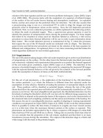
environment at 30ºC/40%RH. Fig. 7 shows the measured skin temperature data of Stolwijk
and Hardy (1966) and the simulation results of Zolfaghari and Maerefat (2010) for STB and
Pennes bioheat models. It can be clearly seen that the Pennes bioheat model is not able to
accurately estimate the skin temperature under hot environmental conditions. As shown in
Fig. 7, the Pennes bioheat model overestimates the value of the skin temperature more than
3.5ºC under the mentioned extremely hot conditions. This inaccuracy may be caused by

neglecting the thermoregulatory mechanisms such as regulatory sweating and vasomotion
in Pennes bioheat model. However, as can be seen in Fig. 7, the results of the STB model are
in a good agreement with the experimental results.

28
30
32
34
36
38
40
42
0 30 60 90 120 150 180 210
Time (min)
Skin Temperature (ºC)
Experiments (Stolwijk and Hardy, 1966)
Pennes' Model
STB Model

Fig. 7. Comparison of measured (Stolwijk & Hardy, 1966) and simulated skin temperature
(Pennes’ model and the STB model) during temperature step change
Despite the simplicity of the STB model, it is able to accurately predict the temperature in
the cutaneous layer under a wide range of personal/environmental conditions. Also,
Zolfaghari and Maerefat (2010) showed that, because of the simplicity and reasonable
accuracy of the STB model, it can be widely used in predicting the thermal response of the
human body under both transient and steady-state environments. Therefore, the STB model
can be utilized for evaluating thermal comfort of the human body in variant
personal/environmental conditions. Furthermore, the model validations show that the
model results are sufficiently reliable under extremely hot/cold conditions (Zolfaghari &
Maerefat, 2010).

Bioheat Transfer

169
5. Conclusion
In this chapter, a brief review of bioheat transfer models (e.g. Pennes’ bioheat equation,
Wulff Continuum Model, Klinger Continuum Model, Chen-Holmes model, Weinbaum-Jiji-
Lemons vascular model and simplified Weinbaum-Jiji vascular Model) has been presented.
Also, a new simplified thermoregulatory bioheat (STB) model (Zolfaghari & Maerefat, 2010)
has been briefly introduced in the present chapter. The STB model has been developed by
combining the well-known Pennes’ equation with Gagge’s two-node model for evaluating
the temperature in the cutaneous layer under a wide range of personal/environmental
conditions. This model considers the effects of thermoregulatory mechanisms of the human
body by defining the thermal control signals of the body. The STB model has been validated
against the published experimental and analytical results, where a good agreement has been
found (Zolfaghari & Maerefat, 2010). Therefore, the results of the STB model are sufficiently
reliable for estimating the cutaneous themperature under both transient and steady-state
thermal conditions.
6. References
Chato, J.C. (1980). Heat Transfer to Blood Vessels, ASME Journal of Biomechanical Engineering,
Vol. 102, pp. 110-118, ISSN 0148-0731
Chen, M.M. & Holmes, K. R. (1980). Microvascular Contributions in Tissue Heat Transfer,
Annals of the New York Academy of Sciences, Vol. 335, pp. 137–150, ISSN 0077-8923
Cho, Y.I. (1992). Bioengineering Heat Transfer, In: Advances in Heat Transfer, J.P. Hartnett &
T.F. Irvine, (Ed.), Academic Press, Inc., ISBN 978-0-12-020022-8, San Diego, USA
Campbell, I. (2008). Body Temperature and its Regulation. Anaesthesia & Intensive Care
Medicine, Vol. 9, No. 6, pp. 259-263, ISSN 1472-0299
Datta, A.K. (2002). Biological and Bioenvironmental Heat and Mass Transfer, Marcel Dekker,
Inc., ISBN 978-0-8247-0775-3, New York, USA
Doherty, T. & Arens, E.A. (1988). Evaluation of the Physiological Bases of Thermal Comfort

Models. ASHRAE Transaction, Vol. 94, pp. 1371-1385, ISSN 0001-2505
DuBois D. & DuBois E.F. (1916) A Formula to Estimate Approximate Surface Area, if Height
and Weight are Known. Archives of Internal Medicine, Vol. 17, pp. 863-871, ISSN
0003-9926
Fanger P.O. (1970). Thermal Comfort Analysis and Applications in Environmental Engineering,
McGraw-Hill, ISBN 0-07-019915-9, New York, USA
Jiji, L.M. (2009). Heat Conduction, Third Edition, Springer, ISBN 978-3-642-01266-2, Berlin,
Germany
Kaynakli O. & Kilic M. (2005). Investigation of indoor thermal comfort under transient
conditions. Building and Environment, Vol. 40, No. 2, pp. 165-174, ISSN 0360-1323
Klinger, H.G. (1974). Heat transfer in perfused biological tissue. I. General theory. Bulletin of
Mathematical Biology, Vol. 36, pp. 403-415, ISSN 1522-9602
Kreith, F. (2000). The CRC Handbook of Thermal Engineering, CRC Press, ISBN 978-0-8493-
9581-9, Boca Raton, USA
Kutz, M. (2009). Biomedical Engineering and Design Handbook, Second Edition, McGraw-Hill,
ISBN 978-0-07-170472-4, New York, USA
Lv Y.G. & Liu J. (2007). Effect of transient temperature on thermoreceptor response and
thermal sensation. Building and Environment, Vol. 42, pp. 656-64, ISSN 0360-1323

Developments in Heat Transfer

170
Minkowycz, W.J., Sparrow, E.M. & Abraham, J.P. (2009). Advances in Numerical Heat Transfer:
Volume 3, CRC Press, ISBN 978-1-4200-9521-0, Boca Raton, USA
Pennes, H.H. (1948). Analysis of Tissue and Arterial Blood Temperatures in the Resting
Forearm, Journal of Applied Physiology, Vol. 1, pp. 93-122, ISSN 1522-1601
Raaymakers, B.W., Kotte, A.N.T.J. & Lagendijk, J.J.W. (2009). Discrete Vasculature (DIVA)
Model Simulating the Thermal Impact of Individual Blood Vessels for In Vivo Heat
Transfer, In: Advances in Numerical Heat Transfer: Volume 3, Minkowycz, W.J.,
Sparrow, E.M. & Abraham, J.P., pp. 121-148, CRC Press, ISBN 978-1-4200-9521-0,

Boca Raton, USA
Sharma, K.R. (2010). Transport Phenomena in Biomedical Engineering, McGraw-Hill, ISBN 978-
0-07-166398-4, New York, USA
Stolwijk J.A.J. & Hardy J.D. (1966). Temperature regulation in man — A theoretical study.
Pflügers Archiv European Journal of Physiology, Vol. 291, No. 2, pp. 129-62, ISSN 0031-
6768
Vafai, K. (2011). Porous Media: Applications in Biological Systems and Biotechnology, CRC Press,
ISBN 978-1-4200-6541-1, Boca Raton, USA
Wan, X. & Fan, J. (2008). A Transient Thermal Model of the Human Body-Clothing-
Environment System. Journal of Thermal Biology, Vol. 33, pp. 87-97, ISSN 0306-4565
Weinbaum, S., Jiji, L.M. & Lemons, D.E. (1984). Theory and experiment for the effect of
vascular microstructure on surface tissue heat transfer. Part I. Anatomical
foundation and model conceptualization. ASME Journal of Biomechanical
Engineering, Vol. 106, pp. 321-330, ISSN 0148-0731
Weinbaum, S. & Jiji, L.M. (1985). A new simplified bioheat equation for the effect of blood
flow on local average tissue temperature. ASME Journal of Biomechanical
Engineering, Vol. 107, pp. 131-139, ISSN 0148-0731
Wulff, W. (1974). The Energy Conservation Equation for Living Tissues. IEEE Transactions-
Biomedical Engineering, vol. 21, pp. 494-495, ISSN 0018-9294
Yigit, A. (1999). Combining Thermal Comfort Models. ASHRAE Transactions, Vol. 105, pp.
149-158, ISSN 0001-2505
Zolfaghari, A. & Maerefat, M. (2010). A New Simplified Thermoregulatory Bioheat Model
for Evaluating Thermal Response of the Human Body to Transient Environment.
Building and Environment, Vol. 45, No. 10, pp. 2068-2076, ISSN 0360-1323
10
The Manufacture of Microencapsulated
Thermal Energy Storage Compounds
Suitable for Smart Textile
Salaün Fabien
1,2

1
Univ Lille Nord de France,
2
ENSAIT, GEMTEX;
France

1. Introduction
Smart textiles are able to sense electrical, thermal, chemical, magnetic, or other stimuli from
the environment and adapt or respond to them, using functionalities integrated into the
textile structure. As an important consideration in active wear, clothing comfort is closely
related to microclimate temperature and humidity between clothing and skin.
Since the end of the 80’s, functional textiles have been developed to enhance textile
performances according to the consumers’ demand and to include a large range of
properties with a higher added value. One of the possible ways to manufacture functional
or intelligent textile products is the incorporation of microcapsules or the use of
microencapsulation processes for textile finishing. Thermal storage by latent heat was early
recognised as an attractive alternative to sensible heat storage to improve the thermal
performance of clothing during the modifications of environmental temperature conditions.
Early efforts in the development of latent heat storage used organic phase change materials
(PCMs) for this purpose. PCMs are entrapped in a microcapsule of a few micrometers in
diameter to protect them and to prevent their leakage during its liquid phase. In the two
past decades, microencapsulated Phase Change Materials have drawn an increasing interest
to provide enhanced thermal functionalities in a wide variety of applications. When the
encapsulated PCMs is heated above its phase change temperature, it absorbs heat as it goes
from a solid state to a liquid state or during a solid to solid transition. It can be applied to
clothes technology, building insulation, energy storage as well as to coolant liquids. On a
more general basis, it can be used to design a broad variety of thermal transient regimes.
Recent research has investigated the incorporation of organic PCMs directly into the fabric
fibers (Zhang et al. (2006)) or coated on the substrate surface (Choi et al. (2004), Shin et al.
(2005)), creating functional and effective textile elements which can significantly affect

thermal insulation. Moreover, thermal comfort sensation is closely related to microclimate
temperature and humidity. Thus, Fan & Cheng (2005) denoted that a lower moisture
absorption rate is beneficial to thermal comfort. Therefore, the thermal functional
performance of a thermoregulated fabric is not only influenced by the latent heat of PCMs
but also by the design of the textile structure.

Developments in Heat Transfer

172
2. Classification of heat storage materials to melting temperature range and
textile application
Among the various heat storage technologies available, i.e. sensible heat based on increasing
the temperature without changing the phase of the material, latent heat based on the
transition of a material according to the temperature and thermo-chemical heat (or heat of
reaction) based on the thermophysics of the reactions; thermal heat storage in the form of
latent heat of phase change seems to be particularly attractive in textile fields. A variety of
PCMs are well-known for their thermal characteristics relating to their phase change stage.
These compounds possess the ability to absorb and store large amounts of latent heat during
the heating process and release this energy during the cooling process. Thus, materials being
converted from solid to liquid, from liquid to solid or solid 1 to solid 2 states are suitable to
be used in the manufacture of thermoregulated textiles. The selection of a PCMs formulation
depends typically on the required phase change temperature depending on end use. Indeed,
PCMs should react to changes in temperature of both the body and the outer layer of the
garment when they are incorporated in the textile substrate. Thus, for textile applications,
PCMs with a phase change within the ambient temperature and comfort range of humans
are suitable, i.e. in a temperature range from 15°C to 35°C.
Among the various ways to store energy, the most attractive form is latent heat storage in
phase change material, because of the advantages of high storage capacity in a small volume
and charging/discharging heat from the system at a nearly constant temperature (Abhat,
1983). Thermal storage by latent heat was recognised early as an attractive alternative to

sensible heat storage to improve the thermal performance of clothing during the changes of
environmental temperature conditions. The latent heat associated with a first-order phase
transition provides a mechanism for the thermal energy storage. The phase changes
comprise predominantly solid-liquid transitions for thermal storage applications in textiles.
The use of PCMs is linked to its latent heat of fusion for thermal storage. The latent heat of
fusion of a material is substantially greater than its sensible heat capacity. Stated differently,
the amount of energy that a material absorbs upon melting or releases upon freezing is
much greater than the amount of energy which it absorbs with a weak variation of
temperature. Upon melting or freezing, a PCM absorbs and releases substantially more
energy than a sensible heat storage material which is heated or cooled to the same
temperature range. The storage capacity of PCMs (Q) equals the phase change and the
sensible heat stored at the phase change temperature (1). Thus, the latent storage is always
increased by a significant extent by their sensible storage capacity. Furthermore, during the
complete phase change process, the temperature of the PCMs as well as the surrounding
media remains nearly constant (Feldman et al., 1986).

end
Tr
initial Tr
T
T
pp
TT
Q = m. C(T).dT m.H m. C(T).dT+Δ+
∫∫
(1)
For a textile application, the following PCMs properties should be required, i.e. a high value
of the heat of fusion and specific heat per unit volume and weight; a melting point in the
application range (between 15°C to 35°C); a high thermal conductivity; a chemical stability
and non-corrosiveness; PCMs should not be hazardous, non-flammable or poisonous; PCMs

should have a reproducible crystallisation without decomposition; PCMs should present a
small supercooling degree and high rate of crystal growth; they should have a small volume
The Manufacture of Microencapsulated
Thermal Energy Storage Compounds Suitable for Smart Textile

173
variation during the phase change process; and PCMs should be sufficiently abundant at a
low cost.
The most common PCMs, with a phase change temperature suitable for textile application,
can be divided into two groups, i.e. organic compounds such as paraffins or linear alkyl
hydrocarbon and non paraffinic materials (hydrocarbon alcohol, hydrocarbon acid,
polyethylene or polytetramethylene glycol, aliphatic polyester…), and inorganic compounds
such as hydrated inorganic salts, eutectics or polyhydric alcohol-water solution (Zhang,
2001).


Fig. 1. Temperature ranges and corresponding melting enthalpy of suitable PCMs for textile
applications
2.1 Organic phase change materials
Organic solid–liquid PCMs include paraffin, alkyl esters and acids, polyethylene glycol and
its derivatives.
2.1.1 Polyhydric alcohols
Polyhydric alcohol, or plastic crystal, are solid-solid phase change materials, and even if
they are not suitable for textile application since their phase change temperature is higher
than the upper end-use limit, they present small volume change, lower undercooling, no
phase separation and no leakage. Amongst them, pentaerythritol (C(CH
2
OH)
4
), trimethylol

ethane ((CH
3
)C(CH
2
OH)
3
), neopentyl glycol ((CH
3
)
2
C(CH
2
OH)
2
), their NH
2
-substituted
compounds and 2-amino-2-methyl-1,3-propanediol ((CH
2
CH
2
OH)
2
CCH
3
NH
2
), 2-amino-2-
hydroxymethyl-1,3-propanediol ((CH
2

CH
2
OH)
3
CNH
2
), and their binary mixtures have an
endothermic or exothermic effect under their melting point and are cited as potential
candidate for thermal energy storage. Furthermore, the phase change temperatures and heat