Developments in Heat Transfer Part 3 docx

Developments in Heat Transfer


70
6.1 Effect of axial magnetic field on convective heat transfer
In case of flow of liquid metals in heated channels under the influence of a uniform axial
magnetic field shows a decrease of convective heat transfer at low and moderate Hartmann
numbers whereas the convective heat transfer and hence Nu increases at higher Hartmann
numbers as shown in Miyazaki (1988). It was stated in section 4 that an axial magnetic field
does not affect the mean velocity distribution so the modification of convective heat transfer
is due the variation in the turbulent fluctuations in time and space.

Reynolds number Hartmann Number
=0
Nu/Nu
B

3
(2.5 5) 10
−
⋅

360 0.83
4
(1 2) 10−⋅
700 0.50
4
(3 4) 10−⋅
1400 0.30

4
110⋅
3600 2.75
Table 2. Variation of Nusselt Number with Axial Magnetic Field, Miyazaki (1988)
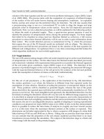
The values of Nu for various value of Hartmann numbers is shown in table 2. It can be seen
that the values of Nu decreases from its value,
=0
Nu/Nu
B
= 1, at Ha = 0. The decrease in Nu
value for small and moderate Ha is more when the Reynolds number is high because of the
higher turbulence content in the flow. At lower values of Reynolds numbers, the flow will
be inherently laminar and therefore the reduction in Nu due to suppression of turbulent
fluctuations will be low.
At high values of Hartmann numbers, the Nusselt number was found to increase, violating
the earlier theories and studies, see Miyazaki (1988). Miyazaki attributes the increase in the
Nusselt number is due to the increase in turbulence levels in the flow as the effect of
buoyancy can be ruled out because the flow direction upwards.
6.2 Effect of transverse magnetic field on convective heat transfer
The studies in the field of effect of magnetic field on convective heat transfer in ducts
subjected to transverse magnetic field can be classified into two cases
1.
Absence of high velocity jets near the side walls
2.
Presence of high velocity jets near the side walls
6.2.1 Case 1: Absence of high velocity jets near the side walls
In case of ducts having Hartmann walls with zero conductivity, high velocity jets will not be
formed near the side walls. Gardener and Lykoudis (1971b) performed experiments with
flow of Mercury in horizontal electrically insulated pipe subjected to transverse magnetic
field. It was found that the velocity profile near the Hartmann wall becomes flat with

increase in magnetic field as discussed in section 4.1 and the velocity profile near side walls
becomes round as discussed in sections 4.2.1 and 4.2.2. The mean velocity distribution is not
much different with the increase in magnetic field, so the modification of turbulence
phenomenon by the magnetic field will affect the convective heat transfer predominantly for
this case. The Nusselt number distribution near the Hartmann and side walls for a range of
Reynolds numbers and Hartmann numbers is shown in figure 12. The decrease of Nusselt
number with increase in magnetic field is lesser at lower Reynolds number because the
turbulence content in the flow at low Reynolds number will be lesser.

Magneto Hydro-Dynamics and Heat Transfer in Liquid Metal Flows


71
0
10
20
30
40
10000 100000 1000000
Nu
No magnetic field
Hartmann wall - Ha 375
Side wall - Ha 375
10
4
10
5
10
6
1

10
20
30
40
No magnetic field
Hartmann – Ha 375
Side – Ha 375
Re
Nu
0
10
20
30
40
10000 100000 1000000
Nu
No magnetic field
Hartmann wall - Ha 375
Side wall - Ha 375
10
4
10
5
10
6
1
10
20
30
40

No magnetic field
Hartmann – Ha 375
Side – Ha 375
Re
Nu

Fig. 12. Nusselt number with magnetic field intensity, Gardener and Lykoudis (1971b)
The reduction in Nusselt number with increase in magnetic field is because of the reduction
in turbulence quantified using turbulence kinetic energy as shown in figure 13. It was found
that the turbulent kinetic energy decreases both near the Hartmann and side walls with
increase in magnetic field where r/R = 0 represents the centre of the duct and r/R = 1
represents the walls. The damping force within the Hartmann layer is much higher than at
the side region due to the high local electric current density. The turbulence in core is
suppressed initially and then the turbulence in the Hartmann layer followed by the
turbulence near the side wall.

0
5000
10000
15000
20000
25000
30000
35000
0.00 0.20 0.40 0.60 0.80 1.00
r/R
Turbulent Kinetic Energy
m
2
/s

2
No magnetic field
Hartmann wall - Ha 47
Side wall - Ha 47
0.5
1.0
1.5
2.0
2.5
3.0
3.5
0.0
Turbulent Kinetic Energy
x 10
4
m
2
/s
2
0
5000
10000
15000
20000
25000
30000
35000
0.00 0.20 0.40 0.60 0.80 1.00
r/R
Turbulent Kinetic Energy

m
2
/s
2
No magnetic field
Hartmann wall - Ha 47
Side wall - Ha 47
0.5
1.0
1.5
2.0
2.5
3.0
3.5
0.0
Turbulent Kinetic Energy
x 10
4
m
2
/s
2

Fig. 13. Turbulent kinetic energy vs. r/R for Re = 50,000, Gardener and Lykoudis (1971a)
A correlation for Nusselt number values is created from various experimental results by Ji
and Gardener (1997) and is given using the following relation as a function of Peclet number
Pe and Hartmann number Ha

()
()

0.811
1.5
0.00782Pe
Nu 7
1 0.0004Ha Pef
=+
+
(27)
()
(
)
592
Pe 0.3 4.75 10 Pe 2.10 10 Pef
−−
=+× −×

Developments in Heat Transfer


72
6.2.2 Case 2: Presence of high velocity jets near the side walls
In case of ducts having Hartmann walls with finite conductivity, high velocity jets will be
formed near the side walls. The side layers with high velocity jets (M shaped profile, figure 8
case 3) carry high mass flux is the prime reason for increase of heat transfer near the side
walls. Miyazaki et al. (1986) performed experiments to determine the heat transfer
characteristics for liquid metal Lithium flow in annular duct with electrically conducting
walls under the influence of transverse magnetic fields. The Nusselt number plotted with
magnetic field is shown in figure 14. It can be seen that the Nusselt number increases near
the side walls and decreases near the Hartmann walls. A singular rise of Nusselt number
can be seen near both the walls.

5.0
5.5
6.0
6.5
7.0
7.5
8.0
8.5
0.00 0.20 0.40 0.60 0.80 1.00
Magnetic FIeld, Tesla
Nu
Side Walls
Hartmann Walls

Fig. 14. Nusselt number plotted with magnetic field intensity, Miyazaki (1986)
This effect of heat transfer enhancement near the side walls is caused by the generation and
development of large scale velocity fluctuations in the near wall area. The reduction in
Nusselt number near the Hartmann walls is created due to the turbulence reduction as
shown in figure 15.

0.0
0.2
0.4
0.6
0.8
0.00 0.20 0.40 0.60 0.80 1.00
Magnetic FIeld, Tesla
Side Walls
Hartmann Walls

RMS of Temperature
Fluctuation (
0
C)
0.0
0.2
0.4
0.6
0.8
0.00 0.20 0.40 0.60 0.80 1.00
Magnetic FIeld, Tesla
Side Walls
Hartmann Walls
RMS of Temperature
Fluctuation (
0
C)

Fig. 15. RMS of temperature fluctuation with magnetic field intensity, Miyazaki (1986)

Magneto Hydro-Dynamics and Heat Transfer in Liquid Metal Flows


73
7. Application of numerical codes
A difficulty in experimental study of the flow of liquid metals arises as the visualization is
not possible because of the opaque nature of liquid metals. Application of closed form
analytical solutions is limited to simple cases where the equations are not very complex.
This makes the application of numerical simulations useful for the study of liquid metal
magneto-hydro-dynamic flows. An example of application of a numerical code to explain

the mechanisms affecting heat transfer for flow subjected to transverse magnetic field is
explained using a series of simulations given in Rao and Sankar (2010), see figure 16.

x
y
300
T
4
T
5
T
7
T
8
B
30
7.6
15.8
1.65
1.1
Heater Pin
Flow
Direction
Fluid Elements
Solid Elements
(a)
(b)
Height of the first
cell = 1μm
x

y
300
T
4
T
5
T
7
T
8
B
30
7.6
15.8
1.65
1.1
Heater Pin
Flow
Direction
Fluid Elements
Solid Elements
(a)
(b)
Height of the first
cell = 1μm

Fig. 16. (a) Schematic of model (b) Details of the computational mesh, Rao and Sankar (2010)
A numerical study is conducted in an annular duct formed by a SS316 circular tube with
electrically conducting walls and a coaxial heater pin, with liquid Lithium as the working
fluid for magnetic field ranging from 0 – 1 Tesla The Hartmann and Stuart number of the

study ranges from 0 – 700 and 0 – 50 respectively. The Reynolds number of the study is 10
4
.
It was shown that the convective heat transfer and hence the Nusselt number decreases near
the walls perpendicular to the magnetic field due to reduction in turbulent fluctuations with
increase of magnetic field. It was observed that the Nusselt number value increases near the
walls parallel to the magnetic field as the mean velocity increases near the walls. A singular
rise was observed near both the walls near Stuart number ~ 10 which is due to the increase
of turbulence levels in the process of changing from turbulent to electromagnetically
laminarized flow, see figure 17.
When a very low Reynolds number ~ 300 is used, the reduction in Nusselt number near the
Hartmann walls is less as shown in figure 18. This shows that the reduction in Nusselt
number near the Hartmann walls for the high Reynolds number study is due to the
reduction in turbulent fluctuations. The Nusselt number was found to increase near the side
walls as the mean velocity increases near the walls. When an insulating duct is used the
Nusselt number near the parallel walls did not increase for the case with insulating walls as

Developments in Heat Transfer


74
in the case with conducting walls showing the contribution of the ‘M’ shaped velocity
profile in the Nusselt number increase near the parallel walls. The Nusselt number near the
perpendicular walls was found to decrease at a higher rate in case of insulating walls than
that of the study with conducting walls as shown in figure 19.

0.6
0.8
1.0
1.2

1.4
0.0 0.2 0.4 0.6 0.8 1.0
Hartmann wall
Side wall
Nu/Nu
B=0
0.0
1.7
7.5
16.9
30.1
47.0
Tesla
St
0.0
0.2
0.4
0.6
0.8
1.0
0.6
0.8
1.0
1.2
1.4
Hartmann wall
Side wall
0.6
0.8
1.0

1.2
1.4
0.0 0.2 0.4 0.6 0.8 1.0
Hartmann wall
Side wall
Nu/Nu
B=0
0.0
1.7
7.5
16.9
30.1
47.0
Tesla
St
0.0
0.2
0.4
0.6
0.8
1.0
0.6
0.8
1.0
1.2
1.4
Hartmann wall
Side wall

Fig. 17. High Reynolds number with conducting walls, Rao and Sankar (2010)

Nu/Nu
B=0
0.8
1.0
1.2
1.4
1.6
0.0 0.2 0.4 0.6 0.8
Hartmann wall
Side wall
Nu/Nu
B=0
0.00
1.78
7.52
16.93
30.10
Tesla
St
0.0
0.2
0.4
0.5
0.8
0.8
1.0
1.2
1.4
1.6

Hartmann wall
Side wall
Nu/Nu
B=0
0.8
1.0
1.2
1.4
1.6
0.0 0.2 0.4 0.6 0.8
Hartmann wall
Side wall
Nu/Nu
B=0
0.00
1.78
7.52
16.93
30.10
Tesla
St
0.0
0.2
0.4
0.5
0.8
0.8
1.0
1.2
1.4

1.6
Hartmann wall
Side wall

Fig. 18. Low Reynolds number with conducting walls, Rao and Sankar (2010)

0.70
0.75
0.80
0.85
0.90
0.95
1.00
1.05
0.00 0.20 0.40 0.60 0.80 1.00
Side wall
Hartmann wall
Nu/Nu
B=0
0.00
1.78
7.52
16.93
30.10
47.04
Tesla
St
0.00
0.2
0.4

0.6
0.8
1.0
0.70
0.75
0.80
0.85
0.90
0.95
1.00
1.05
Hartmann wall
Side wall
0.70
0.75
0.80
0.85
0.90
0.95
1.00
1.05
0.00 0.20 0.40 0.60 0.80 1.00
Side wall
Hartmann wall
Nu/Nu
B=0
0.00
1.78
7.52
16.93

30.10
47.04
Tesla
St
0.00
0.2
0.4
0.6
0.8
1.0
0.70
0.75
0.80
0.85
0.90
0.95
1.00
1.05
Hartmann wall
Side wall

Fig. 19. High Reynolds number with insulating walls, Rao and Sankar (2010)

Magneto Hydro-Dynamics and Heat Transfer in Liquid Metal Flows


75
8. Application of liquid metal MHD studies in nuclear fusion reactors
International Thermo-nuclear Experimental Reactor is an international organization formed
in 1985 comprising of researchers from US, EU, China, Japan, India, Korea and Russia

working towards development of a test reactor (TOKOMAK) which is expected to be
developed by 2020. The test reactor will be installed in France where the head office of ITER
is situated. Salient details of the reactor to be developed are shown in figure 20. The reactor
height will be close to 100 ft and would weigh around 38000 tons. The cryostat is the
external chamber around the TOKOMK which maintains high vacuum inside it to reduce
the heat load from atmosphere through conduction and convection. The fusion of Deuterium
and Tritium happens inside the plasma chamber. The magnets are used to confine the
plasma created inside the plasma chamber using a magnetic field of 4-8 Tesla.

Plasma
Chamber
Cryostat
Central
Solenoid
Toroidal
Magnets
Plasma
Chamber
Cryostat
Central
Solenoid
Toroidal
Magnets

Fig. 20. Details of the TOKOMAK
Tritium breeding modules are used in fusion reactors to produce Tritium by reacting
Lithium with neutrons a byproduct of the nuclear fusion reaction. The two basic breeder
concepts developed by ITER are liquid breeder and solid breeders. The advantages of liquid
breeder over solid breeder are the high Tritium breeding ratio and the Lead-Lithium
eutectic can also act as a coolant inside the breeding module which is subjected to high heat

Developments in Heat Transfer


76
from plasma and the heat generated in itself due to bombardment of neutrons. The major
disadvantages of liquid breeders over solid breeders is the pressure drop in the form of
Lorentz force and the reduction in convective heat transfer characteristics of the liquid metal
when it is flowing in the presence of intense magnetic field produced by the cryogenic
super-conducting magnets.
Wong et al. (2008) has mentioned about the various liquid metal breeders being developed
around the world details of which is given in the table 3. All the liquid breeder design uses
Lithium as the breeding material though most of them use a eutectic of Lead and Lithium
because of the lower electrical conductivity and the neutron multiplication ability of Lead.

Country Name of TBM Liquid Metal Used
US DCLL – Dual Coolant Lead Lithium PbLi
EU HCLL – Helium Cooled Lithium Lead PbLi
Korea HCML – Helium Cooled Molten Lithium Li
India LLCB - Lead-Lithium Cooled Ceramic Breeder PbLi
China DFLL – Dual Functional Lithium Lead PbLi
Table 3. Details of the liquid TBM developed in the various countries, Wong et al. (2008)

First
Wall
Pb-Li Inlet
Poloidal View Exploded View
PbLi
First
Wall

Pb-Li Inlet
Poloidal View Exploded View
PbLi
First
Wall
Pb-Li Inlet
Poloidal View Exploded View
PbLi

Fig. 21. Details of LLCB- TBM, Wong et al. (2008)

Magneto Hydro-Dynamics and Heat Transfer in Liquid Metal Flows


77
Indian Lead lithium Cooled Ceramic Breeder (LLCB) – The design description of LLCB is given
in Rao et al. (2008). The details of the exploded and cut section views of the LLCB – TBM is
shown in figure 21. The two coolants used in LLCB are Helium and a eutectic of Lead-
Lithium, Pb-Li. The two coolants are of different molecular properties as Pb-Li has very low
Prandtl Number of the order 10
-2
and Helium gas has Prandtl number of ~0.65. The thermal
diffusivity of the two fluids were different as the main temperature difference for Helium in
straight ducts were concentrated at the viscous sub layer where as the temperature
difference for Pb-Li was also present in the mean core region.
The material of construction of the cooling channels is Ferritic-Martensitic Steel (FMS)
having electrical conductivity of the order 10
6
1/Ώ-m, so the pressure drop associated with
the flow was very high. Hence a coating of Alumina (Al

2
O
3
), which has very low electrical
conductivity (~10
-8
1/ Ώ-m) is used on the wet surfaces of the cooling channels This makes
the configuration similar to the rectangular channel of Shercliff’s case with all walls
insulating i.e. d
A
= 0 and d
B
= 0 and hence as mentioned in 4.2.1, the velocity profiles will not
have a high velocity jet near the side walls. So the effect of turbulence modification is more
significant on the heat transfer characteristics as mentioned in section 6.2.1. The flow will be
electromagnetically laminarized and the heat transfer capacity of the Pb-Li deteriorates at
high Hartmann numbers.
9. Nomenclature
2a Distance between Hartmann walls
2b Distance between side walls
B
0
Magnetic field
c Speed of light
C
p
Specific heat
d
A
Electrical conductivity of wall AA

d
B
Electrical conductivity of wall BB
D Displacement current
E Electric field
H Magnetic field strength
Ha Hartmann Number
j Electric charge
k Thermal conductivity
k
eff
Effective thermal conductivity
k
Τ
Turbulent thermal conductivity
L Characteristic length
N Interaction parameter
Nu Nusselt number
p Pressure
Pr Prandtl number
Pr
m
Magnetic Prandtl number
q
'''
Volumetric heat generation
S Source term
Re Reynolds number

Developments in Heat Transfer

78
Re
m
Magnetic Reynolds number
t Time
T Temperature
U Axial velocity
U
c
Centre line velocity
U
0
Mean velocity

σ
Electrical conductivity of fluid
η
Non-dimensionalized distance in y direction
ξ
Non-dimensionalized distance in x direction
ν
Kinematic viscosity of fluid
eff
ν
Effective viscosity
τ
ν
Turbulent viscosity

ρ
Density of fluid
μ
Dynamic viscosity of fluid
*
μ
Magnetic permeability
c
ρ
Electric charge density

10. Acknowledgement
We would like to acknowledge Altair Engineering India Pvt. Ltd., for providing an
opportunity to do the associated work

11. References
Alfven, H. (1942). Existence of electromagnetic-hydrodynamic waves. Nature, Vol.150,
(1942), pp.405-406.
Davidson, H. W. (1968). Compilation of thermo-physical properties of liquid Lithium NASA
Technical Note, Washington. D. C., 1968.
Evtushenko, I. A.; Hua, T. Q.; Kirillov. I. R.; Reed, C. B. & Sidorenkov, S. S. (1995). The effect
of a magnetic field on heat transfer in a slotted channel. Journal of Fusion Engineering
and Design, Vol. 27, (1995), pp. 587-592.
Fink, D. & Beaty, H. W. (October 1999). Standard handbook for electrical engineers (14
th
Edition).
McGraw Hill, ISBN 0070220050.
Gardener, R. A. & Lykoudis, P. S. (1971a). Magneto-fluid-mechanic pipe flow in a transverse
magnetic field Part 1 Isothermal flow. Journal of Fluid Mechanics, Vol.47, (1971), pp
737-764.

Gardener, R. A. & Lykoudis, P. S. (1971b). Magneto-fluid-mechanic pipe flow in a transverse
magnetic field Part 1 Heat Transfer. Journal of Fluid Mechanics, Vol.48, (1971), pp.
129-141.
Happel, J. & Brenner, H. (1981). Low Reynolds Number Hydrodynamics, Springer. ISBN
9001371159.

Magneto Hydro-Dynamics and Heat Transfer in Liquid Metal Flows


79
Hartmann, J. (1937) Theory of the laminar flow of electrically conductive liquid in a
homogeneous magnetic field, Hg-Dynamics, Kgl. Danske Videnskab. Selskab. Mat
fus. Medd., Vol.15, No.6, (1937)
Hartmann, J. & Lazarus. P. (1937). Experimental investigation of flow of Mercury in a
homogeneous magnetic field, Kgl. Damske Videnskabernes Selskab, Math-,Fys. Med,
Vol.14, No. 7, (1937).
Hunt, J. C. R. (1965). Magnetohydrodynamic flow in rectangular ducts. Journal of fluid
mechanics, Vol. 21, No. 4, (1965), pp. 577-590.
Hunt, J. C. R. & Stewartson, K. (1965). Magnetohydrodynamic flow in rectangular ducts. II.
Journal of fluid mechanics, Vol. 23, No.3, (1965), pp. 563-581.
Ji, H. C. & Gardener, R. A. (1997). Numerical analysis of turbulent pipe flow in a transverse
magnetic field. International Journal of Heat and Mass Transfer, Vol.40, No.8, (1997),
pp. 1839-1851.
Kirillov, I. R.; Reed, C. B.; Barleon, L. & Miyazaki, K. (1994). Present understanding of MHD
and heat transfer phenomenon for liquid metal blankets, Proceedings of 3rd
International Symposium of Fusion Nuclear Technology, Los Angeles, 1994.
Lielpeteris, J & Moreau, R. (1989). Liquid metal magnetohydrodynamics, Kluwer Academic
Publishers Group, ISBN 079230344X, Dordrecht, Boston.
Luo, X.; Ying, A. & Abodu, M. (2003). Experimental and computational simulation of free jet
characteristics under transverse field gradients. Journal of Fusion Science and

Technology, Vol 44, (July 2003), pp. 85-93.
Miyazaki, K.; Inoue, h.; Kimoto, T. ; Yamashita, S.; Inoue, S. & Yamaoka, N. (1986).
Heat transfer and temperature fluctuation of lithium flowing under transverse
magnetic field. Journal of Nuclear Science and Technology, Vol.23, (1986), pp. 582-
593.
Miyazaki, K.; Yokomizo, K.; Nakano, M.; Horiba, T. & Inoue, S. et al. (1988). Heat Transfer
and Pressure Drop of Lithium Flow under Longitudinal Strong Magnetic Field,
Proceedings of LIMET’88, Avignon, 1988.
Moffatt, H. K. (1967). On the suppression of turbulence by a uniform magnetic field. Journal
of Fluid Mechanics, Vol. 28, (1967), pp. 571–592.
Muller, U. & Buhler, H. (2001), Magneto-fluid-dynamics in Channels and Containers (1
st

Edition), Springer, ISBN 978-3-540-41253-3.
Rao, J. S. et al.(2008). Design description document for the dual coolant Pb 17Li (DCLL) test blanket
module, Report to the ITER test blanket working group (TBWG), (2008), Institute of
Plasma Research, India.
Rao, J. S. & Sankar, H. (2011). Numerical Simulation of MHD Effects on Convective Heat
Transfer Characteristics of Flow of Liquid Metal in Annular Tube. Journal of Fusion
Engineering and Design, Vol.86, No.2-3, (March 2011), pp. 183-191.
Roberts, P. H. (1967). An Introduction to Magnetohydrodynamics, Longmans Green and Co Ltd,
1967, ISBN 978-0-582-44728-8.
Shercliff, J. A. (1953). Steady motion of conducting fluids in pipes under transverse magnetic
fields, Proceedings of Cambridge Philosophical Society, pp. 136-144, 1953.
Uda, N.; Miyazawa, A. ; Inoue, S.; Yamaoka, n.; Horiike, H. & Miyazaki, k. (2001). Forced
convection heat transfer and temperature fluctuations of lithium under

Developments in Heat Transfer

80
transverse magnetic field. Journal of Nuclear Science and Technology, Vol. 38, (2001),
pp. 936-943.
Uda, N.; Miyazawa, A.; Yamaoka, H. N.; Horiike, H. & Miyazaki, K. (2002). Heat transfer
enhancement in lithium annular flow under transverse magnetic field. Energy
Conversion and Management, Vol.43, (2002), pp. 441-447.
Wong, C. P. C. ; Salavy, J. F.; Kim, Y.; Kirillov, I.; Kumar, E. R.; Morley, n. B.; Tanaka, S. &
Wu, Y. C. (2008). Overview of liquid metal TBM concepts and programs. Journal of
Fusion Engineering and Design, Vol.83, (2008), pp. 850-857.
5
Thermal Anomaly and Strength of
Atotsugawa Fault, Central Japan,
Inferred from Fission-Track Thermochronology
Ryuji Yamada
1
and Kazuo Mizoguchi
2

1
National Research Institute for Earth Science and Disaster Prevention
2
Central Research Institute of Electric Power Industry
Japan

1. Introduction
Frictional slip induces temperature rise in a fault zone. Abundant frictional heat during an
earthquake sometimes produces melt of rocks (i.e. pseudotachylyte; e.g., Sibson, 1975). The
amount of heat production along faults provides the essential information to investigate
frictional strength of the faults that characterizes the earthquake generation processes.
Lachenbruch and Sass (1980) first estimated the coefficient of friction of the San Andreas

Fault to be 0.1-0.2 from the measurement of surface heat flow along the fault. Kano et al.
(2006) found a temperature rise of ~ 0.06 °C measured in a borehole drilled across the
Chelungpu fault six years after the 1999 Chi-Chi, Taiwan earthquake associated with this
fault. They found that very low coefficient of friction of 0.04-0.08 can explain the heat
anomaly along the Chelungpu fault. The above observations along the natural faults have
suggested a very low friction level compared with that of 0.6-0.8 evaluated in laboratory
rock friction experiments (Byerlee, 1978).
Fission-track (FT) thermochronology is an effective method to detect heat anomaly caused
by past faulting (e.g., Scholz et al., 1979; Camacho et al., 2001; Murakami et al., 2002;
Murakami and Tagami, 2004; Yamada et al., 2007a). In order to constrain the frictional
properties of faults, d’Alessio et al. (2003) measured apatite FT ages and lengths for samples
adjacent to and within the San Gabriel fault zone that is thought to be an abandoned major
trace of the San Andreas Fault system active from 13 to 4 Ma. They found no evidence of a
localized thermal anomaly in FT data even in samples within just 2 cm of the
ultracataclasite, and concluded that either there has never been an earthquake with > 4 m of
slip at this locality, or the average apparent coefficient of friction is < 0.4 based on the
modelling of heat generation and transport.
In this paper, we estimate the frictional strength of the Atotsugawa fault, central Japan,
using the method similar to that used by d’Alessio et al. (2003). In the Atotsugawa fault,
Yamada et al. (2009) performed FT thermochronologic analysis at an outcrop without visible
pseudotachylyte layers, and revealed a thermal anomaly at a several cm thick gouge whose
apatite age is significantly younger than those of other samples in the vicinity. Assuming
that the thermal anomaly is cause by frictional heating during a single earthquake, the
frictional coefficient and the ancient depth of gouge samples are evaluated by the thermal

Developments in Heat Transfer

82
modelling to satisfy the constraints given by the FT thermochronological data with respect
to the geometry and alignment of the gouges in the outcrop.

2. Fission-track thermochronology in Atotsugawa fault zone
The Atotsugawa fault is a right-lateral strike-slip one with a strike of N60°E and almost
vertical dip, located in the Hida metamorphic belt, central Japan (Fig. 1). From the trenching
surveys, a number of historical large earthquakes were detected along the Atotsugawa fault;
the most recent one is the 1858 Hietsu earthquake. The estimate of the magnitude ranges 7.0
(Usami, 1987), 7.3 (Matsu'ura et al., 2006) and 7.9 (Doke and Takeuchi, 2009). Geographical
Survey Institute, Japan (GSI; 1997) reported a creeping slip with a rate of 1.5 mm/yr in the
central section of the fault.


Fig. 1. Distribution of active fault around the Atotsugawa fault. An open circle (centre) and an
open triangle (bottom left) symbols indicate the locations of an outcrop and a reference site
of R2 in Fig. 2, respectively
In the creeping section, Yamada et al. (2009) performed FT thermochronologic analysis by
measuring ages of apatite and zircon grains separated from gouges and fractured rocks at
six fracture zones within a 15 m-wide fault zone without visible pseudotachylyte layers (Fig.
2a). This fault zone consists of six fault gouges (name, thickness; gouge-1, 10 cm; gouge-2, 8-
20 cm; gouge-3, 8-25 cm; gouge-4, 10 cm; gouge-5, 10-30 cm; gouge-6, 20 cm). FT ages of
zircon (c. 120-150 Ma) and apatite (c. 44-60 Ma) for samples except "gouge-1" agree well with
emplacement ages for the Funatsu granitic rocks that intruded the Hida Belt (Matsuda et al.,
1998). The discordance in zircon and apatite FT ages is interpreted to reflect the rock cooling
due to the regional uplift and associated erosion. A thermal anomaly was identified at the
gouge sample of "gouge-1" that showed an exceptionally young apatite age (32.1 ± 3.2 Ma,
1σ) with a unimodal FT length distribution, although its zircon age (121 ± 6 Ma, 1σ) was
well concordant with other samples (Fig. 2b; after Yamada et al., 2009). The creeping slip
Thermal Anomaly and Strength of Atotsugawa Fault,
Central Japan, Inferred from Fission-Track Thermochronology

83
observed in the central section of the Atotsugawa fault (GSI, 1997) could be a possible

source for this heat anomaly. Such a low slip rate of 1.5 mm/yr, however, causes much
smaller increase in temperature (< 20 °C; d’Alessio et al., 2003) in the fault zone. This
disagreement can therefore be attributed to the secondary heating induced by frictional slip
during an associated earthquake, and the young apatite age possibly gives a younger limit
of the initiation of the activity in the Hida Belt.


Fig. 2. (a) Sketch of the outcrop of the Atotsugawa fault zone and (b) fission-track age variation
in apatite (lower) and zircon (upper) across the outcrop (after Yamada et al., 2009). Open
circle, solid circle and square symbols indicate data of fault gouge, fractured rock and host
Hida metamorphic rock, respectively. Dashed lines indicate locations of the fault gouge
zones. Two reference samples of R1 and R2 (an open triangle in Fig. 1) were also collected
where no fractures were observed. Length distribution of apatite FTs for sample ATG1G is
also shown. Shaded bands behind the plot indicate the apatite and zircon FT age distributions
of the granitic rocks that intrude into the Hida Belt (Matsuda et al. 1998). Error bars show 2σ
uncertainty in age

Developments in Heat Transfer

84
3. Thermal modelling associated with frictional heating and estimation of
frictional strength
In order to estimate the frictional strength of the Atotsugawa fault based on the FT
thermochronological data, we modelled the temporal change in the temperature in and out
of the "gouge-1" where an exceptionally young apatite age was found (Yamada et al., 2009).
The FT data and the geometry of the occurrence of gouges in the outcrop indicate that the
apatite FT age in the 10 cm thick “gouge-1” zone was thermally reset but that in the
fractured rock 10 cm apart from “gouge-1” was not. Therefore, the model space for the thermal
modelling is composed of a central slip zone of 10 cm thickness and the surrounding rock
zone of 10 m thickness with a homogeneous temperature distribution at a certain depth in

the initial state (Fig. 3). It is assumed that a single fault slip occurs at a constant rate and all
of the frictional work converts into heat. One-dimensional heat transfer model is used to
describe the heat diffusion into the surrounding zone at a direction normal to the slip zone.
The effect of thermal diffusion by fluid flow is not considered because hydraulic properties
of the Atotsugawa fault zone at depth have not yet been investigated.
The equation of thermal diffusion with frictional heat source term for the slip zone is given
by

2
2
n
rp
c
V
TT
C
tW
x
μσ
∂∂
ρκ
∂
∂
⎛⎞
⋅⋅
⋅= +
⎜⎟
⎝⎠
(1)
where T is temperature, t is the lapse time after a slip occurs, V is the slip rate of the fault, µ

is the coefficient of friction,
σ
n
is the effective normal stress on the fault, C
p
is the heat
capacity of rock, W
c
is the width of a slip zone, k is the thermal conductivity of rock,
ρ
r
is the
density of rock, and x is the distance normal to the fault from the centre of the slip zone.
The effective normal stress
σ
n
is equivalent to the effective overburden pressure given by
(
ρ
r
-
ρ
w
)·H·g, where
ρ
w
is the density of water, H is depth and g is gravity. For the surrounding
zone, Equation (1) without the heat source term (i.e., the first term in the right hand side) is
used.

Fig. 3. Fault model for thermal calculation associated with frictional heating. Distance is
measured from the centre of the fault
Thermal Anomaly and Strength of Atotsugawa Fault,
Central Japan, Inferred from Fission-Track Thermochronology

85
Table 1. Parameters used for thermal calculations
Constants of typical physical properties of rocks are used in the thermal modelling as shown
in Table 1 (c.f., Schön, 1996). W
c
is set as 10 cm that is equivalent to the thickness of the
“gouge-1”. The initial temperature at a certain depth H is obtained from a geothermal
gradient of 30 °C/km (typical value for the upper crust in Japan; e.g., Tanaka et al., 1999)
multiplied by H plus a surface temperature of 20 °C, and the temperature distribution over
the fault zone is assumed to be uniform. The boundary condition of the temperature at the
edge of the model space is fixed at the initial value. Total slip of 5 m long is given for this
fault system because the estimate of the magnitude of the associated earthquake ranges
from 7.0 to 7.9 (Usami, 1987; Matsu'ura et al., 2006; Doke and Takeuchi, 2009) that
corresponds to the total slip of the order of 1-10 m, based on the empirical relationship
between the fault displacement and the magnitude (Matsuda, 1975). V is set at 1 m/s (e.g.,
Heaton, 1990) and therefore the slip duration is 5 sec. Considering the closure temperature
of apatite FT (100 ± 20 °C; e.g., Wagner and Van den Haute 1992), H should be shallower
than 3 km which corresponds to the environment temperature of 110 °C, and therefore
restricted to the three cases of 1, 2 and 3 km for the modelling assuming a geothermal
gradient of 30°C/km (e.g., Tanaka et al, 1999).

Fig. 4. Temperatures at the centre of the fault (T
0
, solid line) and at 10 cm apart from the
centre (T

10
, dashed line) are plotted as a function of time since a slip occurs

Developments in Heat Transfer

86

(a)
(b)
Fig. 5. Maximum temperature at the centre of the fault (T
0
; a) and at the location 10 cm apart
from the centre (T
10
; b) during an earthquake are plotted as a function of friction coefficient of
0.1 ~ 0.9 in cases of depth from 1 to 3 km. Square, triangle and circle symbols denote the data
at 1, 2 and 3 km, respectively. Shaded areas in (a) and (b) indicate ranges of T
0
(upper) and
T
10
(lower) inferred from apatite and zircon FT thermochronological analyses, respectively
Calculation results of the temporal change in temperature at the two locations of x = 0 cm
(D
0
) and x = 10 cm (D
10
) for the combination of µ (0.6) and H (3 km) parameters are shown as
representative cases in Fig. 4. These locations are chosen to approximate the positions of the
"gouge-1" and a surrounding rock sample, respectively. For any combinations of µ and H

parameters, the time during which the temperature in a specific location is maintained at its
maximum is almost invariant. The temperatures at D
0
and D
10
are preserved at the
Thermal Anomaly and Strength of Atotsugawa Fault,
Central Japan, Inferred from Fission-Track Thermochronology

87
maximums of T
0
and T
10
(named T
max0
and T
max10
) for the order of ~10^2 sec and ~10^4 sec,
as indicated by shaded bands in Fig. 4, respectively. Fig. 5 shows the variations of T
max0
and
T
max10
for the combinations of µ (0.1-0.9) and H (1-3 km) parameters.
Whether FTs in apatite and zircon are annealed or not depends on the temperature and
duration of heating. Assuming that the frictional heat caused by an associated single palaeo-
earthquake event was responsible for the thermochronologic difference between the “gouge-
1” and other samples, calculation results above indicate that the effective heating duration
for the samples at D

0
and D
10
at T
max0
and T
max10
are estimated as the order of ~10^2 sec and
~10^4 sec, respectively. Note that the effective heating time is significantly longer than the
slip duration, and that FTs in minerals in the distance to the frictional centre are not
necessary annealed instantly due to the frictional slip event. The estimates of heating
durations and the kinetic relation of time-dependent FT annealing temperature of apatite
and zircon (Laslett and Galbraith, 1996; Yamada et al., 2007b) give the following constraints
on the T
max0
and T
max10
at the secondary heating event (Yamada et al., 2009). For the D
0

sample, the fact that apatite FT age was totally reset although zircon FT age was not
indicates that T
max0
is in the range of 400°C to 750°C (for the heating duration of ~10^2 sec).
For the D
max10
sample, the fact that both apatite and zircon FT ages were not reset indicates
that T
max10
does not exceed 250 °C (for ~10^4 sec). These constraints on T

max0
and T
max10
are
satisfied with the limited cases of µ > 0.6 for H = 2 km, and 0.4 < µ < 0.7 for H = 3 km, shown
as shaded areas in Fig. 5.
4. Discussion
The effect of the pore water is not taken into account in the modelling above. If the pore
water exists at the “gouge-1” zone, the temperature will be less than that in the dry
condition calculated above, because the pore pressure decreases the stress applied on the
fault and the frictional heat is diffused by fluid flow. Therefore, the estimate of the frictional
strength in the dry condition can be regarded as a lower bound. The increase in the total
amount of slip with the same slip velocity will considerably raise the temperature in the
fault zone. If the total amount of slip is doubled compared with the case for the above
calculation (= 5 m), the estimated increase in T
0
and T
10
is almost doubled and the estimate
of the coefficient of friction is reduced to almost half. Even in this case, however, the
estimated coefficient of friction is still large (µ > 0.3 for H = 2 km; 0.2 < µ < 0.4 for H = 3 km)
compared with that of 0.1-0.2 (Lachenbruch and Sass, 1980) and 0.04-0.08 (Kano et al., 2006).
Our estimates are obtained by assuming that the thermal anomaly found in “gouge-1” zone
is attributed to the frictional heating during a single earthquake associated at ~32 Ma
(Yamada et al., 2009). Although a number of earthquakes should have occurred thereafter
along the Atotsugawa Fault that remains active to date, an amount of heat generated by
each of these quakes might be insufficient to reduce FT length in apatite because the
partially annealed tracks are not observed for the "gouge-1" sample. The coefficient of
friction for the earthquakes occurred after 32 Ma are, therefore, inferred as < 0.6 for H = 2
km, and < 0.4 for H = 3 km. In addition, the effect of accumulated residual heat generated by

a number of earthquakes should be taken into account if the next heat generation may occur
before the temperature in the fault zone is reduced to the ambient temperature due to the
thermal diffusion in rocks. This effect should, however, be negligible considering the
recurrence interval of general active faults in Japan, ranging from 1000 to 10000 years

Developments in Heat Transfer

88
(Research Group for Active Faults of Japan, 1991) that would be sufficiently long for the
thermal diffusion.
Our modelled estimates of the coefficient of friction are approximately consistent with that
obtained in laboratory friction experiments on rocks (Byerlee, 1978). As for the Atotsugawa
fault, Mizoguchi et al. (2007) obtained the similar frictional strength of 0.5-0.6 by laboratory
friction experiments using fault gouge samples taken from the Atotsugawa borehole core
samples at a depth of 326 m, located near to the FT samples of Yamada et al. (2009). This
coincidence of frictional strength between the nature and laboratory has rarely reported in
the past. In previous studies, frictional strengths of natural faults are estimated much lower
than those in the laboratory (Lachenbruch and Sass, 1980; Kano et al., 2006; d’Alessio et al.,
2003). At the outcrop of the Atotsugawa fault in Yamada et al. (2009), however, the other
five gouges were not heated enough by frictional slip to reset their ages. We suggest that the
frictional strengths of the fault during earthquakes when the other gouges were activated
were less than that for the “gouge-1”. The variety of frictional strength of fault with every
event might reflect the complicated earthquake generation processes.

5. Conclusions
The fission-track analysis on fault-related rocks collected from a outcrop of the Atotsugawa
fault without visible pseudotachylyte layers revealed that the apatite FT age of the a gouge
sample is exceptionally younger than those of the surrounding other rocks (fault gouge,
fractured rocks and host rocks) in the vicinity, although the zircon FT age is well concordant
with other samples. To explain the thermal anomaly identified at this gouge sample, we

modelled the temporal change in the temperature in and out of the gouge after an associated
earthquake generated the frictional heat. The calculation results indicate that the effective
heating time is significantly longer than the slip duration, and that FTs in minerals in the
distance to the frictional centre are not necessary annealed instantly due to the frictional slip
event. The estimate of frictional strength for the “gouge-1” is larger than 0.6 for H = 2 km,
and between 0.4 and 0.7 for H = 3 km, which is similar to that obtained in laboratory friction
experiments using the gouge samples taken from the Atotsugawa Fault.
6. Acknowledgment
We are grateful to Drs. E. Fukuyama, H. Negishi and N. Hasebe for useful discussion and
help in preparing the manuscript.
7. References
Byerlee, J. D. (1978). Friction of rocks, Pure Appl. Geophys., Vol. 116, pp. 615-626
Camacho, A., McDougall, I., Armstrong, R., Braun, J. (2001). Evidence for shear heating,
Musgrave block, central Australia, J. Struct. Geol. Vol. 23, pp. 1007-1013
d’Alessio, M. A., Blythe, A. E., Bürgmann, R. (2003). No frictional heat along the San Gabriel fault,
California: Evidence from fission-track thermochronology, Geology Vol. 31, pp. 541-544
Doke, R., Takeuchi, A. (2009). The latest event at the eastern part of the Atotsugawa fault, inferred
from the outcrops at Sako, Hida City, central Japan (in Japanese with English abstract),
The Quaternary Res., Vol. 48, pp. 11-17
Thermal Anomaly and Strength of Atotsugawa Fault,
Central Japan, Inferred from Fission-Track Thermochronology

89
Geographical Survey Institute, Japan (1997). Crustal deformation in the Chubu and the Hokuriku
regions, Japan, Rep. Coord. Comm. Earthquake Predict. Vol. 57, pp. 520-524
Heaton, T. H. (1990). Evidence for and Implications of self-healing pulses of slip in earthquake
rupture, Phys. Earth Planet. Inter. Vol. 64, pp. 1-20
Kano, Y., Mori, J., Fujio, R., Ito, H., Yanagidani, T., Nakao, S., Ma, K. -F. (2006). Heat signature
on the Chelungpu fault associated with the 1999 Chi-Chi, Taiwan earthquake, Geophys.
Res. Lett. Vol. 33, doi:10.1029/2006GL026733

Lachenbruch, A. H., Sass J. H. (1980), Heat flow and energetics of the San Andreas fault zone, J.
Geophys. Res. Vol. 85, pp. 6185-6222
Laslett, G. M., Galbraith, R. (1996). Statistical modelling of thermal annealing of fission tracks in
apatite, Geochim. Cosmochim. Acta Vol. 60, pp. 5117-5131
Matsuda, T. (1975). Magnitude and recurrence interval of earthquakes from a fault (in Japanese
with English abstract), Zishin, J. Seisol. Soc. Japan, Vol. 28, pp. 269-283
Matsuda, T., Goto, A., Kano, T. (1998). Fission-track thermochronology of Jurassic granitic rocks
located in central part of Hida belt (in Japanese), Abstract of 105th Annual Meeting of
Geol. Soc. Jpn., Nagano, Japan
Matsu'ura, R., Nakamura, M., Karakama, I. (2006). Reexamination of hypocenters and
magnitudes for historical earthquakes Part 8 (in Japanese with English abstract),
Programme and Abstracts, The Seismol. Soc. Japan, 2006, Fall Meeting, B024
Mizoguchi, K., Fukuyama, E., Kitamura, K., Takahashi, M., Masuda, K., Omura, K. (2007).
Depth dependent strength of the fault gouge at the Atotsugawa fault, central Japan: A
possible mechanism for its creeping motion, Phys. Earth Planet. Inter. Vol. 161, pp. 115-
125
Murakami, M., Yamada, R., Tagami. T. (2002). Detection of frictional heating of fault motion by
zircon fission track thermochronology, Geochim. Cosmochim. Acta Vol. 66, pp. A537
Murakami, M., Tagami, T. (2004). Dating pseudotachylyte of the Nojima fault using the zircon
fission-track method, Geophys. Res. Lett. Vol. 31, doi:10.1029/2004GL020211
Ongirad, H., Yasue, K., Takeuchi, A., Nasu, T., Takami, A. (2001). A newly found fault outcrop
at the central part of the Atotsugawa fault, central Japan (in Japanese with English
abstract), Active Fault Res. Vol. 20, pp. 46-51.
Research Group for Active Faults of Japan (1991). Active faults in Japan: Sheet maps and
inventories (in Japanese with English abstract), (revised ed.) 437 pp., Univ. Tokyo,
Tokyo, ISBN 4130607006, Tokyo, Japan
Scholz, C.H., Beavan, J., Hanks, T. C. (1979). Frictional metamorphism, argon depletion, and tectonic
stress on the Alpine fault, New Zealand, J. Geophys. Res. Vol. 84, pp. 6770-6782.
Schön, J. H. (1996). Physical properties of rocks, 18: fundamentals and principles of
petrophysics, In: Handbook of Geophysical Exploration, Pergamon, ISBN 0-08-044346-

X, New York, USA
Sibson, R. H. (1975). Generation of pseudotachylyte by ancient seismic faulting, Geophys. J. R.
Astron. Soc. Vol. 43, pp. 775-794
Tanaka, A., Yano, Y., Sasada, M., Okubo, Y., Umeda, K., Nakatsuka, N., Akita, F. (1999).
Compilation of thermal gradient data in Japan on the basis of temperatures in boreholes (in
Japanese with English abstract), Bull. Geol. Surv. Jpn. Vol. 50, pp. 457-487
Usami, T. (1987). Materials for Comprehensive List of Destructive Earthquakes in Japan (New
Edition) (in Japanese), 434 pp., Univ. Tokyo, ISBN 413060712X, Tokyo, Japan

Developments in Heat Transfer

90
Wagner, G.A., Van den haute, P. (1992). Fission Track-Dating, Kluwer Academic Publishers,
285 pp. ISBN-10: 079231624X, Dordrecht, Netherlands
Yamada, R., Matsuda, T., & Omura, K. (2007a), Apatite and zircon fission-track dating from the
Hirabayashi-NIED borehole, Nojima Fault, Japan: evidence for anomalous heating in
fracture zones, Tectonophysics, Vol. 443, pp. 153-160
Yamada, R., Murakami, M., Tagami, T. (2007b). Statistical modelling of annealing kinetics of
fission tracks in zircon; Reassessment of laboratory experiments, Chemical Geology, Vol.
236, pp. 75-91
Yamada, R., Ongirad, H., Matsuda, T., Omura, K., Takeuchi, A., Iwano, H. (2009). Fission-
track analysis of the Atotsugawa Fault (Hida Metamorphic Belt, central Japan):
fault-related thermal anomaly and activation history, In: Thermochronological
Methods: From Paleotemperature Constraints to Landscape Evolution Models, Lisker, F.,
Ventura, B., Glasmacher, U. A. (Eds.), 331-337, The Geol. Soc., London, Special
Publications, 324, ISBN 978-1-86239-285-4, London, UK
6
Heat Transfer in Freeze-Drying Apparatus
Roberto Pisano, Davide Fissore and Antonello A. Barresi
Dipartimento di Scienza dei Materiali e Ingegneria Chimica, Politecnico di Torino

Italy

1. Introduction
Freeze-drying is a process used to remove water (or another solvent) from a frozen product,
thus increasing its shelf-life. It is extensively used in pharmaceuticals manufacturing, to
recover the active pharmaceutical ingredient (and the excipients) from an aqueous solution,
as well as in some food processes, because of the low operating temperatures that allow
preserving product quality. Moreover, the freeze-dried product has a high surface area and
can be easily re-hydrated.
In this chapter we focus on pharmaceuticals manufacturing, where the solution containing
the product is generally processed in vials, placed over the shelves in a drying chamber.
However, it is worth stating that, in industrial practice, other loading configurations can be
used to carry out the process, thus this study will be extended also to the case where vials
are loaded on trays, or the solution is directly poured in trays. The process consists of three
consecutive steps, namely:
1. Freezing: product temperature is lowered below the freezing point and, thus, most of
the solvent freezes, forming ice crystals. Part of the solvent can remain bounded to the
product, and must be desorbed. Also the product often forms an amorphous glass
which can retain a high amount of water.
2. Primary drying: in this step the pressure in the drying chamber is lowered, thus causing
ice sublimation. This phase is usually carried out at low temperature (ranging, in most
cases, from -40°C to -10°C) and, as sublimation requires energy, heat is transferred to
the product through the shelf, by acting on the temperature of the fluid flowing in the
coil inserted in the shelf.
3. Secondary drying: when the sublimation of the ice has been completed, shelf
temperature is raised (e.g. to 20-40°C) and chamber pressure is further decreased to
allow the desorption of the water bounded to the product, thus getting the target
moisture in the product.
The freeze-dryer comprises the drying chamber and a condenser where the water vapour is
sublimated on some cold surfaces in order to decrease the volumetric flow-rate arriving to

the vacuum pump. The pressure in the chamber can be modified either by acting on a valve
placed on pump discharge, or using the so called “controlled leakage”, i.e. manipulating the
flow rate of nitrogen (or another gas) introduced in the chamber. The drying chamber can be
isolated from the condenser by means of a valve that is usually placed in the duct
connecting the chamber to the condenser (Mellor, 1978; Jennings, 1999; Oetjen & Haseley,
2004; Franks, 2007).

Developments in Heat Transfer

92
Although it is generally considered a “soft” drying process, because of the low operating
temperatures, the heat transfer to the product has to be carefully controlled in order to avoid
product overheating. If fact, product temperature has to be maintained below a limit value
to avoid the occurrence of undesired events. In case of products that crystallize during
freezing, the limit temperature corresponds to the eutectic point: the goal is to avoid the
formation of a liquid phase and the successive boiling due to the low pressure. In case the
product remains amorphous during freezing, the maximum allowed product temperature is
close to the glass transition temperature in order to avoid the collapse of the dried cake: this
value can be very low, and is also dependent on the residual moisture. The occurrence of
collapse can increase the residual water content in the final product and the reconstitution
time, beside decreasing the activity of the pharmaceutical principle; moreover, a collapsed
product is often rejected because of the unattractive physical appearance (Pikal & Shah,
1990; Wang, 2000; Rambhatla et al., 2005; Sadikoglu et al., 2006). Beside product
temperature, also the residual amount of ice in the product has to be carefully controlled
during primary drying, thus identifying the ending point of this phase. In fact, if shelf
temperature is increased too early to the value required by the last phase of the cycle,
product temperature may exceed the maximum allowed value, thus causing melting or
collapse. Also in this case heat transfer to the product plays a key role as, at steady-state, the
following equation holds:

q
sw
JHJ
=
Δ (1)
where J
q
is the heat flux to the product, J
w
is the solvent flux from the product to the
chamber, and ΔH
s
is the heat of sublimation.
In this chapter, thus, we will focus on heat transfer in vial, as well as bulk, freeze-drying as it
is one of the key factor affecting product dynamics and temperature. In particular, the
results previously presented by Pikal (2000) for vial freeze-drying are here extended.
The techniques allowing to calculate the heat transfer parameters, or to estimate their values
by means of experiments, will be briefly reviewed. We will point out that the heat flux
between the heating shelf and the container is the result of several mechanisms that depend
on dryer and container geometry, as well as on pressure and temperature of the
surrounding gas. Moreover the heat flux to the batch of vials is far from being uniform in a
freeze-dryer: the implications on recipe design and scale-up will be finally addressed.
2. Theoretical calculation of heat flux in vial freeze-drying
The heat flux to the product is proportional to the difference between the heating fluid
temperature (T
fluid
) and the product temperature at the vial bottom (T
B
):

(
)
fluid
q
vB
JKT T=− (2)
where K
v
is the heat transfer coefficient. It has to be highlighted that in eq. (2) it has been
assumed that product temperature is uniform in the radial direction, as it has been
demonstrated by means of mathematical simulation and experimental investigations (Pikal,
1985; Sheehan & Liapis, 1998).
Various equations can be found in the literature to calculate the heat exchange coefficient K
v

in case the vial is placed directly over the shelf, i.e. if no tray is used. These relationships are
still valid in case the solution is directly poured in a tray.

Heat Transfer in Freeze-Drying Apparatus

93
Firstly, the heat transfer coefficient between the heating shelf and the bottom of the vial (K
v
′)
is calculated as the sum of three terms:

'
vcr
g
KKKK=++ (3)

corresponding to the various heat transfer mechanisms between the fluid and the vial
bottom, namely the direct conduction from the shelf to the glass at the points of contact (K
c
),
the radiation (K
r
), and the conduction through the gas (K
g
). In this study, we assume that all
these contributions can be referred to the same heat transfer area.
According to Smoluchowski theory, as outlined by Dushman & Lafferty (1962) and reported
by Pikal et al. (1984), K
g
is a function of the average distance between the bottom of the vial
and the shelf (ℓ) and of chamber pressure:

0
0
0
1
c
g
c
P
K
P
α
Λ
αΛ
λ

=
⎛⎞
+
⎜⎟
⎝⎠
A
(4)
The parameter
α
is a function of the energy accommodation coefficient and of the absolute
temperature of the gas:

273.2
2
c
c
a
aT
α
=⋅
−
(5)
When other gases, beside water vapour, are present in the drying chamber (e.g. nitrogen
entering the chamber when controlled leakage is used to regulate the pressure), eqs. (4) and
(5) have to be modified to take into account gas composition, as total pressure is due to the
sum of the contribution of water and nitrogen partial pressures (Brülls & Rasmuson, 2002).
It has to be remarked that the bottom of the vial is not flat, and the curvature depends on the
type of vial: thus, the value of K
g
is a function of the type of vial considered.

Beside conduction in the gas, there are two radiative heat fluxes towards the product, one
from the shelf upon which the vials rest, and the other from the top. Each flux is
proportional to the difference in the fourth powers of the absolute temperatures of the two
surfaces, and to the effective emissivity for the heat exchange, which depends on the relative
areas of the two surfaces, their emissivities, and a geometrical view factor. According to
Pikal et al. (1984) the radiative heat transfer coefficient can be written as:

(
)
3
4
rsv
KeeT
κ
=+ (6)
While the values of
Λ
0
,
λ
0
, and e
s
can be found in the literature, the values of the parameters
K
c
, a
c
, ℓ, and e
v

(in case radiation from upper shelf plays an important role), have to be
determined by regression analysis of experimental data, even if some values can be found in
the literature for some types of vials (Pikal et al., 1984).
It follows that K
v
′ depends essentially on the operating conditions at which drying is carried
out: chamber pressure, shelf temperature and, in turn, temperature of chamber gas.
However, according to literature (Hottot et al., 2005) and to the results shown in the
following, the dependence of K
v
′ on chamber gas temperature is not relevant. On the
contrary, the heat transfer between the shelf and the container significantly varies with
chamber pressure, and this dependence can be well described by a nonlinear equation with
the following structure: