Ferroelectrics Characterization and Modeling Part 12 pdf
Bạn đang xem bản rút gọn của tài liệu. Xem và tải ngay bản đầy đủ của tài liệu tại đây (1.11 MB, 35 trang )
Intrinsic Interface Coupling in Ferroelectric Heterostructures and Superlattices
375
because
'
2
0f = for a non-polar dielectric. p and q are the order parameters of the
ferroelectric and dielectric consituents, respectively.
1
α
is a temperature-dependent
parameter
()
110 0
TT
αα
=−, (6)
where
10
0
α
> is a temperarature-independent parameter.
2
0
α
> ,
1
0
β
> ,
1
0
κ
> and
1
0
κ
>
are all temperature-independent coefficients.
The equilibrium states of the heterostructures correspond to the minima of F with respect
to variations of p and q. These are given by solving the Euler-Lagrange equations for p and
q:
0,
0,
FF
pxp
FF
qxq
∂∂∂
−=
′
∂∂∂
∂∂∂
−=
′
∂∂∂
(7)
with the boundary conditions
i
i
p
p
=
=
at 0x = , (8a)
and
and 0 at ,
and 0 at ,
b
b
dp
pp x
dx
dq
qq x
dx
==→−∞
==→+∞
(8b)
where
b
p
and
b
q are the bulk polarization of the ferroelectric constituent A (at x = -∞) and
the dielectric constituent B (at x =
∞ ), respectively.
For the present study of ferroelectric/dielectric heterostructure of interface, it turns out that
the free energy F of eq. (1) can be rewritten in terms of the interface polarizations
i
p
and
i
q
as order parameters. This gives F as a function of
i
p
and
i
q without the usual integral form.
Solving eqs. (1) and (7) simultaneously with the boundary conditions (i.e. eqs. (8a) and (8b))
imposed, and integrating once, the Euler-Lagrange equations becomes,
2
22 24
111
()()
242
bb
d
p
pp pp
dx
αβκ
−+ −=
, (9)
and
2
2
22
22
dq
q
dx
ακ
=
. (10)
By solving eq. (9), the polarization of the ferroelectric constituent A becomes
Ferroelectrics - Characterization and Modeling
376
1
tanh ( )
2
bi
K
p
pxx=−, (11)
where
1
1
1
K
α
κ
=− . (12)
For the dielectric constituent B, the solution of eq. (10) gives
2
exp( ),
i
qq Kx=− (13)
with
2
2
2
.K
α
κ
= (14)
If
i
p
is determined,
i
x can be obtained from eq. (11). In eqs. (11) and (13), the magnitude of
the interface polarizations
i
p
and
i
q are determined by the interface coupling parameter
λ
.
The total energy, eq. (1), of the heterostructure can be written in terms of
i
p
and
i
q as
22
323 2 2
11
1
(3 2) ( ).
32 2 2
iibb i ii
Fppppqpq
ακ
βκ λ
=−+++− (15)
The equilibrium structure can be found from
22
11
()()0
2
ib ii
i
F
pp pq
p
βκ
λ
∂
=−+−=
∂
, (16)
and
22
()0
iii
i
F
qpq
q
ακ λ
∂
=−−=
∂
. (17)
Let us examine the variation of polarization across the interface and the total energy F of
the heterostructure for the particular conditions of 0
λ
= and
λ
→∞. The variation of
polarization across the interface can be examined by looking into the continuity or
discontinuity in interface polarizations
ii
p
q− . Without interface coupling ( 0
λ
= ), we find
that
ib
p
p= and 0
i
q = . Thus, the mismatch of interface polarizations and the total energy of
the heterostructure are found to be
ii b
p
qp−=
, (18)
and
0F =
, (19)
respectively.
Intrinsic Interface Coupling in Ferroelectric Heterostructures and Superlattices
377
For a strong interface coupling, i.e.,
λ
→∞, we have
ii
p
q= , implying that the polarization
is continuos across the interface. In order to find
ii
p
q= , it is convenient to write eq. (15) in
term of only
i
p
as
22
323 2
11
1
(3 2)
32 2
iibb i
F
pppp p
ακ
βκ
=−++, (20)
and by minimizing it, we obtain
22 22
11 11
11
1
22
iib
pqp
ακ ακ
ακ ακ
== + − − −
, (21)
which clearly indicates that the polarizations at the interface are determined by the
intermixed properties of two constituents.
-10 -5 0 5 10
0.0
0.5
1.0
0.0
0.5
1.0
0.0
0.5
1.0
p and q
x
p and q
p and q
Fig. 1. Spatial dependence of polarization at the interface region of ferroelectric/dielectric
heterostructures with
1
10
λ
−
= (top), 1 (middle) and 0 (bottom). In the curves, the
parameters are:
1
1
α
=− ,
2
1
α
= ,
1
1
β
= ,
1
4
κ
= and
2
9
κ
= . Solid circles denote the
polarization at interface.
Figure 1 shows a typical example of a ferroelectric/dielectric heterostrucutre of interface
with different strength of interface coupling
λ
. It is seen that the mismatch in the
polarization across the interface is notable for a loose coupling at the interface
1
10
λ
−
= . The
mismatch in the interface polarization becomes smaller with increasing coupling strength. It
is interesting to see that the coupling at the interface induces polarization in the dielectric
consituent. This may be called the interface-induced polarization, and it extends into the
bulk over a distance governed by the characteristic length of the material
1
2
K
−
, which is
governed by
2
α
and
2
κ
.
Ferroelectrics - Characterization and Modeling
378
0 1020304050
0.0
0.2
0.4
0.6
0.8
1.0
p
i
- q
i
λ
−1
Fig. 2. Mismatch in the polarization at the interface of ferroelectric/dielectric
heterostructures as a function of
1
λ
−
. Other parameters are the same as for Fig. 1.
In Fig. 2, the mismatch in polarizations across the interface is examined under various
strengths of interfacial coupling. The results clearly show that the mismatch in the interface
polarizations is decreased with increasing interface coupling strength.
3. Model of ferroelectric/dielectric superlattices
We now consider a periodic superlattice composed of alternating ferroelectric layer and
dielectric layer (ferroelectric/dielectic suprelattices), as shown in Fig. 3. Some key points are
repeated here for clarity of discussion. Similarly, we assume that all spatial variation of
polarization takes place along the x-direction. The thickness of ferroelectric layer and
dielectric layer are L
1
and L
2
, respectively. L is the periodic thickness of the superlattice. The
two layers are coupled with each other across the interface. Periodic boudary conditions are
used for describing the superlattices.
By symmetry, the average energy density of the ferroelectric/dielectric superlattice F is
(Ishibashi & Iwata, 2007; Chew et al., 2008; Chew et al., 2009)
()
12i
2
FFFF
L
=++
. (22)
Fig. 3. Schematic illustration of a periodic ferroelectric superlattice composed of a
ferroelectric and dielectric layers. The thickness of ferroelectric layer A and dielectric layer
B are L
1
and L
2
, respectively. L = L
1
+ L
2
is the periodic thickness of the superlattice.
Intrinsic Interface Coupling in Ferroelectric Heterostructures and Superlattices
379
In eq. (22), the total free energy density of the ferroelectric layer
1
F is given by
1
2
/2
24
111
1
0
d
242d
L
p
F
pp p
Edx
x
αβκ
=++−
, (23)
whereas the total free energy densities of the paraelectric layer
2
f
is
1
2
/2
2
22
2
/2
d
d
22d
L
L
q
Fq qEx
x
ακ
=+−
, (24)
respectively. In eqs. (23) and (24), p and q are the order parameters of the ferroelectric layer
and paraelectric layer, respectively.
E
denotes the external electric field.
The coupling energy at the interface between the ferroelectric- and dielectric-layers is as
shown in eq. (3). In this case, the boundary conditions at the interface (x = L
1
/2) are
described by
()
()
ii
1
ii
2
d
,
d
d
.
d
p
p
q
x
q
pq
x
λ
κ
λ
κ
=− −
=−
(25)
3.1 Polarization modulation profiles
We first look at the polarization modulation profiles of the ferroelectric/dielectric
superlattice under the absence of an external electric field 0E = (Chew et al., 2009). The
polarization profiles of p and q for the ferroelectric and dielectric layers, respectively, can be
obtained using the Euler-Lagrange equation. For the dielectric layer, the Euler-Lagrange
equation is
2
22
2
d
d
q
q
x
κα
=
, (26)
and
()qx can be obtained as
c2
() cosh
2
L
qx q K x
=−
, (27)
and at the interface, we have
22
c
cosh
2
i
KL
qq=
, (28)
where
c
q is the q value at d/d 0qx= .
By integrating once, the Euler-Lagrange equation of the ferroelectric layer is
()()
2
22 44
11 1
cc
d
2d 2 4
p
p
ppp
x
κα β
=−+−
, (29)
Ferroelectrics - Characterization and Modeling
380
where
c
p
is the p value at d/d 0px= . In this case,
c
p
is the maximum value of p at 0x = .
Using
()
c
() sin
p
x
p
x
θ
= and
2
b11
/p
αβ
=− , eq. (29) becomes
1i
1
2
22
1
/2
d
d
(1 )
1sin
x
L
x
k
k
θ
θ
αθ
κ
θ
−
−
=
+
−
, (30)
where
(,)Fk
θ
and
i
(,)Fk
θ
are the elliptic integral of the first kind with the elliptic modulus
k given by
2
2
c
22
bc
2
p
k
pp
=
−
. (31)
Fig. 4. Spatial dependence of polarization for a superlattice with
1
5L = and
2
3L = for
various
1
λ
−
. The parameters adopted for the calculation are:
1
1
α
=− ,
2
0.1
α
= ,
1
1
β
= ,
2
1
β
= ,
1
4
κ
= and
2
9
κ
= . In the curves, the values for
1
λ
−
are: 100 (dot), 16 (dash-dot-dot),
8 (dash-dot), 2 (dash), and 0 (solid). Dotted circles represent the interface polarizations
(Chew et al., 2009).
Let us discuss the polarization modulation profiles in a ferroelectric/dielectric superlattice
using the explicit expressions. The characteristic lengths of polarization modulations in the
ferroelectric layer near the transition point and the dielectric layer are given by
1
111
/K
κα
−
=− and
1
222
/K
κα
−
= , respectively. Figure 4 illustrates an example of
1
λ
−
dependence of polarization modulation profiles. It is seen that the modulation of the
polarization is obvious in the ferroelectric layer, but not in the dielectric layer. This is
because
111
/2 / 2L
κα
>− = and
222
/2 / 0.95L
κα
<≈. For a loosely coupled
superlattice of
1
100
λ
−
= (dot lines), only a weak polarization is induced in the dielectric
layer. As the strength of the interface coupling
λ
increases, the polarization near the
interface of the ferroelectric layer is slightly suppressed, whereas the induced-polarization
of the soft dielectric layer increases.
Intrinsic Interface Coupling in Ferroelectric Heterostructures and Superlattices
381
3.2 Phase transitions
Using the explicit expressions (as obtained in Sect. 3.1), the average energy density of the
superlattice F (eq. (22)) can be written in terms of p
c
and q
c
as (Chew et al., 2009)
224 22 2
11 1 1 1
ccc ciccc
2
2
sin ,
2422 2
1
LD
FJppppCpqq
L
k
ακ α β λ
θ
−
=+++−+
+
(32)
where
()
i
22
i
22
2
22
22
222
/2
cosh sin ,
2
sinh cosh ,
22
cos 1 sin ,
KL
C
KL
DKL
Jkd
θ
π
λθ
ακ
λ
θθθ
=⋅
=+
=−
(33)
with
()
1
iic
sin /
p
p
θ
−
= . By utilizing
()
22 2
b
/2
c
kp p≈ and
1
K (see eq. (12)) near the transition
point, F becomes
()
24 2
ccccc
2
,
22
AD
FpOpCpqq
L
=+−+
(34)
where
11
2
11
11
sin cos
22
KL
AKL
ακ
λ
−
=− +
, (35)
and O(p
c
4
) indicates the higher order terms of p
c
4
.
From the equilibrium condition for q
c
, dF/dq
c
= 0, the condition of the transition point can
be obtained as A - C
2
/D = 0, i.e.,
11
2
11
11
sin cos 0
22
KL
KL R
ακ
−
−+=
, (36)
where
22
22
,tanh
2
rKL
Rr
r
λ
ακ
λ
==
+
. (37)
In Fig. 5, we show the dependence of
c
p
and
c
q
on
1
λ
−
for different dielectric stiffness
2
α
.
For a superlattice with a soft dielectric layer
2
0.1
α
=
and 1,
c
p
remains almost the same as
the bulk polarization
cb
~
p
p
for all
1
λ
−
. For the case with
2
5
α
=
,
c
p
is suppressed near the
strong coupling regime
1
~0
λ
−
. If the dielectric layer is very rigid (
2
α
= 10 and 50), we
found that
c
p
is strongly suppressed with increasing interface coupling and
c
q
remains
very weak. It is seen that the polarizations of the superlattices with rigid dielectric layers are
completely disappeared at
1
λ
−
≈
0.0514 and 0.1189, respectively. These transition points
can be obtained using eq. (36).
Ferroelectrics - Characterization and Modeling
382
Fig. 5. p
c
and q
c
as a function of
1
λ
−
for various
2
α
, where
2
α
is 0.1, 1, 5, 10, and 50. The
other parameters are the same as Fig. 4 (Chew et al., 2009).
As the temperature increases, the ferroelectric layer can be in the ferroelectric state or in the
paraelectric state. Phase transition may or may not take place, depending on the model
parameters. Let us examine the stability of superlattice in the paraelectric state by taking
into account the polarization profile to appear in the ferroelectric state. Instead of the exact
solutions obtained from the Euler-Lagrange equations, which are in term of the Jacobi
Elliptic Functions, we use (Ishibashi & Iwata, 2007)
1
cos
c
p
pKx= , (38)
thus p
i
becomes
11
cos
2
ic
KL
pp=
. (39)
The Euler-Lagrange equation for q is given by eq. (26), which gives q(x) as expressed in eq.
(27). Substitution of eqs. (27) and (38) into eq. (22), F becomes
242
112
ccccc
2
,
242
aba
Fppqcpq
L
=++−
(40)
where
Intrinsic Interface Coupling in Ferroelectric Heterostructures and Superlattices
383
()
2
22
111 11
11111 11
1
1 1 11 11
1
11
2
222 22 22
2
2
11 22
1
sin cos ,
42
3sin sin2
,
44 8
sinh cosh cosh ,
22 2
cos cosh .
22
KKL
aKL KL
K
LKL KL
b
KK
KL KL KL
a
K
KL KL
c
ακ
ακ λ
β
α
λ
λ
−
=+ + +
=+ +
=+
=
(41)
Similarly, from the equilibrium condition for q
c
, dF/dq
c
= 0, we find eq. (40) can be reduced
to a more simple form as
*
24
11
cc
2
24
ab
Fpp
L
=+
, (42)
where
2
*2 2
1111 11
1111 11
11
sin cos ,
42
LKKL
aK KLR
KL
ακ
ακ
−
=++ +
(43)
where
(,)Rr
λ
is given by eq. (37). r is a function of
2
α
,
2
κ
and
2
L . The transitions of the
superlattice from a paraelectric phase to a ferroelectric state occurs when
*
1
0a =
. Note here
that
*
1
a
consists of the physical parameters from both the ferroelectric and dielectric layers.
It is seen that the influence of the dielectric layer via
λ
becomes stronger with increasing
2
α
,
2
κ
and
2
L . However, the influence is limited at most to
max 2 2
r
ακ
=
. Let us look at
*
1
a
in more detail. By taking
1
*
1
1
0
Kk
a
K
=
∂
=
∂
, we obtain the wave number k. It is qualitatively
Fig. 6. The dependence of the wave number k for various R/L
1
when κ
1
= 1 and L
1
= 1/2. The
curves show the cases 1) R/L
1
= 0, 2) R/L
1
= 2, 3) R/L
1
= 20, 4) R/L
1
= 200 and 5) R/L
1
=∞.
Dotted lines denote the transition point of each case (Ishibashi & Iwata, 2007).
Ferroelectrics - Characterization and Modeling
384
obvious that k is small, implying a flat polarization profile, when the contribution from the
dielectric layer R, is small, while
2
kL approaches π, implying a very weak interface
polarization in the ferroelectric layer, when R is extremely large. The dependence of the
wave number k on
1
α
for various
1
/RLis illustrated in Fig. 6.
3.3 Dielectric susceptibilities
In this section, we will discuss the dielectric susceptibility of the superlattice in the
paraelectric phase (Chew et al., 2008). Since p(x) = q(x) = 0 in the paraelectric phase (if 0E = ),
the modulated polarizations, p(x) and q(x), are the polarizations induced by the electric field
E. The contribution from the higher-order term
4
1
/4p
β
is neglected because we consider
only the paraelectric phase. By solving the Euler-Lagrange equations, we found
2
11
2
2
22
2
d
,
d
d
,
d
p
p
E
x
q
qE
x
ακ
ακ
−=
−=
(44)
with the condition that F (eq. (22)) including the interface energy (eq. (3)) takes the
minimum value. Note that in the present system, the ferroelectric transition point
c
α
is
negative. Thus, one must consider both cases
1
0
α
≥ and
1
0
α
< in the study of the dielectric
susceptibility even in the paraelectric phase. In the present system, the dielectric
susceptibility
χ
is defined as
1
1
/2 /2
0/2
2
dd
LL
L
p
xqx
LE
χ
=+
. (45)
3.3.1 Case
1
0
α
≥
For the case of
1
0
α
≥ , the exact solutions are
c1
1
c2
2
cosh ,
cosh ,
2
E
ppE Kx
LE
qqE Kx
α
α
=+
=−+
(46)
and
11
ic
1
22
ic
2
cosh ,
2
cosh .
2
KL E
ppE
KL E
qqE
α
α
=+
=+
(47)
In this case,
111
/K
ακ
= and
2
K is given by eq. (14). By utilizing eqs. (46) and (47), we can
express F in terms of
c
p
and
c
q as
Intrinsic Interface Coupling in Ferroelectric Heterostructures and Superlattices
385
22 2
12
cccc1c2c
2
22
aa
F
pq
c
pq
d
p
d
q
E
L
=+−−−
, (48)
where
2
111
111
1
2
22
222
2
11 22
11
1
12
22
2
12
sinh cosh ,
22
2
sinh cosh ,
22
cosh cosh ,
22
11
cosh ,
2
11
cosh .
2
KL
aKL
K
KL
aKL
K
KL KL
c
KL
d
KL
d
α
λ
α
λ
λ
λ
αα
λ
αα
=+
=+
=
=− −
=−
(49)
Using the equilibrium conditions
cc
//0Fp Fq∂∂=∂∂=
, we find
211
c22
22 12
11
cosh sinh ,
22
KL
pKL
aA K
λα
αα
−
=−
(50)
and
122
c11
21 12
11
cosh sinh ,
22
KL
qKL
aA K
λα
αα
=−
(51)
where
2
1
2
c
Aa
a
=−
. (52)
Based on eq. (45), the dielectric susceptibility for the present case is
cc
11 1 22 2
1122
22
sinh sinh
22
pq
KL L KL L
KL L KL L
χ
αα
=+++. (53)
3.3.2 Case
1
0
α
<
In this case, the exact solutions of eq. (44) are
c1
1
c2
2
cos ,
cosh ,
2
E
ppE Kx
LE
qqE Kx
α
α
=+
=−+
(54)
Ferroelectrics - Characterization and Modeling
386
where
1
K and
2
K are given by eq. (12) and (14), respectively. Thus, we have
11
ic
1
22
ic
2
cos ,
2
cosh .
2
KL E
ppE
KL E
qqE
α
α
=+
=+
(55)
Similarly, we find
22 2
12
cccc1c2c
2
22
aa
F
pq
c
pq
d
p
d
q
E
L
=+−−−
, (56)
where
2
111
111
1
2
222
222
2
11 22
11
1
12
22
2
12
sin cos ,
22
sinh cosh ,
22
cos cosh ,
22
11
cos ,
2
11
cosh ,
2
KL
aKL
K
KL
aKL
K
KL KL
c
KL
d
KL
d
α
λ
α
λ
λ
λ
αα
λ
αα
=+
=+
=
=− −
=−
(57)
and the the values of p
c
and q
c
become
211
c22
22 12
11
cos sinh ,
22
KL
pKL
aA K
λα
αα
−
=−
(58)
and
122
c11
21 12
11
cosh sin ,
22
KL
qKL
aA K
λα
αα
=−
(59)
with
2
1
2
c
Aa
a
=−
. (60)
Using eqs. (45), the dielectric susceptibility
χ
for the present case of
1
0
α
< is
cc
11 1 22 2
112 2
22
sin sinh
22
pq
KL L KL L
KL L KL L
χ
αα
=++ +
, (61)
Intrinsic Interface Coupling in Ferroelectric Heterostructures and Superlattices
387
where the phase transition point is given by
2
12
/0Aa c a=− =. Using
2
12
/0Aa c a=− =,
the condition of the transition point is
2
22
2
1112
11
2
222
1
22
2
sin
2
sin cos 0.
22
sin cosh
22
KL
KLK
KL
KL
K
KL
K
α
λ
α
α
λ
+=
+
(62)
It is interesting to note here that the transition temperature
1
α
can be determined using eq.
(62), which is exactly the same as eq. (43) (Ishibashi & Iwata, 2007).
Fig. 7. Reciprocal susceptibility as a function of
2
α
. The parameter values are adopted as
1L =
,
12
1/2LL==
,
12
1
κκ
==
,
2
1
α
=
, for cases of: (1) 0
λ
= , (2) 0.3
λ
= , (3) 3
λ
=
(Chew et al., 2008).
Fig. 8. Spatial dependence of polarization for a superlattice with
12
3LL==. The parameters
adopted for the calculation are:
12
1
κκ
==,
2
1
α
= ,3
λ
= , for cases of (1)
1
0.1
α
=− , (2)
1
0
α
= , (3)
1
0.2
α
= (Chew et al., 2008).
In Fig. 7, we show the reciprocal susceptibility
1/
χ
in various parameter values. It is found
that the average susceptibility diverges at the transition temperature obtained from eq. (62).
0
1
-1 0 1 2
1/
χ
α
1
1
2
3
0
2
4
6
8
-1 0 1 2 3 4
x
p
q
1
2
3
Polarizatio
n
Ferroelectrics - Characterization and Modeling
388
The result indicates that the second-order phase transition is possible in our model of the
superlattice structure. It is seen that the susceptibility is continuous at
1
0
α
= , though the
susceptibility is divided into two different functions at
1
0
α
= . Taking the limit of
1
0
α
=±
from both the positive and negative sides, the explicit expression for the susceptibility at
1
0
α
=
is
2
22
232
12 1 1 12
21222
cosh
12
2
2212sinh
KL
LL L L LK
LKL
χ
αλκα
+
=+++
, (63)
implying that the susceptibility is always continuous at
1
0
α
= . It is worthwhile to look at
the field-induced polarization profile at
1
0
α
= because
1
K becomes zero at
1
0
α
= . By
taking the limit of
1
0
α
=± from both the positive and negative sides for the polarization p,
the expressions for the polarization profiles in
()
p
x and ()qx can be explicitly expressed as
()
()
2
22
22
121
1
12222
cosh
2
4
82sinh
KL
EELEKL E
px L x
KL
κλα α
=−++ +
,
(64)
and
()
22
21
2
222 2
cosh
2
cosh
sinh 2
KL
EK L
LE
qx K x
KL
αα
=−+
(65)
Equation (64) depicts the polarization profile
()
p
x that exhibits a parabolic modulation at
1
0
α
= , as shown in Fig. 8. The polarization profile obtained near the transition point may
coincide with the polarization modulation pattern of the ferroelectric soft mode in the
paraelectric phase.
3.4 Application of model to epitaxial PbTiO
3
/SrTiO
3
superlattices
Let us extend the model to study the ferroelectric polarization of epitaxial PbTiO
3
/SrTiO
3
(PT/ST) superlattices grown on ST substrate and under a short-circuit condition, as
schematically shown in Fig. 9. Some key points from the previous sections are repeated here
for clarity of discussion.
In this study, we need to include the effects of interface, depolarization field and substrate-
induced strain in the model. By assuming that all spatial variation of polarization takes
place along the
z-direction, the Landau-Ginzburg free energy per unit area for one period of
the PT/ST superlattice can be expressed as (Chew et al.,
unpublished)
PT ST I
FF F F
=++
, (66)
where the free energy per unit area for the PT layer with thickness
PT
L is
2
2
**
0
,
246
11, 12,
,
2462
1
,
2
PT
mPT
PT PT PT PT
PT
L
PT PT
dPT
u
dp
Fppp
dz s s
epdz
αβγκ
−
=++++
+
−
(67)
Intrinsic Interface Coupling in Ferroelectric Heterostructures and Superlattices
389
Fig. 9. Schematic illustration of a periodic superlattice composed of a ferroelectric and a
paraelectric layers. The thicknesses of PbTiO
3
(PT) and SrTiO
3
(ST) layers are L
PT
and L
ST
,
respectively.
L denotes the periodic thickness of the PT/ST superlattice.
and the free energy per unit area for the ST layer with thickness
ST
L is
2
2
**
,
246
0
11, 12,
,
2462
1
.
2
ST
L
mST
ST ST ST ST
ST
ST ST
dST
u
dq
Fqqq
dz s s
eqdz
αβγκ
=++++
+
−
(68)
where
p
and
q
corresponds to the polarization of PT and ST layers, respectively. For the
superlattices with the polarizations perpendicular to the layer’s surfaces/interfaces, the
inhomogeneity of polarization means that the depolarization field effect is essential. In eqs.
(67) and (68),
*
j
α
and
*
j
β
are expressed as
12,
*
,
11, 12,
2
12,
*
11, 12,
4
,
4
,
j
jj
m
j
jj
j
jj
jj
Q
u
ss
Q
ss
αα
ββ
=−
+
=+
+
(69)
where
j
α
,
j
β
and
j
γ
are the Landau coefficients of layer j ( j : PT or ST), as usual.
11,
j
s and
12,
j
s are the elastic compliance coefficients, whereas
12,
j
Q is the electrostrictive constant.
()
,
/
m
j
S
j
S
uaaa=− denotes the in-plane misfit strain induced by the substrate due to the
lattice mismatch.
j
a is the unconstrained equivalent cubic cell lattice constants of layer j and
S
a is the lattice parameter of the substrate.
j
κ
is the gradient coefficient, determining the
energy cost due to the inhomogeneity of polarization.
SrTiO
3
SrTiO
3
PbTiO
3
PbTiO
3
0
-L
PT
L
ST
z
L
substrate
Ferroelectrics - Characterization and Modeling
390
With the assumption that the ferroelectric layers are insulators with no space charges, the
depolarization field
,d
j
e in the PT and ST layers can be expressed by
() ()
()
() ()
()
,
0
,
0
1
,
1
,
dPT
dST
ez
p
zP
ez
q
zP
ε
ε
=− −
=− −
(70)
respectively. In eq. (70),
0
ε
denotes the dielectric permittivity in vacuum. The second term
describes the mean polarization of one-period superlattice
0
0
1
,
ST
PT
L
L
P
p
dz
q
dz
L
−
=+
(71)
with the periodic thickness
PT ST
LL L=+. It is important to note here that
,d
j
e acts as the
depolarization field, if its direction is opposite to the direction of ferroelectric polarization. If
,d
j
e inclines in the same direction of polarization, it cannot be regarded as the
depolarization field; thus, we denote
,d
j
e as “the internal electric field”. Hence, the average
internal electric field of one-period superlattice is defined as
0
,,
0
1
() ()
ST
PT
L
ddPT dST
L
Eezdzezdz
L
−
=+
. (72)
The intrinsic coupling energy between the polarizations at the interfaces 0z = of the two
layers is described as
()
2
2
Iii
Fpq
λ
=−
, (73)
where
i
p
and
i
q
are the interface polarizations at 0z = for the PT and ST layers,
respectively. In eq. (73), the parameter
λ
describes the strength of intrinsic interface
coupling and it can be conveniently related to the dielectric permittivity in vacuum
0
ε
as
0
0
λ
λ
ε
= , (74)
where
0
λ
denote the temperature-independent interface coupling constant. In this case, the
existence of the interface coupling 0
λ
≠ leads to the inhomogeneity of polarization near the
interfaces, besides the effect of the depolarization field.
In the calculations, it is assumed that 1 unit cell (u.c.) ≈ 0.4 nm and the thickness of ST layer is
maintained at L
ST
≈ 3 u.c. The lattice constants in the paraelectric state are
A
a = 3.969 Å and
B
a = 3.905 Å for PT and ST layers, respectively. Based on the lattice constants, the lattice
strains are obtained as
,mPT
u = −0.0164 and
,mST
u = 0.
In Fig. 10, we show the average polarization P and internal electric fields
d
E of PT/ST
superlattices as a function of thickness ratio L
PT
/L
ST
for different strength of interface
coupling
0
λ
. It is seen that P and
d
E decrease with increasing
0
λ
. As
0
λ
increases, the
Intrinsic Interface Coupling in Ferroelectric Heterostructures and Superlattices
391
critical thickness ratio (at which P vanishes) shifts to a higher value. It is seen that there is
a good agreement between the calculated and measured polarizations. The calculated
polarizations using
0
10
λ
= (black line) agree reasonably well with most of the
experimental measurements for L
PT
/L
ST
> 0.4, implying that the strength of interface
coupling at this regime is strong. At the L
PT
/L
ST
≤ 0.4 region, the predicted polarizations
with
0
0.2
λ
= (red line) and 0.05 (blue line) agree well with some of the experimental
measurements. The
d
E versus L
PT
/L
ST
curves show a trend similar to P versus L
PT
/L
ST
,
e.g.
d
E disappears at a critical thickness ratio. For each
0
λ
, the critical thickness ratio of
d
E coincides with that of P. It is remarkable to see that for 0
d
E > , internal electric field is
parallel to the direction of the ferroelectric polarization in PT layer, which enhances the
polarization of the superlattice.
0
30
60
90
0.0 0.5 1.0 1.5 2.0
0
4
8
12
16
0.2 0.4
0.0
0.1
0.2
0.2 0.4
0
4
8
Polarization
[
μC/cm
2
]
L
PT
/L
ST
Internal Electric Field
[MV/cm]
Fig. 10. Polarization and internal electric field as a function of thickness ratio L
PT
/L
ST
of
PT/ST superlattices at T = 300K. The values of
0
λ
are: 10 (▬), 0.2 (▬) and 0.05 (▬). Solid
dots (●) represent experimental results from Dawber et al (Dawber et al., 2007). The insets
in each figure show the corresponding curves in smaller scale (Chew et al., unpublished).
4. Conclusion
We have proposed a model to study the intrinsic interface coupling in ferroelectric
heterostructure and superlattices. The layered structure is described using the Landau-
Ginzburg theory by incorporating the effect of coupling at the interface between the two
constituents. Explicit analytical expressions describing the polarization at the interface
Ferroelectrics - Characterization and Modeling
392
between bulk ferroelectrics and bulk dielectrics were derived and discussed. Here, we
mainly discussed only cases where the transition of the ferroelectric constituent is of second
order (Chew et al., 2003), though cases of heterostructure at the interfaces involving first-
order phase transition were also reported (Tsang et al., 2004).
We further extend the model to investigate the ferroelectricity of superlattice by
incorporating the thickness effect. Using the explicit expressions derived from the model,
the polarization modulation profiles, phase transitions and dielectric susceptibilities of a
superlattice are presented and discussed in detail (Ishibashi & Iwata, 2007; Chew et al., 2008;
Chew et al., 2009). The effort to obtain the explicit analytical solutions using the continuum
model of Landau-Ginzburg theory is worthwhile. This is because those expressions allow us
to gain general insight on how the intrinsic polarization coupling at the interface influences
the physical properties of those hybrid structures. Note that the effect of an applied electric
field on the polarization behaviors of heterostructure at the interfaces (Chew et al., 2005;
Chew et al., 2006) and superlattices (Chew et al., 2011; Chew et al., unpublished) is also very
important. However, those studies were not discussed. We have also constructed a one-
dimensional model on the basis of the Landau-Ginzburg theory to investigate the
polarization and dielectric behaviors (Chew et al., 2006; Chew et al., 2007), as well as the
switching characteristics (Chew et al., unpublished).
At the end of the discussion, we show how the present model can be applied to study the
ferroelectric polarization of epitaxial PT/ST superlattices with the polarizations
perpendicular to the surfaces/interfaces of the constituent layers (Chew et al., unpublished).
The effects of interface, depolarization field and substrate-induced strain are required to
include in the model. Our calculated polarizations (Chew et al., unpublished) agree
reasonably well with recent experimental measurements (Dawber et al., 2007). From our
study, it suggests that the recent experimental observation on the unusual recovery of
ferroelectricity at thickness ratio of L
PT
/L
ST
< 0.5 (Dawber et al., 2005) may be related to a
weakening of ferroelectric coupling at the interface. It is certainly interesting to look at the
dielectric susceptibilities and polarization reversals of the superlattices, which will be
reported elsewhere.
5. Acknowlegement
This work is supported by the University of Malaya Research Grant (No: RG170-11AFR ).
L. H. Ong acknowledges the support from FRGS Grant (No: 203/PFIZIK/6711144) by the
Ministry of Higher Education, Malaysia.
6. References
Nakagawara, O.; Shimuta, T.; Makino, T.; Arai, S.; Tabata, H. & Kawai, T. (2000). Epitaxial
Growth and Dielectric Properties of (111) Oriented BaTiO
3
/SrTiO
3
Superlattices by
Pulsed-laser Deposition, Applied Physics Letter, Vol. 77, No. 20, (November 2000),
pp. 3257-3259, ISSN 0003-6951
Dawber, M.; Lichtensteiger, C.; Cantoni, M.; Veithen, M.; Ghosez, P.; Johnston, K.; Rabe, K.
M.; & Triscone, J. M. (2005). Unusual Behavior of the Ferroelectric Polarization in
Intrinsic Interface Coupling in Ferroelectric Heterostructures and Superlattices
393
PbTiO
3
/SrTiO
3
Superlattices, Physical Review Letters, Vol. 95, No.17, (October 2005),
pp. 177601, ISSN 0031-9007
Bousquet, E.; Dawber, M.; Stucki, N.; Lichtensteiger, C.; Hermet, P.; Gariglio, S.; Triscone,
J. M. & Ghosez, P. (2008). Improper Ferroelectricity in Perovskite Oxide Artificial
Superlattices, Nature, Vol. 452, No. 7188, (April 2008), pp. 732-U4, ISSN 0028 -
0836
Qu, B. D.; Zhong, W. L.; & Prince, R. H. (1997) Interfacial Coupling in Ferroelectric
Superlattices, Physical Review B, Vol. 55, No. 17, (May 1997), pp. 11218-11224, ISSN
0163-1829
Chew, K H.; Ishibashi, Y. ; Shin F. G. & Chan, H. L. W. (2003). Theory of Interface Structure
in Double-Layer Ferroelectrics, Journal of the Physical Society of Japan, Vol. 72, No.9,
(September 2003), pp. 3158-3165, ISSN 0031-9015
Tsang, C. H.; Chew, K H.; Ishibashi, Y. & Shin F. G. (2004). Structure of Interfaces in
Layered Ferroelectrics of First and/or Second Order Transition, Journal of the
Physical Society of Japan, Vol. 73, No.11, (November 2004), pp. 3158-3165, ISSN 0031-
9015
Ishibashi, Y. & Iwata, M. (2007). Landau-Ginzburg Theory of Phase Transition of
Ferroelectric Superlattices, Ferroelectrics, Vol. 354, (2007), pp. 8-12, ISSN 0015 -
0193
Chew, K H.; Iwata, M.; Ishibashi, Y. & Shin F. G. (2009). Polarization Modulation Profiles in
Ferroelectric Superlattices, Ferroelectrics Letters Section, Vol. 36, No.1-2, (2009), pp.
12-19, ISSN 0731-5171
Chew, K H.; Iwata, M.; & Shin F. G. & Ishibashi Y. (2008). Exact Expressions for Dielectric
Susceptibilities in the Paraelectric Phase of Ferroelectric Superlattices Based on
Ginzburg-Landau Theory, Integrated Ferroelectrics, Vol. 100, No.1, (2008), pp. 79-87,
ISSN 1058-4587
Dawber, M.; Stucki, N.; Lichtensteiger C.; Gariglio, S.; Ghosez, P. & Triscone J. M. (2007).
Tailoring the Properties of Artificially Layered Ferroelectric Superlattices, Advanced
Materials, Vol. 19, No. 23, (December 2007), pp. 4153-4159, ISSN 0935-9648
Chew, K H.; Ong, L H. & Iwata, M. Interface-induced Sign Change of Local Internal
Electric Field in Nanoscale Ferroelectric Superlattices, (unpublished)
Chew, K H.; Ishibashi Y. & Shin F. G. (2005). Ferroelectric Hysteresis Loops as the
Manifestation of Interfacial-aided Polarization Reversals in Ferroelectric
Heterostructures, J. Phys. Soc. Jpn. Vol. 74, No. 8, (August 2005), pp. 2338-2346, ISSN
0031-9015
Chew, K H.; Ishibashi Y. & Shin F. G. (2006). Intrinsic Ferroelectric Hysteresis Behaviors for
Heterostructures, Physica Status Solidi A–Applications and Materials Science. Vol. 203,
No. 9, (July 2006) pp. 2205-2208, ISSN 0031-8965
Chew, K H.; Ong, L H. & Iwata, M. (2011). Switching Dynamics in Ferroelectric
Superlattices, Current Applied Physics, Vol. 11, No.3, (May 2011), pp. 755-761, ISSN
15671739
Chew, K H.; Ong, L H. & Iwata, M. Influence of Dielectric Stiffness, Interface and Layer
Thickness on Hysteresis Loops of Ferroelectric Superlattices, (unpublished)
Ferroelectrics - Characterization and Modeling
394
Chew, K H.; Ishibashi, Y. & Shin F. G. (2006). A Lattice Model for Ferroelectric
Superlattices, Journal of the Physical Society of Japan, Vol. 75, No.6, (June 2006), pp.
064712, ISSN 0031-9015
Chew, K H.; Ishibashi, Y. & Shin F.G. (2007). Competition between the Thickness Effects of
Each Constituent Layer in Ferroelectric Superlattices, Ferroelectrics, Vol. 357, No.6,
(2007), pp. 697-701, ISSN 0015-0193
Chew, K H., Ong L H. & Iwata M. A One-Dimensional Lattice Model of Switching
Characteristics in Ferroelectric Superlattices, (unpublished)
0
First-principles Study of ABO
3
: Role of the B–O
Coulomb Repulsions for Ferr oelectricity and
Piezoelectricity
Kaoru Miura
Corporate R&D Headquarters, Canon Inc., Shimomaruko, Ohta, Tokyo
Japan
1. Introduction
Since Cohen (Cohen & Krakauer, 1990; Cohen, 1992) proposed an origin for ferroelectricity in
perovskite oxides, investigations of ferroelectric materials using first-principles calculations
have been extensively studied (Ahart et al., 2008; Bévillon et al., 2007; Bousquet et al., 2006;
Chen et al., 2004; Diéguez et al., 2005; Furuta & Miura, 2010; Khenata et al., 2005; Kornev et
al., 2005; Miura & Tanaka, 1998; Miura, 2002; Miura et al., 2009; 2010a;b; Miura & F uruta, 2010;
Miura et al., 2011; Oguchi et al., 2009; Ricinschi et al., 2006; Uratani et al ., 2008; Vanderbilt,
2000; Z. Wu et al., 2005). Currently, using the pseudopotential (PP) methods, most of the
crystal structures in ferroelectric perovskite oxides (ABO
3
) as well as perovskite-relatedoxides
can be precisely predicted. However, it is also known that the most stable structures of
ABO
3
optimized by the first-principles PP methods are sometimes inconsistent with the
experimental results.
BaTiO
3
is a well-known ferroelectric ABO
3
, and shows the tetragonal structure at room
temperature. H owever, even in this w ell-known material, the optimized structure by the
PP methods of first-principles calculations is strongly dependent on the choice of the Ti PPs,
i.e., preparation for Ti 3s and 3p semicore states in addition to Ti 3d and 4s valence states
is essential to the appearance of the tetragonal structure. This is an important problem for
ferroelectricity, but it has been generally recognized for a long time that this problem is within
an empirical framework of the calculational technics (Gonze et al., 2005).
It is known that ferroelectric state appears when the long-range forces due to the dipole-dipole
interaction overcome the short-range forces due to the Coulomb repulsions. Cohen (Cohen
& K rakauer, 1990; Cohen, 1992) proposed that the hybridization between Ti 3d state and
O 2p state (Ti 3d–O 2p) in BaTiO
3
and PbTiO
3
, which weakens the short-range force of
the Coulomb repulsions between Ti and O ions, is origin of ferroelectricity. However,
it seems to be difficult to consider explicitly whether the long-range force due to the
dipole-dipole interaction can or cannot overcome the short-range force only with the
Ti 3d–O 2p hy bridization. Investigations about the relationship between the Ti–O Coulomb
repulsions and the appearance of ferroelectricity were separately reported. Theoretically, we
previouly investigated (Miura & Tanaka, 1998) the influence of the Ti–O
z
Coulomb repulsions
on Ti ion displacement in tetragonal BaTiO
3
and PbTiO
3
,whereO
z
denotes t he O atom to the
z-axis (Ti is displaced to the z-axis). Whereas the hybridization between Ti 3d state and O
z
2p
z
state stabilize Ti ion displacement, the strong Coulomb repulsions between Ti 3s and 3p
z
First-Principles
20
2 Ferroelectrics
states and O 2p
z
states do not favourably cause Ti ion displacement. Experimentally, on the
other hand, Kuroiwa et al. (Kuroiwa et al., 2001) showed that the appearance of ferroelectric
state is closely related to the total charge density of Ti–O bondings in BaTiO
3
. As discussed
above, investigation about a role of Ti 3s and 3p states is important in the appearance o f the
ferroelectric state in tetragonal BaTiO
3
.
It has been generally known (Miura & Furuta, 2010) that the most stable structure of ABO
3
is
closely r elated to the tolerance factor t,
t
≡
r
A
+ r
O
√
2 ( r
B
+ r
O
)
,(1)
where r
A
, r
B
,andr
O
denote the ionic r adii of A, B, and O ions, respectively. Generally,
the most stable structure is tetragonal for t
1, cubic for t ≈ 1, and rhombohedral or
orthorhombic for t
1. In fact, BaTiO
3
(t = 1.062) and SrTiO
3
(t = 1.002) show tetragonal
and cubic structures in room temperature, respectively. However, under external pressure,
e.g., hydrostatic or in-plane pressure (Ahart et al., 2008; Fujii et al., 1987; Haeni et al., 2004) ,
the most stable structures of ABO
3
generally change; e.g., SrTiO
3
shows the tetragonal and
ferroelectric s tructure even in room temperature when the a lattice parameter along the [100]
axis (and al so the [010] axis) is smaller than the bulk lattice parameter with compressive
stress (Haeni et al., 2004). Theoretical investigations of ferroelectric ABO
3
under hydrostatic
or in-plane pressure by first-principles calculations have been reported (Bévillon et al., 2007;
Diéguez et al., 2005; Furuta & Miura, 2010; Khenata et al., 2005; Kornev et al., 2005; Miura et
al., 2010a; Ricinschi et al., 2006; Uratani et al., 2008; Z. Wu et al., 2005), and their calculated
results are consistent with the experimental results. However, even in BaTiO
3
,whicharea
well-known lead-free ferroelectric and piezoelectric ABO
3
, few theoretical papers about the
piezoelectric properties with in-plane compressive stress have been reported.
Recently, we investigated the roles of the Ti–O Coulombrepulsions in the appearance of a
ferroelectric states in tetragonal B aTiO
3
by the analysis of a first-principles PP method (Miura
et al., 2010a). We investigated the structural properties of tetragonal and rhombohedral
BaTiO
3
with two kind of Ti PPs, and propose the role of Ti 3s and 3p states for ferroelectricity.
Moreover, we also investigated the structural, ferroelectric, and piezoelectric properties of
tetragonal BaTiO
3
and SrTiO
3
with i n -plane compressive structures (Furuta & Miura, 2010).
We discussed the difference in the piezoelectric mechanisms between BaTiO
3
and SrTiO
3
with
in-plane compressive structures, which would be important for piezoelectric material design.
In this chapter, based on our previous reports (Furuta & Miura, 2010; Miura et al., 2010a),
the author discusses a general role of B–O Coulomb repulsions for ferroelectricity and
piezoelectricity in ABO
3
, especially in BaTiO
3
and SrTiO
3
.
2. Calculations
Calculations of BaTiO
3
and SrTiO
3
were performed u sing the ABINIT packagecode(Gonze
et al., 2002), which is one of the norm-conserving PP ( NCPP) methods. Electron-electron
interaction was treated in the local-density approximation (LDA) (Perdew & Wang, 1992).
Pseudopotentials were generated u sing the
OPIUM code (Rappe, 2004):
(i) In order to investigate the role of Ti 3s and 3p states for BaTiO
3
, two kinds of Ti PPs were
prepared: one is the T i PP with 3s, 3p, 3d and 4s electrons treated as semicore or valence
electrons (Ti3spd4s PP), and the other is the Ti PP with only 3d and 4s electrons treated as
valence electrons (Ti3d4s PP). The above seudopotentials were generated using the
OPIUM
396
Ferroelectrics - Characterization and Modeling
First-principles Study of ABO
3
: Role of the B–O Coulomb Repulsions for Ferroelectricity and Piezoelectricity 3
code (Rappe, 2004), and the differences between the calculated result and the experimental
one are within 1.5 % of the lattice parameter and within 10 % of the bulk modulus in the
optimized calculation of bulk Ti in both PPs. Moreover, Ba PP with 5s, 5p and 6s electrons
treated as s emicore or valence electrons, and O PP with 2s and 2p electrons treated as semicore
or valence electrons, were also prepared. The cutoff energy for plane-wave basis functions was
settobe50Hartree(Hr).A6
×6 ×6 Monkhorst-Pack k-point mesh was set in the Brillouin zone
of the unit cell. The n umber of atoms in the unit cell was set to be five, and positions of all
the atoms were optimized within the framework of the tetragonal (P4mm)orrhombohedral
( R3m) structure.
(ii) The ferroelectric and piezoelectric properties of SrTiO
3
and BaTiO
3
with compressive
tetragonal structures are investigated. Pseudopotentials were generated using the
OPIUM
code (Rappe, 2004) ; 4s (5s), 4p (5p) and 5s (6s) electrons for Sr (Ba), 3s, 3p, 3d and 4s electrons
for Ti, and 2s and 2p electrons for O were treated as semicore or valence electrons. The cutoff
energy fo the plane wave basis functions was set to be 50 Hr. A 6
×6 ×6 Monkhorst-Pack
k-point mesh was set in the Brillouin zone of the unit cell. The number of atoms in the ABO
3
unit cell was set to be five, and the coordinations of all the atoms we re optimized within a
framework of the tetragonal (P4mm) structure. An 6
×6 ×6 Monkhorst-Pack k-point sampling
was set in Brillouin zone of the unit cell.
In the p resent calculations, spontaneous polarizations and piezoelectric constants were also
evaluated, due to the Born effective charges (Resta, 1994) and density-functional perturbation
theory (Hamann et al., 2005; X. Wu e t al., 2005). The spontaneous polarization of tetragonal
structures along the [001] axis, P
3
,isdefinedas,
P
3
≡
∑
k
ec
Ω
Z
∗
33
(k)u
3
(k) ,(2)
where e, c,andΩ denote the charge unit, the lattice parameter of the unit cell along the [001]
axis, and the volume of the unit cell, respectively. u
3
(k) denotes the displacement along the
[001] ax is of the kth atom, and Z
∗
33
(k) d enotes the Born effective charges (Resta, 1994) which
contributes to the P
3
from the u
3
(k).Thepiezoelectrice constants, on the other hand, are
defined as
e
αβ
≡
∂P
α
∂η
β
u
+
∑
k
∂P
α
∂u
α
(k)
η
∂u
α
(k)
∂η
β
,(3)
where P, η,andu
(k) denote the spontaneous polarization, the strain, and the displacement of
the kth atom, respectively. α and β denote the direction-indexes of the axis, i.e., 1 along the
[100] axis, 2 along the [010] axis, and 3 along the [001] axis, respectively. In eq. (3), the first
term of the r ight hand d enotes the cl amped term evaluated at vanishing internal strain, and
the second term denotes the re laxed term that is due to the relative displacements. According
to the eqs. (2) and (3), therefore, e
33
or e
31
can be especially written as,
e
3β
=
∂P
3
∂η
β
u
+
∑
k
ec
Ω
Z
∗
33
(k)
∂u
3
(k)
∂η
β
(β = 3,1) .(4)
397
First-Principles Study of ABO
3
: Role of the
B–O Coulomb Repulsions for
Ferroelectricity and Piezoelectricity
4 Ferroelectrics
㻜㻚㻡
㻜㻚㻢
㻌
㼀㼑㼠㼞㼍㻚㻌㻮㼍㼀㼕㻻㻟㻦㻌䃓㼀㼕㻌㼢㻚㼟㻚㻌㼍
㻝㻚㻠
㻝㻚㻡
㼀㼑㼠㼞㼍㻚㻌㻮㼍㼀㼕㻻㻟㻦㻌㼏㻛㼍㻌㼢㻚㼟㻚㻌㼍
㻔㼍㻕 㻔㼎㻕
㻼㻠㼙㼙㻌㻮㼍㼀㼕㻻
㻟
㻦㻌㼏㻛㼍㻌㼢㻚㼟㻚㻌㼍
㻼㻠㼙㼙㻌㻮㼍㼀㼕㻻
㻟
㻦㻌䃓
㼀㼕
㼢㻚㼟㻚㻌㼍
㻜
㻜㻚㻝
㻜㻚㻞
㻜㻚㻟
㻜㻚㻠
䃓㼀㼕㻌㻔䊅㻕㻌㻌
㻜㻚㻥
㻝
㻝㻚㻝
㻝㻚㻞
㻝㻚㻟
㼏㻛㼍
䃓
㼀㼕
㻔䊅㻕
㻟㻚㻡 㻟㻚㻢 㻟㻚㻣 㻟㻚㻤 㻟㻚㻥 㻠
㼍㻌㻔䊅㻕
㻟㻚㻡 㻟㻚㻢 㻟㻚㻣 㻟㻚㻤 㻟㻚㻥 㻠
㼍㻌㻔䊅㻕
Fig. 1. Optimized calculated results as a function of a lattice parameters in tetragonal BaTiO
3
:
(a) c/a ratio and ( b) δ
Ti
to the [001] axis. Blue lines correspond to the results with the
Ti3spd4s PP, and re d lines correspond to those with the Ti3d4s PP. Results with arrows are
the fully optimized results, and the o ther results are those with c and all the inner
coordinations optimized for fixed a (Miura et al., 2010a).
㻮㼍㼀㼕㻻㻟
㻝㻢㻜
㻞㻜㻜
㼞
㻕
㻮㼍㼀㼕㻻㻟
㼀㼕㻌㻟㼟㻌㻌㻌㻌㻌㻌㻌㻌㻌㻌㻌㻌㻌㻌㻌㻌㻌㻌㼀㼕㻌㻟㼜㻌㻌㻌㻌㻌㻌㻌㻌㻮㼍㻌㻡㼟㻌㻌㻌㻻㻌㻞㼟㻌㻌㻮㼍㻌㻡㼜㻌㻌㻻㻌㻞㼜㻌㻌㼀㼕㻌㻟㼐
㻼㻠㼙㼙㻌㻮㼍㼀㼕㻻
㻟
㻦㻌㻰㼑㼚㼟㼕㼠㼥㻌㼛㼒㻌㻿㼠㼍㼠㼑㼟
㻜
㻠㻜
㻤㻜
㻝㻞㻜
㻙㻞㻚㻠 㻙㻞㻚㻞 㻙㻞 㻙㻝㻚㻤 㻙㻝㻚㻢 㻙㻝㻚㻠 㻙㻝㻚㻞 㻙㻝
㻰㻻㻿㻌㻔㻛㻴
㼞
㻙㻝 㻙㻜㻚㻤 㻙㻜㻚㻢 㻙㻜㻚㻠 㻙㻜㻚㻞 㻜 㻜㻚㻞 㻜㻚㻠
㻳㻔㻕
㻙㻝㻌㻌㻌㻙㻜㻚㻤㻌㻌㻙㻜㻚㻢㻌㻌㻙㻜㻚㻠㻌㻌㻙㻜㻚㻞㻌㻌㻌㻌㻜㻌㻌㻌㻌㻌㻜㻚㻞㻌㻌㻌㻌㻜㻚㻠㻙㻞㻚㻠㻌㻌㻙㻞㻚㻞㻌㻌㻌㻙㻞㻌㻌㻌㻙㻝㻚㻤㻌㻌㻙㻝㻚㻢㻌㻌㻙㻝㻚㻠㻌㻌㻙㻝㻚㻞㻌㻌㻌㻙㻝
㻱㻺㻱㻾㻳㼅㻌㻔㻴㼞㻕
㻱㻺㻱㻾
㻳
㼅㻌
㻔
㻴㼞
㻕
㻱㻺㻱㻾㻳㼅㻌㻔㻴㼞㻕
Fig. 2. Total density of states (DOS) of fully optimized tetragonal BaTiO
3
with the
Ti3spd4s PP (solid line) and cubic BaTiO
3
with the Ti3d4s PP (red dashed line) (Miura et al.,
2010a).
3. Results and discussion
3.1 BaTiO
3
: Role o f T i 3 s and 3p states for ferroelectricity
In this subsection, the autho r discusses the role o f T i 3s and 3p states for ferroelectricity for
ferroelectricity in tetragonal BaTiO
3
.
Figures 1(a) and 1(b) show the optimized results for the ratio c/a of the lattice parameters and
the value of the Ti ion displacement (δ
Ti
)asafunctionofthea lattice parameters in tetragonal
BaTiO
3
, respectively. Results with arrows are the fully optimized results, and the others results
are those with the c lattice parameters and all the inner coordinations optimized for fixed
㻔㼍㻕 䠄㼎䠅
398
Ferroelectrics - Characterization and Modeling