Nuclear Power System Simulations and Operation Part 2 potx

Nuclear Power - System Simulations and Operation

4
coolant to flow out. Usually we have a two-phase outflow (steam and water) coming with
the speed of the sound.
Sometimes it is not necessary to develop sophisticated model programs with elaborated
numerical solving schemas. For example, to simulate thermo-hydraulic processes inside the
primary circuit of a pressurized water reactor (PWR) we can use the RELAP program
(developed in the USA), the ATHLET code (developed in Germany) or the CATHARE code
(developed in France). Several millions of dollars and hundreds of man-years have been
spent to develop and validate them, against great many experiments.
Even using well-validated and certified codes we cannot omit the validation process. During
validation we have to show that the input data made for these codes correctly describes the
nuclear power generating unit in question. The nodalisation corresponds to the actual
geometry of our plant and it is prepared according to the rules prescribed in the user
manual to the given code. All masses, heat exchange surfaces, heat capacities, heat
conductance etc. are calculated for each node correctly. Some simple transients which
happens sometimes on the plant and are not regarded as accident (e.g. pump trips, turbine
trips, network frequency control acts etc., usually called as AOO - anticipated operational
occurrences) are calculated with the code and compared with the measurements in order to
show, that the current and parameterized for the given plant model is valid.
3. Classification of simulators
The simulation of the desired process can go faster or slower than the real time, even both
can happen during one act of simulation. The beginning of an accident or even a transient
may require more computational power than the (asymptotic) end of it. If we do not care the
relation between the simulated time and the real time too much, then we have an engineering
simulator. The only thing what differs it from an off-line simulation program is the
interactivity provided by the man-machine interface to the simulation code.
Sometimes it may happen that we want to test a ready-made controller hardware before putting
it into operation on the real plant, or we want to teach people how different scenarios

should be handled in the control room. In this case we should have a simulator which always
runs in real time. (Controllers or people cannot tolerate a simulator running faster or slower
than the real process.) This way we get a development simulator or training simulator.
The best way to teach people is to have a replica control room for interaction, and therefore a
replica simulator. Only these simulators can provide the so called “hand-on” training,
showing an environment very similar to that on the real nuclear power plant. Moreover, if
the operations are not limited only to some panels in this control room but all switches,
meters and annunciators of the real control room are handed correctly by the simulator,
then we have the king of all simulators – the full-scope replica training simulator.
The simulation time step of the modern training simulators is around 0.1 0.2 seconds. For
the processes shown in the control room practically we do not need smaller ones. Of course,
there are some processes faster than that but usually they cannot be presented to the
operators in the real control room, either. Several decades ago because of the slower
computers the time step was chosen around 1 second, and this was not too bad, either.
However, the man-machine interface between the simulator and the operator is a different
question. If an analogue meter moves only once per second it is very unrealistic and
disturbing for the operator. The same is true for the actuator. Pushbuttons sensed only once
per second are not very realistic but control actions performed in the control room are even

Simulation and Simulators for Nuclear Power Generation

5
worse. It is impossible to set a valve or control rod to an exact position if the time resolution
of these inputs is only one second or even 0.2 second. It can happen that the new valve
position is calculated only once per second but the time of action (how long a pushbutton
has been pushed) must be measured and presented to the model programs with much
greater accuracy.
Therefore the scanning frequency of the control room must be not slower than once per
50 msec or once per 100 msec. Analogue values shown on the meters should be interpolated
with this frequency and each operation in the control room - pushing or releasing switches,

etc. - should be accomplished with a time stamp of this resolution.
3.1 The absolute necessity of the training simulators
It is quite understandable, that we need simulator training if the device to be learned
• is very expensive to build and operate
• can lead to dangerous and even lethal consequences if operated erroneously.
Everybody understands easily that e.g. jet pilots should be trained on simulators. In case of
nuclear power we have two more reasons to do so:
• Jet pilots are taking off and landing daily. Probably they can maintain their knowledge
having this kind of practice. On the other hand, nuclear power plants are started and
shut down for re-fueling normally once per year. During the whole year practically they
are operating on the maximal possible power. The knowledge and the preparedness of
the operators to deal with any situation may be kept on necessary level only with
regular simulator training.
• Since the Chernobyl accident emerged from a not-properly-designed-and-executed
experiment, it is practically impossible to get authorization to make experiments on an
existing nuclear power plant. New ideas, new control and protection systems, new
types of technological units are required to be tested thoroughly on development
simulators. If they have man-machine interface consequences, then the required
simulators should be replica – even better: full-scope replica simulators.
These considerations increase significantly the importance of simulators in the nuclear
power generating industries.
3.2 Simulation in design and authorization
Nowadays it is more difficult to get the approval of the authorities for constructing a new
nuclear power plant than to accomplish the construction itself. The design and the
authorization are “handshaking” processes with many stages. Not going into detail, during
these processes the so called Safety Report has to be worked out, too. Part of this report deals
with different possible scenarios. Some definitions of basic importance:
The design basis accident is defined as follows:
A postulated accident that a nuclear facility must be designed and built to withstand
without loss to the systems, structures, and components necessary to ensure public health

and safety.
The beyond design basis accident is defined as follows:
This term is used as a technical way to discuss accident sequences that are possible but were
not fully considered in the design process because they were judged to be too unlikely. (In
that sense, they are considered beyond the scope of design basis accident that a nuclear
facility must be designed and built to withstand.) As the regulatory process strives to be as

Nuclear Power - System Simulations and Operation

6
thorough as possible, "beyond design-basis" accident sequences are analyzed to fully
understand the capability of a design.
Naturally, all these accidents, transients and scenarios are evaluated and studied by means
of simulation programs. These programs are being developed by few nations only (USA,
Russia, Germany, and France) because the development and the verification is a rather
expensive and lengthy process: not every country can afford it and on the other hand, it is
not necessary to do so, too. These programs are usually developed for a given reactor type
and can be used for a certain family of nuclear power plants. Usually there are no
restrictions in participating in the development and in the usage of these simulation
programs. It is done on the basis of bilateral agreements.
Practically there are three phases of the usage of these programs:
• Development of the simulation package itself, verification and validation using different
benchmark test results
• Model construction for the simulation package, using design data of the nuclear power
plant in question; verification and validation of the constructed models using data
available from similar nuclear power plants
• Generating different accident and transient scenarios for the safety report using the “worst
case” philosophy in handling of the uncertainties.
4. Simulators for training and development
It is common for these simulators that - dealing with people and real equipment under test

- they should be running in real time.
4.1 Model programs and data storage requirements
First it has to be defined, what are the basic requirements to the model programs and the
data storage facilities of the training simulator.
The simulator programs are started together with the whole training simulator. During the
initialization phase it is allowed to set up different data tables etc., even reading files. After
initialization the programs of the mathematical models are waiting for the command of the
main control program of the simulator, the real-time executive.
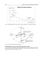
All state variables defining the current state of the model - and therefore the state of the
simulated power plant - should be located in the real-time data base (see Fig. 1). This 'data
base' is usually just a manageable piece of a shared memory. The exact (binary) copy of this
piece of memory can be used as a fully defined snapshot of the state.
After getting the proper command from the real-time executable the model programs
advance one time step and based on the previous state (the results of the previous step) they
calculate the state of the plant in the next step. Meanwhile, the actions of the operators in the
Control room are scanned by the man-machine interface (MMI programs) asynchronously
with a much shorter time step. The actions are stored in the I/O data base and are used by
the model programs.
If the time step is short enough (e.g. 0.2 sec or less) then the model programs can use only
one copy of the state variables. Before the actual step it contains data belonging to the last
step. During the execution of the model programs the state variables are calculated for the
next step one by one, and after the execution they all belong to the next step. Frankly
speaking, it is not exactly correct that some model programs should use data form the

Simulation and Simulators for Nuclear Power Generation

7
previous and the next step simultaneously, but if the time step is small enough - and it is -
then this fact cannot cause big errors.

State variables:
results of the
previous step
State variables:
describing the
actual state
Binary copy
to hard disk:
snapshot
Programs of
mathematical
models
I/O Data
base
MM Interface
programs e.g.
Control Room
interface
MMI
devices
(meters,
actuators)
Simulator programs
The Real-Time Data base

Fig. 1. Simulator programs and data storage

Control Room Interface
Operators
Archive

FREEZE
REPLAYRUN
Plots ,
Logs
Load Initial
Conditions,
Backtracks
Snapshots
Log of
Actions
EXIT

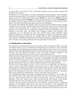
Fig. 2. States of the training simulator

Nuclear Power - System Simulations and Operation

8
If we decide to use this approach - having only one copy of state variables in the memory; it
is quite common in simulators - then we have to consider not to allow access to these state
variables until the actual act of integration is not finished. Accessing the state variables any
time means that other programs may fetch values not belonging to the same time instance.
For analogue values it is not a big problem, but solving logical circuitry it can lead to
confusion and incorrectness.
The different states of the simulator are presented on Fig. 2. Black arrows are state
transitions, white arrows symbolize data flow.
After starting up the simulator and all related programs (from the EXIT state) we reach the
FREEZE state. All programs are able to run, but practically neither of them is actually
running.
During the FREEZE state we are able to initialize the simulator, either loading in a saved
Initial Condition, or a previously saved snapshot (loading it is often called backtracking).

Adjusting switches in the Control room to the actual loaded state may become necessary; it
is done using the Control room set-up report made by the CR I/O system.
From the FREEZE state we can move to the RUN state.
The model programs calculate cyclically the actual state every time step and all the analogue
meters and annunciators of the Control room are driven accordingly. All the operations of
the staff are scanned in and stored in the Log of actions, and are added to the Archive,
together with the history of the most important parameters - there are several hundreds of
them. After the simulation session is finished, different logs and plots can be generated for
evaluation of the trainees.
During the simulation snapshots are taken regularly, or at any instant if the Instructor of the
actual simulation session commands to do so. Any time the instructor can stop the
simulation and return to the FREEZE state. During FREEZE state the parameters are
displayed in the Control room, and the situation can be analyzed. No operations can be
performed, though.
From the FREEZE state we can re-play how the operations happened earlier in the control
room. Backtracking using a snapshot, made earlier, we can enter the REPLAY state. During
the REPLAY state all the simulation is performed and the control room is driven as during
the RUN state, with the exception that no actions are accepted from the operators.
All operations are taken from the Log of actions, with their time stamps together, therefore
the trainees are able to follow what and how it happened earlier in the Control room.
Any time the REPLAY can be stopped, the state turns to the FREEZE state, and real
operations can commence entering the RUN state again. This is a very useful ability for the
Instructor, to go back in time, to show when and how a mistake was done, what are the
consequences and how it should be continued in a correct way.
4.2 Architecture of the simulators
Practically the full-scope replica simulator consists of the following parts:
• Computer system of the simulator. It incorporates the model programs, the simulation
control programs, the loggers, plotters, the archive etc. necessary to conduct a
simulation session.
• Control room and interface devices - a replica of the real control room equipped with all

meters, switches, pushbuttons, screens, memo-schema etc. and the hardware/software
devices (the MMI, the man-machine interface) enabling the computer system of the
simulator to handle them quickly and correctly.

Simulation and Simulators for Nuclear Power Generation

9
• Instrumentation and control devices taken from the real power plant. It is very
advantageous if we can take over the plant computer system, the core surveillance
system and other systems directly from the plant.
• The Instructor's system, the basic tool of the Instructors to control the simulation
session. The Instructor's system is usually hidden from the trainees, but sometimes,
when the Instructor is present in the Control room, he/she can use a remote control
unit to activate different pre-programmed events.
It is obvious that it is much better to use the real plant computer, the real core surveillance
system instead of simulating them. The operators feel the real controls; the real functions of
these units can be studied. The problem lies in the simulator functions to which these real
instruments are poorly suited. No real plant computer etc. is prepared to the stopped and
standing time, or even worse: to the backtracking, going back in time. It is difficult to
accommodate the real equipment to the new initial condition loaded into the simulator (e.g.
nominal state immediately after the cold shutdown state). It is obvious that all functions
somehow connected to the time (logging, making archives, and plotting) should be
excluded if possible. If they cannot be excluded: we have to refuse to integrate the real units,
we have to model their functions.
That is the main reason that all time-related functions are incorporated to the Instructor's
system: logging, plotting, making archives etc. etc. On the other hand, all simulator-specific
functions are evaluated in the simulator.


Fig. 3. The replica control room of the Paks NPPs training simulator

The most important function is the pre-programming of the malfunctions. All valves can
leak, all pipes can break, all pumps can be tripped, and there are very many equipment-

Nuclear Power - System Simulations and Operation

10
specific malfunctions. They can be activated promptly, or at a given time instance, and/or
when a logical function becomes 'true' (e.g. IF the temperature is higher than AND the
flow is less than etc.)


Fig. 4. The instructor's workstation of the Paks NPPs training simulator
4.3 Protection system refurbishment using simulator
The existing nuclear power plants were licensed earlier usually for 30 years; most of these
licenses expire in the next decade. Nowadays it is a common practice to prolong the
operation of the NPPs up to 50-60 years.
After the Chernobyl accident in 1986 requirements to the safety of nuclear power generation
units has been changed dramatically. As a result, many enhancements have been introduced
not only to the Instrumentation & Control (I&C) and Protections circuitry but to the
technological systems as well. Practically all these changes have been introduced on the
simulators first, in order to show the results of the forthcoming changes.
Even without that the “moral” and practical lifetime of the I&C systems is much less than
50-60 years, let say only 8-10 years. If they contain computers (and nowadays they do) this
becomes even shorter, about 5-7 years. The “aging” IT systems cannot be kept running for a
longer time. Spare parts and even software drivers become obsolete.
Replacing protection and control systems is relatively easy if the functionality remains the
same. Fig. 5. shows how it can be done.
First, while the old system is still in charge, the new system is placed parallel to it. Both
controllers (or others, as protections, interlocks) get the same inputs. The new controller
should be tuned until the response becomes the same in rather different situations, too. Then

the old controller can be replaced. This method cannot be used when it is dangerous or just
it is not allowed to test the equipment in extreme conditions. It is a rather new practice to
use simulators for I&C or other system’s refurbishments (Janosy, 2007 March). First the
simulators are used during the design of the new systems (Janosy, 2008). Integrating
software models of the newly designed models into the simulator in an interchangeable way
the proposed functionalities can be tested in normal, accidental and even extreme
circumstances (software-in-the-loop tests). After approval of the demonstrated functions


Simulation and Simulators for Nuclear Power Generation

11

Fig. 5. Old and new controllers tested in parallel
and performance, the manufacturing of the new hardware can be authorized. The new
hardware should be attached to the simulator, too, and the functionalities and the
performance can be compared with its already existing software model (hardware-in-the-
loop tests).
As it was mentioned before, it is not very easy to integrate real I&C hardware to the
simulator because of the special simulator functions of FREEZE, BACKTRACK, REPLAY.
This procedure had to be organized as it can be seen on Fig. 6.


Fig. 6. Instrumentation and control system (I&C) is tested on the training simulator

Nuclear Power - System Simulations and Operation

12
The black color indicates the original functions of the simulator. The technological models
advance in time using their state variables. The value of the measurements are calculated

and the old I&C models calculate the control parameters (e.g. control valve and rod
positions) governing the technological models. The development of the new system is made
in four consecutive steps.
1. The new controllers' mathematical models are constructed and their simulation models
are placed parallel with the old one (blue boxes). On the basis of the same
measurements the new model calculates the control parameters. In this phase the
(software) switch is placed to the (Guided) position, that means that the control actions
of the new controller are only logged, the old controller model is in charge.
2. If everything looks perfect, the switch is thrown into (Full) position, and the 'software in
the loop' mode is achieved.
3. After thorough testing the new controller is manufactured and using some temporary
I/O hardware interface (red boxes) it is connected to the simulator. (Spare parts of the
Control room I/O can be used). The new hardware is driven by the measurements, too,
but the new software governs the simulator - (SW) and (Full) position of the switches.
4. If according to the logged response of the hardware is OK, the upper switch can be
thrown to (HW) position. This is the 'hardware in the loop' mode of operation.
Thanks to the simulator, the new I&C equipment can be tested under extreme conditions,
too, without the slightest economic and environmental risks.
Practically everything can be tested before the plant stops. During the refueling - which
usually takes more than 20 but less than 30 days - the new equipment can be integrated to
the real unit and in the same time the idling operators can study the behavior of the new
I&C on the simulator in 'software in the loop' mode.
5. Nodalisation problems of the reactor models
The most important and difficult part of the simulation programs and the simulators is the
reactor model. Fuel elements, integrated into fuel assemblies produce heat in the nuclear
reactors in rather difficult, harsh conditions. The pressure and temperature is high - up to
160 bar and 320°C - and the power density in some reactors reaches 90 kW/liter and above.
They are made from expensive metals using expensive technologies. They should not leak -
the cladding represents the first barrier between the radio-active materials and the
environment (usually there are at least three barriers). If there is a remarkable leak, the

reactor should be stopped and the leaking fuel assembly replaced - a procedure causing
significant economic loss.
Nevertheless, some fuel assemblies are well made and they practically never leak. During
the 20-year-history of the four-unit Paks NPP there was detectable leak only once or twice.
The fuel elements originally spent three years in the core, nowadays they stay for four years
- with slightly higher uranium content, of course. If they should stay for five years, the
increasing of the enrichment is not enough - the control system of the reactor is not designed
to cover the excessive reactivity of the core, produced by the higher enrichment of the fresh
fuel.
The solution is the Gadolinium (Gd) which is a burnable neutron poison. In the first year -
or so - it helps to cover the excessive reactivity by absorption of neutrons, then it burns out
and do not causes any problem in the upcoming years. Now we replace at the Paks NPP
every year 1/4th of the fuel elements with fresh ones. If we start to replace them with the

Simulation and Simulators for Nuclear Power Generation

13
new types, supposed to stay for five years, it means that we are going to use mixed cores at
least for four years. These cores need special treatment and the operators should be trained
to it. The core surveillance system must be fitted to these mixed cores, too. To train the
operators to their more sophisticated duties we had to replace the reactor model and the
model of the primary circuit with more elaborated 3D spatial models.
We have 349 fuel assemblies in the core; each of them can be of different age and different
composition. The core configuration is carefully optimized each year to ensure that the
power distribution and burn-out corresponds to the maximal safety and to the best fuel
economy. Careful design of the reactor loads results in negative temperature and volumetric
coefficients that means that the reactor is capable to self-regulate its power - because making
the coolant hotter and thinner means worse neutron balance and therefore it decreases
nuclear power.
These effects make the neutron kinetic model of the reactor and the thermo-hydraulic model

of the primary cooling circuit tightly coupled; therefore they mathematical models must be
solved simultaneously. Describing very different physical phenomena we get very different
equations - that leads to severe problems of the simultaneous numerical solution. (Hazi,
Kereszturi et al., 2002)
The crucial point is: how to nodalise the nuclear reactor and the primary circuit in order to
achieve high fidelity of simulation with reasonable computer loads - in other words
achieving accurate simulation and still remaining in real-time. It looks easy to divide the
equipment to very small parts, and solve the problem using them as coupled nodes.
Decreasing the size of the individual nodes not only increases their number according to the
third power, but in the same time it significantly decreases the necessary time step of the
numerical integration.
5.1 Nodalisation problems: Neutronics
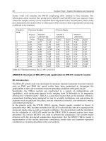
As it is shown on Fig. 7, we have in the core 349 hexagonal fuel assemblies (the numbers
outside the core refer to the six cooling loops). The 37 numbered fuel assemblies are used to
control the chain reaction. They are twice as long as a normal fuel assembly. The upper part
is made from special steel designed do absorb the proper amount of neutrons in order to be
able to control the chain reaction. The lower part is a usual fuel assembly containing usual
amount of fuel. Pulling out this control assembly means that the lower part enters the core,
lowering it causes this part to leave and to be replaced by the neutron absorber assembly.
The 37 control assemblies are organized into 6 groups, containing 6 assemblies except the
6th one, which contains 7 (this 7th is the central one). The first five groups with 30
assemblies are used as the "safety rods", fully pulled out during normal operation and fully
lowered during reactor shut-down. The 6th group is normally used as "control rods", during
normal operation they are always in different intermediate positions according to the
prescribed power of the reactor. In some very rare situations the 5th group is helping to the
6th one, sometimes staying in intermediate position, too.
That evidently means that the first four groups do not influence the spatial distribution of
the neutrons, their absorbents are pulled out and their fuel assemblies are inserted.
Lowering them the reactor is shut down and the spatial distribution is not interesting any
more. In the same time, the last two groups - the 5th and the 6th - can seriously influence the

3D distribution of the neutrons, being in different intermediate positions according to the
different operating conditions of the reactor and the primary circuit.

Nuclear Power - System Simulations and Operation

14
The nodalisation of the core from the neutron kinetics point of view does not leave us too
much freedom: each "neighbor" to each assembly can be of different "age" in the reactor
(zero to four, later zero to five years), with or without Gadolinium content accordingly.
Different "age" means different burn up, thus different stage of enrichment and different
isotope content. That means that in horizontal plane each assembly should be a separate node.
As to the vertical nodalisation, we must have not less than 8 or 10 planes to get enough
resolution (8 to 10 points) to describe the axial neutron (and heat) distribution. We have
chosen 10 planes vertically - that means, we have finally 349 x 10 nodes for the KIKO3D
model (Kereszturi et al., 2003).
Real-time spatial (3D) simulation of 3490 nodes in several groups of neutrons according to
their actual energy requires huge computer power. The only way to do it using several
processors; it means to separate the time and space problem. The result can be written as a
product of two functions: the amplitude function of time and the distribution function of
space. Solving the equations in different processors means that these programs have access
to the data of the other only after finishing the actual time step, and this means that delays
are introduced.


Fig. 7. The map of the core with the 349 fuel assemblies, including the 37 control ones
5.2 Nodalisation problems: Thermo-hydraulics
Thermo-hydraulic nodes should be much larger in space than the neutron-kinetic nodes. It
is connected with the 0.2 sec. time step of the full scope replica simulator of the power plant.
If we want to avoid large number of iterations, the amount of the steam/water
leaving/entering the node each time step must be probably less than the full amount of the

steam/water inside the node. It means that if we multiply the maximal feasible volumetric
flow-rates with the 0.2 sec. integration time step, we get the minimal volumes for the nodes
in question.

Simulation and Simulators for Nuclear Power Generation

15
Fig. 7. shows the thermo-hydraulic nodalisation of the reactor as well. According to the
reasons explained above, we have much less thermo-hydraulic nodes radially in the core,
and the number of the axial layers is only half that of the number of neutronic nodes: we are
limited here to only five layers. The reactor core is divided radially to only six outer, six
inner and one central node: altogether 13 nodes.
Each of the outer six nodes marked with different colors consists of 40 fuel assemblies. The
inner six nodes - all are marked as green - contain 16 fuel assemblies each but one of them
belongs to the 5
th
control rod group, one of the to the 6
th
control rod group. The 13
th
, the
innermost small node contains 13 fuel assemblies, one of them - the central - contains the 7
th

rod of the 6
th
group.


Fig. 8. Debugging tool for the core nodalisation and for the six cooling loops

Nuclear Power - System Simulations and Operation

16
This kind of thermo-hydraulic nodalisation provides the following benefits:
• During operation on power, only control rods of the 5
th
and 6
th
control rod group may
have intermediate positions, influencing the spatial distribution of the neutrons. The
inner 6 nodes and the central node are responsible for the calculation of these effects.
• One or more cooling loops may fail, usually because of the tripped main circulating
pumps (MCPs). The six outer large nodes can respond spatially to these effects.
The thermo-hydraulic model has to deal not only with the reactor vessel but the six cooling
loops of the primary circuit.
The original instrumentation of the nuclear power plant can not show the power, the
pressure, the temperature and the steam content of the water in each simulation node of our
simulator. It is not necessary to measure these parameters in such detail for the operation of
the plant. It means that the full-scope replica simulator has no tools to follow the actual
values in these nodes. For development and debugging we had to develop special
debugging tools (programs) to display these data on different windows on the screen in
order to follow the performance of our model programs closely (see Fig. 8).
Thanks to the nodalisation scheme described above, different spatial effects in the core can
be studied. As an example, the "rod drop" malfunction is presented.
If a control rod erroneously drops into the core, the negative reactivity caused by it can be
compensated by the power controller, pulling all the other rods a little out from the core.
However, the power locally will be less around the fallen neutron absorber.
All well-designed reactors are self-regulating, that means overheating causes negative
reactivity thus decreases the heat power, and overcooling does the opposite - it leads to

positive reactivity and the power increases a little. This effect compensates the locally
introduced (by the fallen rod) negative reactivity, and that's why the distortion of the power
field - and the resulting temperature field - is not so strong than it could have been expected,
not taking into account the temperature effects and the resulting self-regulating features.
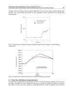
However, the resulting asymmetry of the temperature field is remarkable, as it can be seen
on Fig. 9.
5.3 Reactor thermo-hydraulics
Normally the primary circuit of a pressurized water reactor is filled up with water and there
is no boiling. Nevertheless, we have the pressurizer with the steam cushion, the secondary
parts of the steam generators with boiling, the steam headers, therefore we have to construct
a two-phase-flow (steam, water) model anyway.
Moreover, in case of LOCA (Loss of Coolant Accident) if the water flows out through the
break of some pipelines, the emergency core cooling circuits step in, pump water into the
primary circuit and the reactor vessel in order to keep the core covered with water and
cooled. Air and other non-condensable gases may enter the primary circuit. During the
startup of the plant the initial pressure is reached by nitrogen cushion in the pressurizer.
Because these states the simulation model should handle not only water and steam, but non-
condensable gases (third component.)
The best tool to simulate these states is the so called "6 equation" model - energy, mass and
momentum balance equations for steam and water separately, but with enabled state
changes (boiling, condensation). (The non-condensable gases usually are added to the steam
phase but state changes are disabled for them).
Solving 6-equation models in real time is an exceptionally demanding task, requiring very
powerful computers. Things are getting much simpler using 5 equation models (common


Simulation and Simulators for Nuclear Power Generation

17

Fig. 9. Picture of the in-core surveillance system VERONA - driven by "rod drop" state data
from the simulator
equation for the momentum of steam and water) but in this case the water and steam
velocity should be the same - these models are accurate only in case of low steam content
(emulsion flow). Higher steam content or stagnant flow causes phase separation and different
speeds. The commonly used solution is the so called "5½-equation" model - one momentum
equation but so called "drift flux model" which allows different speeds for water and steam
but handles them with algebraic approximations. The RETINA code (Reactor Thermo-
Hydraulics Interactive) can solve both the 6 and the 5½ equation systems (Hazi et al, 2001)
The most demanding task during the tuning and V&V of the simulator is to tailor these
drift-flux correlations to behave correctly in very different circumstances - stagnant, layered
coolant in the pressurizer vessel, isolated loop, etc
We have very different situations - normal operating and transients, stopping, cooling
down, heating up, reaching criticality of the reactor, loading up, and separating loops with
main gate valves (a rare feature possible only for Soviet/Russian reactors). There real art
during the V&V of the models lies in handling and tuning of the drift flux correlations
(nodes above each other, separating, nodes horizontally following each others, pipes and
stagnant coolants in vessels, etc.)
As non-condensable gases are carried with steam, boron acid solvent (used to absorb
neutrons) and radio-nuclides carried with water (in case of leakage) are simulated, too, but

Nuclear Power - System Simulations and Operation

18
this task is much simpler than the correct simulation of the two-phase-flow. (However,
"aging", decaying radio-nuclides continuously are changing the concentration of different
isotopes and this has to be taken into account, too.)
The simulation of the normal operating modes of the power plant are the less demanding
for the stability of the numerical integration of the models, and in the same time we have
ample data and recordings to fit the parameters of our models. On the other hand, the

training of the operators to anticipated (but rarely happening) transients and accidents is the
most important and valuable, but these are difficult physical states with no data (so far, so
good) to verify and validate the simulation.
The scope of simulation - by definition of the full-scope, replica simulators - covers anything
that can happen to the filled-up primary circuit with the closed reactor vessel. (Up to now
we do not simulate open reactor vessel with interrupted circulation, as it is usual during the
refueling outage.)
Covering only the events happening to the hermetically closed primary circuit (with pipe
breaks and loss of coolant accident of course) that means:
• normal operation with normal transients (load changes, frequency regulation)
• bringing to power (heating up, reaching criticality with the reactor, producing steam,
speeding and heating up the turbines, reaching the nominal power
• stopping the reactor, cooling down, changing to natural circulation without the pumps,
etc.
• malfunctions of any kind, pump trips, valve jams, valve leaks, short circuits, failures of
electrical supplies, island mode of operation (separation from the electrical grid)
• accidents up to the design basis accident, which means a large-break LOCA - breaking
of the pipe of the pipeline of the main cooling loop.
According to the integration of the models described above, all these transients can be
studied in "4D" in the reactor - that means in time and space, too.
6. Conclusions
Simulation is not a profession: it is a way of life - I was told on my first international conference I
participated - 'Simulation 1977' in Montreaux, Swiss. I can add to that after 34 years: it is a
way of thinking, too. The first Reference shows the first book I had to study after I started
with simulation in 1970 (Ralston, 1965).
My greatest mentor, Assoc. Prof. Dr. Richard Zobel retired, and went out to his garden with
a pint of beer. The next day he started to model and simulate the sounds produced by the
small plashing waterfall in the corner of his garden, with great success, resulting in excellent
papers. After being invited later as Assoc. Professor in the Prince of Songkla University, Hat
Yai and Phuket Campuses, Thailand, where he survived the big tsunami in the Indian

Ocean on 2004, he became one of the leading experts in tsunami simulation. Dr. Zobel is
going definitely to model and simulate things up to the last minute of his life.
At the beginning the simulation was very different from the simulation we are making
today. We had no powerful digital computers available that time or they were used for
different purposes secretly - ordinary scientists had no access to them. We used sometimes
analogue computers with integrators made from operational amplifiers. Sometimes they
were not electrical, but pneumatic 'operational amplifiers'. Modeling meant not always
mathematical modeling - we had to use e.g. electrical analogy, representing long pipelines
by inductance, vessels and tanks by electrical capacity; pressure meant voltage and flow was
represented by electrical current.