Novel Applications of the UWB Technologies Part 11 potx

The Future of Ultra Wideband Systems in Medicine: Orthopedic Surgical Navigation
287




Fig. 15. Wireless insulin pump manager (Omnipod (n.d)).




Fig. 16. Wireless alcoholmeter (Alcosystem (n.d)).




Fig. 17. Capsule Endoscopy (Public Domain (n.d)).
Apart from ambulatory and personal medical devices, wireless surgical tracking devices
have also been developed to improve the accuracy and efficiency of diagnosis and surgery.
Image guidance surgical navigation system uses optical and electromagnetic trackers to
track the surgical instruments in the attempt to minimize the human error during surgery.
Optical system (Figure 18), uses two infrared cameras to triangulate the position of the
target instrument. Figure 19 shows an electromagnetic tracking device developed by
Ascension and GE healthcare. The system provides real time feedback of the current
position of the biopsy needle, as well as the needle path projection.

Novel Applications of the UWB Technologies
288

Fig. 18. Optical tracking devices for surgical navigation (Metronics).



Fig. 19. The biopsy needle is coupled with electromagnetic tracking device to provide
feedback of the needle positions (Ascension), (G.E. Healthcare).
2.2 Current research
The commercially available devices mentioned in previous section have undergone many
years of research and development. The following section is going to look at some of the
current researches being done with wireless medical device.
While there are many wireless ambulatory monitoring systems mentioned above, most of
them operate in a standalone mode with its own receiver. It would be more beneficial to the
physicians and health care professional to centralize all the information into one single
device. Tia Gao et al. introduced a wireless sensor network (WSN) system for medical
devices. (Gao, et al., 2008) The information from the sensors is wirelessly transmitted to the
server, and it can be accessed through handheld devices and computers (Figure 20). The
authors tested the system along with medical professions in a mock emergency situation
with satisfying results. Another focus of the research is to develop applications from the
sensor technologies. Pekka Iso-Ketola et al. developed a wireless medical device using an
accelerometer to monitor patient’s posture after total hip replacement (THR) surgery (Figure
21). (Iso-Ketola et al., 2008) The devices are also given to the patient such that they can
monitor and follow the precautions given by the surgeons.

The Future of Ultra Wideband Systems in Medicine: Orthopedic Surgical Navigation
289

Fig. 20. Patients' conditions are being monitored through a hand held device (Gao, et al.,
2008).

Fig. 21. Wireless hip posture monitoring system (Iso-Ketola, Karinsalo, & Vanhala, 2008).
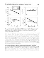
Shyamal Patel et al. developed a network of wireless acceleration sensing nodes that are
attached to different sections of the patient’s body as shown in Figure 22 (Patel, et al., 2009).
The data collected were analyzed. The calculated parameter can help with the diagnosis of
the severity of Parkinson’s disease. Stacy Bamberg et al. developed a wireless gait analysis
system. A force measuring system is placed within a shoe, and a triaxial accelerometers and
gyroscopes attached on the outside of the shoes as shown in Figure 23. (Morris & Paradiso,
2002) The sensors measure the forces and motion on the foot during gait.


Fig. 22. A network of wireless sensing nodes consists of accelerometers (Patel, et al., 2009).

Novel Applications of the UWB Technologies
290

Fig. 23. Wireless gait analysis system (Morris & Paradiso, 2002).
Aside from the patient monitoring and diagnostic tool, several research groups have been
concentrated on implantable medical devices. The technology to design and fabricate micro-
electromechanical system (MEMS) sensors and application specific integrated circuit (ASIC)
enables embedded measuring systems to be made in an extremely compact fashion. It is
now possible to measure in-vivo condition that was once impossible. Graichen Friedmar et
al. developed a complete embedded system to measure strain within a Humerus implant
(Figure 24) (Graichen et al., 2007). Antonius Rohlmann et al. also completed an embedded
system to measure the post operative load of spiral implants wirelessly as shown in Figure
25 (Rohlmann et al., 2007). D’Lima and Colwell modified existing knee implants with four
load sensors to measure the in-vivo stress on the implant after the total knee arthoplasty
(Figure 26) (D'Lima et al., 2005). Chun-Hao Chen et al. designed a wireless Bio-MEMS
system to measure the C-reactive proteins as shown in Figure 27 (Chen, et al., 2009).

Fig. 24. Telemetry strain measuring Humerus implant (Graichen et al., 2007).

The Future of Ultra Wideband Systems in Medicine: Orthopedic Surgical Navigation
291

Fig. 25. Wireless load measuring system for vertebral body replacement (Rohlmann et al.,
2007)


Fig. 26. Telemetry stress measuring knee implants (D'Lima et al., 2005).


Fig. 27. Wireless Protein detection with BioMEMS (Chen, et al., 2009)

Novel Applications of the UWB Technologies
292
Measuring the forces and contact areas in vivo is extremely valuable to researchers, implant
designers, clinicians, and patients. Measuring these values post operatively allows for
evaluation of the performance of current designs and prediction of future design
performance. Data on the in vivo load state of joint replacement components is required to
understand the structural environment and wear characteristics of that component. Normal
loads, load center, contact area, and the rate of loading need to be measured in order to fully
understand the kinematics and kinetics of the orthopedic implant. This data can be used to
help patients by allowing clinician to monitor implant kinematics, wear, and function. In the
cases of predicted premature wear, preventative measures such as orthotics, bracing, or
physical therapy could be used to avert the need for revision procedures. Additionally, one
of the major postoperative concerns was inflection. Currently, there is no effective way to
prevent it until symptoms are developed. Biosensing devices that react to disease related
protein can monitor and alert physicians to administrate antibiotic during early stage of the

infection.
3. Wireless signal propagation in hospital environments
The main concern with using wireless tracking and communication technology in the
operating room (OR) and other hospital environments is the high level of scatterers and
corresponding multipath interference experienced when transmitting wireless signals.
While the experiment from Clarke et al. provides quantitative data on how wireless real-
time positioning systems perform in the OR, it is also useful to look into narrowband and
UWB channels and their effect on narrowband and UWB signals for communication and
positioning applications (Clarke & Park, 2006). There are two typical approaches used when
modeling wireless channels: the first is statistical models used to model generic
environments (e.g. industrial, residential, commercial, etc.), which incorporate LOS or non-
line-of-sight (NLOS) measurements taken in the time and frequency domains, which are
then used in setting the parameters of these statistical models. The second method uses ray
tracing techniques to model specific geometrical layouts (e.g. buildings, cities) and can
provide a more accurate depiction of which obstacles and structures will have the greatest
effect on wireless propagation. The drawback with ray tracing is the static nature of the
results (i.e. results are only valid for a certain scenario of objects placed in the scene). Even if
the wireless systems in the operating room are static, other objects will not be including
people, patients, the operating table, and medical equipment.
3.1 Channel modelling in the operating room
A useful technique for modeling the operating room channel is to take time domain and
frequency domain measurements in the operating room. This can be done both during
surgery (live) and not during surgery (non-live) with variable Tx-Rx distances (e.g. 0.5 m to
4 m). Figure 28 and Figure 29 show the time domain and frequency domain setups to collect
data in the OR. Figure 30 and Figure 31 show the live and non-live setups where the layout
of the dual OR is shown to highlight the Tx and Rx locations for both the live and non-live
experiments. Note that both monopole and single element Vivaldi antennas are used for
transmission and reception. The basic strategy in the time domain is to send out a narrow
UWB pulse, either baseband or modulated by a carrier signal, in the 3.1-10.6 GHz band
approved by the FCC. Indoor measurements can also be measured at bands higher than the

standard 3.1- 10.6 GHz (e.g. 22-29 GHz) with the understanding that the effective isotropic

The Future of Ultra Wideband Systems in Medicine: Orthopedic Surgical Navigation
293
radiated power (EIRP) is limited to -51.3 dBm/MHz rather than the -41.3 dBm/MHz
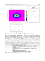
available in the lower band (FCC, 2002). Figure 32 shows the experimental setup during the
non-live case (Figure 31) for obtaining both time and frequency domain data while Figure 33
shows the experimental setup during an orthopedic surgery. When performing
measurements in the frequency domain, the typical approach is to use a vector network
analyzer to sweep across the UWB frequency range (e.g. 3.1 – 10.6 GHz) and measure the S-
parameter response of the channel where a UWB signal is passed between a transmitting
and receiving antenna. The inverse Fourier transform can then be used to convert the signal
from a frequency response into an impulse response in the time domain. This allows
frequency dependent fading and path loss as well as the RMS delay spread and power delay
profile measurements to be obtained. In Figure 29, a vector network analyzer is used to
collect data for frequency domain measurements.




Fig. 28. Experimental setup to collect time domain data in the operating room with the UWB
localization system (Mahfouz & Kuhn, 2011).




Fig. 29. Experimental setup to collect frequency domain data in the operating room for
characterization of the 3.1-10.6 GHz UWB band.
© 2011 IEEE

Novel Applications of the UWB Technologies
294




Fig. 30. Layout of dual operating room during surgery outlining the patient table, glass
walls, medical equipment, doors, and walls. The Tx and Rx were positioned 4 m apart
across the surgery (Mahfouz & Kuhn, 2011).




Fig. 31. Layout of dual operating room without surgery taking place where medical
equipment, glass walls, and the patient table have been removed. The Tx and Rx were
placed in the surgical area and moved from 0.5-4 m apart.




Fig. 32. Experimental setup in the operating room during non-live scenario (Mahfouz &
Kuhn, 2011).
© 2011 IEEE
© 2011 IEEE

The Future of Ultra Wideband Systems in Medicine: Orthopedic Surgical Navigation
295

Fig. 33. Experimental setup in the operating room during an orthopedic surgery.
3.2 Experimental results
Table 4 shows a truncated list of parameters for the LOS operating room environment fit to
the IEEE 802.15.4a channel model which were obtained with time domain and frequency
domain experimental data. Figure 34 shows the pathloss for the OR environment obtained
by fitting experimental data and compared to residential LOS, commercial LOS, and
industrial LOS. The pathloss in the OR is most similar to residential LOS, although this can
change depending on which instruments are placed near the transmitter and receiver or the
locations of the UWB tags and base stations in the room. Figure 35 shows pathloss obtained
for a Tx-Rx distance of 0.49 m where the transmitting (monopole) and receiving (Vivaldi)
antenna effects have been removed. Small scale fading effects can be seen as well as
frequency dependent pathloss, which is captured in the parameter κ in Table 4.

Figure 36 shows an example time domain signal where significant multipath interference is
caused by reflections from metal tables and walls. Figure 37 shows an example time domain
received signal for a Tx-Rx distance of 1.49 m using the monopole antenna for transmitting
and single element Vivaldi antenna for receiving. A decaying exponential is overlayed on
the received signal to highlight the intra-cluster decay, defined by γ
0
= 1.33 in Table 4. The
pathloss of the LOS OR channel is most like a residential LOS environment whereas the
power delay profile (PDP) is closer to an industrial LOS environment (γ
0
= 0.651) where
dense clusters of multipath quickly decay (rather than the residential LOS environment

where γ
0
= 12.53). The mean number of clusters (

=4) is in between the residential and
industrial LOS environments (


=3 and 

=4.75). The inter-cluster decay constant and
inter-cluster arrival rate (Λ and Γ) for the operating room channel are more similar to the
industrial LOS channel rather than the commercial or residential LOS channels. The
operating room LOS channel is similar to the industrial LOS channel in its time domain
characteristics (i.e. multipath interference and decay) while it is similar to the residential
LOS channel in its frequency domain characteristics.


Novel Applications of the UWB Technologies
296
Operating Room LOS
PL
0
[dB] -47.5
n
1.33
κ
0.95



4
Λ [1/ns] 0.095
λ [1/ns] n/a
γ
0
[ns] 1.33
k
γ
0.217
Γ [ns] 10.8
Table 4. Summary of parameters fit to IEEE 802.15.4a channel model with experimental
UWB data taken in the operating room (Mahfouz et al., 2009).


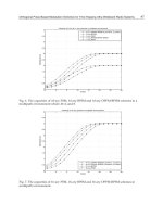
Fig. 34. Comparison of pathloss for IEEE 802.15.4a LOS channels. The pathloss for the OR
environment is most similar to residential LOS (Mahfouz et al., 2009).


Fig. 35. Pathloss obtained with the Tx and Rx placed 0.49 m apart where effects from the
transmitting (monopole) and receiving (Vivaldi) antennas have been removed. The
frequency dependence, κ, can clearly be seen as well as small scale fading effects (Mahfouz
et al., 2009).
01234
-65
-60
-55
-50
-45
-40
-35

-30
LOS Operating Room
LOS Residential CM1
LOS Commercial CM3
LOS Industrial CM7
Experimental Data Points
Pathloss (dB)
Distance (m)
46810
-70
-60
-50
-40
-30
-20
20 Sample Moving Average
Pathloss (dB)
Frequency (GHz)
© 2009 IEEE
© 2009 IEEE

The Future of Ultra Wideband Systems in Medicine: Orthopedic Surgical Navigation
297

Fig. 36. Experimental received time domain signal with noticeable multipath interference
caused by metal tables and walls in the operating room (Mahfouz & Kuhn, 2011).


Fig. 37. Example received signal in the time domain for a Tx-Rx distance of 1.49 m
highlighting the distortion (seen as expansion) in the LOS pulse due to a dense cluster of

multipath rays. The overlayed exponential is fit using γ
0
as outlined in Table 4 to show the
intra-cluster decay of the LOS cluster (Mahfouz et al., 2009).
3.3 Electromagnetic interference in the operating room
Electromagnetic interference (EMI) in the OR was measured across a wide frequency range
in the context of comparing the interference present in useable frequency bands for
narrowband and UWB communication and localization systems (for available bands see
Table 3).
3.3.1 OR indoor environment
EMI was measured over a large frequency band (200 MHz – 26 GHz) in the OR during four
separate orthopedic surgeries. Figure 38 shows the experimental setup in the OR. Besides
the operating table, numerous other pieces of medical equipment were present during the
surgery including an anesthesia machine, ventilator, surgical lamps, various monitoring
0 2 4 6 8 10 12 14
-10
0
10
20
30
40
Amplitude (mV)
Time (ns)
0481216
0
10
20
30
40
50

Expanded
LOS Pulse
where


=40.8 and


=1.33


e
-

k,l
/


Amplitude (mV)
Time (ns)
© 2011 IEEE
© 2009 IEEE

Novel Applications of the UWB Technologies
298
equipment, visualization screens, carts containing necessary orthopedic surgical tools, drills,
etc. Also, numerous people were present including the surgical team, orthopedic company
representatives, and spectators observing the surgery. The combination of people and
medical equipment closely packed into the OR creates a dense multipath indoor
environment that can greatly disrupt standard RFID tracking systems. UWB systems have

inherent advantages that make them a strong candidate for use in dense multipath
environments such as the OR.
3.3.1 Experimental setup
Various hardware was needed to get accurate measurements across the wide band of 200
MHz – 26 GHz. It should be noted that all reported gain and noise figure values are
averages across the frequency range of operation. Figure 39 shows the four antennas used to
cover the entire frequency range. The standard setup for each of the frequency bands
measured included an antenna, two stages of amplification, and a spectrum analyzer for
visualization. Commercial off-the-shelf components were used whenever possible. Table 3
lists the major medical, scientific, and UWB frequency bands in the US and Europe. A
majority of the scientific and medical bands in both Europe and the US fall between the
frequencies of 200 MHz – 3 GHz. Also, most RFID systems operate in the MHz range up to 3
GHz. Even though RFID systems can operate at 5.8 GHz or 24.125 GHz, limitations still exist
on how well a system with small bandwidth can handle the dense multipath environment of
the OR at these high frequencies. When looking at different wireless bands currently in use,
whether WLAN, cellular phones, GPS, or medical, the advantages of operating in the higher
frequency bands of 3.1 – 10.6 GHz and 22 – 29 GHz useable for UWB become clear.


Fig. 38. Experimental setup in the OR.
3.3.2 Experimental results
Electromagnetic interference was measured over the frequency range of 200 MHz – 26 GHz.
The results from these measurements can be seen in Figure 40-42. A number of signals were
detected in the lower frequency range of 400 MHz – 2.5 GHz. As shown in Figure 40, no
appreciable signals were picked up between 200 – 800 MHz. Although there is a small spike
near 470 MHz, it is only 6dB above the noise floor and is considered noise. Also, there are no
licensed frequency bands in the US that could correspond to the 470 MHz peak. Figure 41
shows the frequency band from 800 MHz – 3 GHz. A number of different signals were

The Future of Ultra Wideband Systems in Medicine: Orthopedic Surgical Navigation

299
found in this frequency range. The two strongest signals, which were found at 872 MHz and
928 MHz, correspond to CDMA2000 uplinks and downlinks. The peak at 1.95 GHz also
corresponds to a US cellular band. Finally, the peak at 2.4 GHz is caused by WLAN and
Bluetooth components. Figure 42 shows the frequency band from 3 – 26 GHz. No noticeable
signals were picked up across this entire band. This is somewhat unexpected since there are
ISM and WLAN bands between 5 – 6 GHz, which could be the major culprit causing
interference that could affect UWB systems.


Fig. 39. Antennas used in OR measurements: a) biconical, b) multiband disc, c) broadband
TEM horn, d) 4-element Vivaldi array (Mahfouz & Kuhn, 2011).


Fig. 40. Measured EMI over frequency range of 200 – 800 MHz (Mahfouz & Kuhn, 2011).
The frequency bands containing noticeable EMI correspond to widespread technologies that
will likely be seen in the average OR. One surprise was the almost complete absence of US
scientific and medical bands. Many medical devices do conduct wireless operations at the
frequency bands summarized in Table 3, but besides the WLAN signal at 2.4 GHz seen in
Figure 41, no significant EMI corresponding to these frequency bands was detected in the
OR. As outlined in Table 3, there is another UWB frequency band from 22 – 29 GHz that can
be used for localization systems. As seen from Figure 42, there is no EMI in the band from 22
– 26 GHz. One reason for having no EMI is that very few licensed bands exist between 22 –
29 GHz that would affect an OR. Also, signals in this frequency band tend to be attenuated
200 300 400 500 600 700 800
-60
-55
-50
-45
-40

-35
-30
-25
-20
Detected Power (dBm)
Frequency (MHz)
200 800 MHz
© 2011 IEEE

Novel Applications of the UWB Technologies
300
more by the atmosphere and are typically used for short range applications. Using UWB for
localization in the OR holds a distinct advantage over other technologies because of both the
large bandwidth used as well as the higher frequencies available for operation.


Fig. 41. Measured EMI over frequency range of 800 MHz – 3 GHz (Mahfouz & Kuhn, 2011).

510152025
-60
-55
-50
-45
-40
-35
-30
-25
-20
Detected Power (dBm)
Frequency (GHz)

3 26 GHz

Fig. 42. Measured EMI over frequency range of 3 – 26 GHz.
4. High accuracy positioning systems for indoor environment
Although UWB positioning systems are well established in their use for indoor applications
requiring 3-D real-time accuracy on the level of 10-15 cm, current commercial systems have
not been able to meet the stringent accuracy specifications (e.g. 1-2 mm or sub-mm 3-D) of
the next level of applications including smart medical instruments, surgical navigation, and
tracking in wireless body-area-networks.
4.1 Development of a high accuracy ultra-wideband positioning system
The challenges in developing a millimeter range accuracy real-time non-coherent UWB
positioning system include: generating ultra-wideband pulses, pulse dispersion due to
antennas, modeling of complex propagation channels with severe multipath effects, need for
extremely high sampling rates for digital processing, noise and sensitivity of the UWB
© 2011 IEEE

The Future of Ultra Wideband Systems in Medicine: Orthopedic Surgical Navigation
301
receiver, local oscillator phase noise (in the case of a carrier-based system), antenna phase
center variation, time scaling, jitter, and degradation due to overall system calibration. For
such a high precision system with mm or even sub-mm accuracy, all these effects should be
accounted for and minimized. The complete setup of the non-coherent UWB positioning
system is shown in Figure 43. The source of the non-coherent UWB positioning system is a
step-recovery diode (SRD) based pulse generator with a pulse width of 300 ps and
bandwidth of greater than 3 GHz. The Gaussian pulse is up-converted with an 8 GHz carrier
and then transmitted through an omni-directional monopole UWB antenna. Multiple base
stations are located at distinct positions to receive the modulated pulse signal. The received
modulated Gaussian pulse at each base station first goes through a directional Vivaldi
receiving antenna and then is amplified through a low noise amplifier (LNA) and
demodulated to obtain the I signal. Only one channel rather than I/Q is required since

energy detection and carrier offsets are also applied at the UWB receiver. After going
through a low pass filter (LPF), the I channel is sub-sampled using an UWB sub-sampling
mixer, extending the signal to a larger time scale while maintaining the same pulse shape
(Zhang et al., 2007). The PRF clocks are set to be 10 MHz with an offset frequency of 1-2 kHz
between the tag and base stations which corresponds to an equivalent sampling rate of 50-
100 GS/s. Finally, the extended I channel is processed by a conventional analog to digital
converter (ADC) and standard FPGA unit. Leading-edge detection is performed on the
FPGA. The time sample indices are sent to a computer where additional filtering and the
final time-difference-of-arrival (TDOA) steps are performed to localize the 3-D position of
the UWB tag.


Fig. 43. System architecture of non-coherent UWB positioning system which includes a
carrier-based transmitted signal at the tag and a combination of downconversion and
energy detection at the UWB receiver.
To detect narrow pulses on the order of a few hundred picoseconds (i.e. 300 ps or 3 GHz
bandwidth in our system), analog to digital converters with at least 6 GS/s are needed to
satisfy the Nyquist criterion. However, such high performance ADC units are currently

Novel Applications of the UWB Technologies
302
either not commercially available or too expensive for most applications. A realistic
alternative approach to real-time sampling is to sub-sample the UWB pulses while
maintaining the initial pulse shape through extended time techniques. The extended UWB
signals can then be handled by readily available commercial ADCs, reducing overall system
cost (Zhang et al., 2007).
The sampler utilizes a simple broadband balun structure and a
balanced topology.
The non-coherent architecture of the current UWB positioning system places stringent
requiremens on phase noise specifications of the local oscillators at the transmitter and

receiver. The use of a reference tag partially mitigates the local oscillator phase noise and
temperature effects at the UWB receivers. Even with a reference tag, the phase noise
presents a formidable challenge to achieving millimeter 3-D real-time accuracy. High phase
noise carriers (e.g. free running voltage controlled oscillators) cause up to an order of
magnitude (e.g. cm) greater error than low phase noise carriers. When attempting to achieve
millimeter and sub-mm accuracy, phase center variation of the antennas at the Tx/Rx is an
important source of error which needs to be taken into account. The transmitter employs a
UWB monopole antenna which provides an omni-directional radiation pattern with
minimal phase center variation while the receiver utilizes a single element Vivaldi antenna
for a radiation pattern directed at the view volume of interest. Noticeable variation of the
phase center is observed in both the E and H cuts especially for angles greater than ±30°.
High accuracy positioning systems must employ calibration techniques to remove the phase
center effects. For example, antennas used for GPS systems go through an advanced
automated calibration process which uses high precision robots to move the antennas to
6000-8000 distinct points in calibrating out phase center effects. More challenges appear in
achieving high accuracy real-time indoor positioning at the system-level. Cable length
effects at the UWB receivers must be accounted for and statically calibrated and removed
from the system. Time scaling effects due to system clock drift must be characterized and
calibrated out of the final TDOA calculations in a dynamic manner when moving around
the view volume. Time scaling effects change across the view volume due to the differences
in LOS ranges r
i
between the tag and each base station. The 3-D variation must be calibrated
out in order to get a highly accurate indoor positioning system achieving stable millimeter
range accuracy. Future improvements for this UWB indoor positioniong system include the
addition of real-time, multi-tag access (Kuhn et al., 2011) and utilizing comprehensive
simulation frameworks for accurate simulation of advanced mixed signal systems in
realistic indoor environments (Kuhn et al., 2010).
4.2 Real-time experimental results
Two 3-D experiments with unsynchronized LOs and PRF clock sources were carried out,

where a minimum of four base stations are needed for the 3-D measurements.
4.2.1 3-D dynamic free motion
Figure 44 shows a four base station setup where the 3-D positions were measured for each
base station utilizing the Optotrak 3020 system, which also serves as a reference for
comparing the 3-D real-time accuracy of our UWB localization system. The Optotrak 3020
has 3-D real-time accuracy of better than 0.3 mm. It should be noted that the spatial spread
of the base stations along the z-axis is the largest (2498 mm), while the x-axis is the smallest

The Future of Ultra Wideband Systems in Medicine: Orthopedic Surgical Navigation
303
(1375 mm). In the dynamic mode, the tag is moving randomly inside the 3-D space as shown
in Figure 44. The 3-D motion of the tag is then plotted and UWB measurements are
compared with Optotrak measurements. RMSE is used to report the error since it is the true
unbiased error when data values fluctuate above and below zero. Figure 45 plots the UWB
trace and Optotrak trace in the 3-D dynamic mode.
Figure 46 shows the 3-D dynamic errors in the x, y, and z axes over 1000 measured points.
The overall 3-D RMSE is 6.37 mm. The error along the x-axis contributed most to the overall
distance error, which can be explained by the limited spatial spread of base stations along
the x-axis and can be calculated using the PDOP definitions in (Mahfouz et al., 2008). Such
error can be mitigated through better arrangement of the base stations along the x-axis.



X
Y
BS2BS1
BS4
BS3
(-195, -610, -2083)
(554, 570, -1922)

(0, 753, -4420)
(1180, -1160, -4125)
unit: mm
Z
X
Space inside which tag
was moving around



Fig. 44. 3-D unsynchronized localization experiments, 4 base station distribution with
locations for each base station (Zhang et al., 2010).






Fig. 45. 3-D dynamic random mode with energy detection. UWB trace is compared to
Optotrak trace (Zhang et al., 2010).
© 2010 IEEE
© 2010 IEEE

Novel Applications of the UWB Technologies
304

Fig. 46. 3-D dynamic mode with energy detection.
x, y and z axes error compared to
Optotrak measurements (Zhang et al., 2010).
4.2.2 3-D robot tracking

The next non-coherent 3-D experiment is to dynamically track the robot position. The
monopole antenna and the reference Optotrak probe are tied together and fixed to the arm
of the CRS A465 robot. The robot arm set up is shown in Figure 47. Finally, the base stations
can be seen in Figure 48. The robot was pre-programmed to specifically cover 20 distinct
static positions in a 3-D volume, stopping for three seconds at each position and then
moving to the next position and so on. The measured traces by the UWB system are
compared to the Optotrak reference system as shown in Figure 49. Figure 50 shows the 20
distinct static positions taken by both the UWB and the Optotrak systems. The overall
dynamic 3-D robot tracking RMSE is 5.24 mm. In Table 5 the real-time non-coherent 3-D
experimental results are summarized under various scenarios. The reported RMSE are
based on 1000 continuous data points recorded and compared to the Optotrak 3020 system,
which served as the real-time reference of our UWB localization system and provides a 3-D
accuracy of better than 0.3 mm.






Fig. 47. Robot arm with UWB monopole and optical tracker attached (Mahfouz et al., 2009).
© 2010 IEEE
© 2009 IEEE

The Future of Ultra Wideband Systems in Medicine: Orthopedic Surgical Navigation
305


Fig. 48. Experimental setup outlining base station positions.

(a) 3-D view (b) XY plane


(c) XZ plane (d) YZ plane
Fig. 49. 3-D dynamic robot tracking. UWB trace compared to Optotrak trace: (a) 3-D view;
(b) XY plane; (c) XZ plane; (d) YZ plane (Zhang et al., 2010).
© 2010 IEEE

Novel Applications of the UWB Technologies
306

Fig. 50. 3-D robot tracking at static positions. UWB points compared to Optotrak points
(Zhang et al. 2010).

3-D Experiments RMSE (mm)
Tag free random motion 6.37
Robot dynamic tracking 5.24
Robot static positions (20 distinct locations) 4.67
Static position w/ 106 times of average 1.98
Table 5. Error Summary – 3-D unsynchronized localization experiments (Zhang et al. 2010).
5. Wireless MEMS sensors used as feedback control in an orthopedic
surgical navigation system
Over the past decade, orthopedic companies have been trying different methods and
protocols to eliminate one of the primary causes of implant failure in total knee
arthroplasty (TKA), which is the malalignment of the implants to the biomechanical axis
of the patient. To properly place the implant, the gaps after the resections between the
femur and tibia during extension and 90 degrees flexion have to be parallel to each other
and the gap size have to be the same (Figure 51). However, the surgeons are usually
working with a small incision with limited access to the joint. Moreover, the knee joint are
stabilized by the medial and lateral collateral ligaments. The laxity of the ligaments can

affect the gap balance.


Fig. 51. Flexion and Extension gap between the femur and tibia (To, 2007)
© 2010 IEEE
© 2007 IEEE

The Future of Ultra Wideband Systems in Medicine: Orthopedic Surgical Navigation
307
In order to help the surgeons to assess the tightness of the joint after resection, an
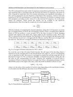
instrument was designed to provide quantitative feedback to the users. A wireless strain
measuring device was designed. The high level system design is shown in Figure 52. Two
types of sensors were investigated in the design of this instrument. The first type of sensor is
piezo-resistive based microcantilever as shown in Figure 53. When a piezo-resistive element
undergoes stress, the resulting strain causes changes in the resistance of the material. Hence,
it is possible to use to measure strain by monitoring the resistance of the material.


Fig. 52. High level design of a wireless strain measuring system (Qu et al., 2008)
The piezo-resistive microcantilevers here are used to measure a macro pressure that causes a
deflection in the microcantilever beam. The microcantilevers are tiny and extremely fragile. In
addition, silicon is not a FDA-approved biocompatible material unless specifically doped. This
specific application to measure macro forces requires a protective layer with a material that
damps the applied stress and provides a biocompatible interface for bodily contact. Medical
grade epoxy was used as a protective material for the sensors as well as providing a bio-
compatible surface to interface with the soft tissues. The epoxy was cured over the
microcantilevers to protect and to give a desirable force readout range. Curing procedures and
epoxy homogeneity were investigated to create the most reliable, non-interfering
encapsulation. Parameters investigated included viscosity, cure time, working time, heat cure,
and minimization of bubbles and microbubbles. EP30MED (Masterbond, Inc.) was chosen as

the most favorable epoxy for encapsulation. A microcantilever that was encapculated with a
2mm thick epoxy was used for mechanical testing as shown in Figure 54. An Instron 5544
testing machine was used. The properties of the encapsulated sensor are shown in Table 6.



Fig. 53. Piezo resistive microcantilever (Nascatec, Stuttgart, Germany) [To & Mahfouz, 2005]
© 2008 IEEE
© 2005 IEEE

Novel Applications of the UWB Technologies
308

Fig. 54. Microcantilever encapsulated in EP30MED epoxy.

Parameter Value
Range 0 – 300 kPa
Input 0 – 3.3V +/- 1%
Linearity 0.625mV/kPa (over range)
Repeatability 0.6444mV/kPa (over range)
Sensitivity 0.35455mV/kPa (over range)
Table 6. Properties of microcantilever encapsulated in 2mm of EP30MED (Qu et al., 2010)
The readout circuit for the microcantilever system was tested with off-the-shelf components
using an MSP430 (Texas Instrument) as microcontroller, ADG726 (Analog Device) as
multiplexer, INA331A2 (Texas instrument) as instrumental amplifier, and MAX1472/1473
as transmitter and receiver. The readout circuit is too bulky to be fitted inside a surgical
instrument. As a result, an application specific integrated circuit (ASIC) is designed
specifically for the reading of the microcantilever sensors. The ASIC includes the
multiplexer, signal conditioning circuit, analog to digital converter (ADC), and a buffer
interfacing with the transmitter. The footprint of the ASIC is shown in Figure 55. The

specification of the ASIC is shown in Table
7. The gain of the amplifier can be adjusted via
an external resistor. After examining the outputs of the microcantilever, the gain was
configured to 72. The overall system RSS error with microcantilever embedded within 2mm
thick of EP30MED is approximately +/- 1.79kPa.



Fig. 55. ASIC designed for microcantilever readout (Left: ASIC footprint, Right: ASIC with
testing package) (Qu et al., 2010)
© 2007 IEEE
© 2010 IEEE

The Future of Ultra Wideband Systems in Medicine: Orthopedic Surgical Navigation
309
Parameters Values
Analog input channels 16
Analog MUX switching frequency Oscillator dependent
A/D Converter input range ~ 200mV – 1589mV
A/D Converter resolution 8bit
A/D Converter rate 772 kHz
Band gap reference 1.249V
INA gain Gain resistor dependent
INA phase margin 65
o
INA Unit gain bandwidth ~ 2.4 GHz
A/D ENOB 7.24 bit
A/D SNDR 45.4 dB
A/D SFDR 56.4 dB
DNL +0.57/-0.42 LSB

INL +1.3/-0.2 LSB
Power supply 2.6 – 4.4V
Table 7. ASIC specification (Qu et al., 2010)
The final design of the instrument is designed to fit within a spacer block (Figure 56). The
spacer block is placed within the resection gap to identify the tightness of the joint.
Moreover, identifying the location of the high strain area can help the surgeons in balancing
the joint with appropriate ligaments release. The system design is separated into 3 layers.
An array of 30 microcantilever are arranged and wirebonded onto the circuit board. The
bottom most circuit board is the ASIC and the battery layer as shown in Figure 57. Two
switches are used to connect the poly Li
+
batteries to the electronics and sensors. Traditional
coin cell batteries are not suitable for this design as they are too large in size and they are
incapable of powering all 30 microcantilevers, which is about 70mA. The poly Li
+
batteries
can be made in customable shape and they are rechargeable. For the prototype, a USB socket
is used to recharge the batteries. High density sockets are used to connect the ASIC layer to
the sensors layer.


Fig. 56. Instrumented Spacer Block [To et al., 2006].
The middle layer is the TX PCB. The transmitter is using MAX1473 and configured the
carrier frequency to 433MHz. The material for the circuit board was changed to 0.0020”
rogers 4350 for better performance. A chipped antenna is used to further reduce the volume
© 2006 IEEE

Novel Applications of the UWB Technologies
310
required from traditional whipped antenna. The assembled PCB is shown in Figure 57. Each

side of the PCBs has 15 active sensing microcantilevers and 1 additional microcantilever for
reference on the left side of the PCB.


Fig. 57. Left: Top view of the signal processing layer; Center: Bottow view showing the
batteries; Right: Top view of assembled PCB (Right) with 15 microcantilevers arrayed on
each condyle. (Qu et al., 2008)
The second type of sensor being investigated was capacitive based MEMS device. Strain
sensing is accomplished by embedding pairs of electrodes with specific geometries in a
biocompatible material. Deformation of the embedding materials causes changes in the
configuration of the capacitor electrodes. However fabricating MEMS devices on polymeric
materials is not as straight forward as with silicon substrate. Researchers have shown that
polyimide can be used as a substrate material, and parylene can be used as the dielectric
material (1.5 m). It is noted that parylene has served as a substrate layer in early capacitve
fabrication when the sensor was left on the silicon wafer, but it poses a problem due to
adhesion and mechanical strength of the thin film during removal from the silicon substrate.
A negative-resist based photolithography fabrication was implemented to reduce time and
number of steps for fabrication. The electrodes consist of a 10 nanometer (nm) titanium
adhesion layer and 300 nm of gold deposited on the substrate via physical vapor deposition.
Array design is multi-faceted to understand the behavior of the sensors at a small scale and
to optimize design to boost readout speed, increase nominal capacitance, and decrease
crosstalk and parasitic effects specific to the configuration of this array. Increasing nominal
capacitance is most easily achieved through larger electrode size and thinner dielectric
layers, thus presenting a tradeoff between keeping sensor size to a minimum and nominal
© 2008 IEEE

The Future of Ultra Wideband Systems in Medicine: Orthopedic Surgical Navigation
311
capacitance at an appropriate level for accurate measurement. Similarly, the spacing needs
to be optimized between closeness (providing high spatial resolution across the array), and

crosstalk (sensors too close to one another affecting readout). A uniaxial and triaxial strain
measuring device was fabricated as shown in Figure 58.


Fig. 58. Capacitive based MEMS strain measuring device (Left: Uniaxial(Pritchard et al.,
2008), Right: Triaxial (Evans III, 2007)).
An array of sensors was tested using an MTS (Eden Prairie, MN) 858 Table Top System
mechanical testing machine with a 2.5 kN load cell. The load profile is shown in Figure 59. A
protective polyimide layer was placed over the electrodes and a second protective layer over
the entire assembly. Unlike the microcantilever sensors, no protective epoxy layer was
required. Similar to the piezoresistive microcantilever, a transition was made from using off-
the-shelf IC to ASIC electronics for the capacitive MEMS sensors. An ASIC consisting of
diode array, matched capacitor capacitance to voltage converter and a custom designed
instrumental amplifier as shown in Figure 60.


Fig. 59. Load profile for capacitance array test. Test is from 5 pF capacitor array (Evans III,
2007).
-1.50E-15
-1.00E-15
-5.00E-16
0.00E+00
5.00E-16
1.00E-15
1.50E-15
2.00E-15
2.50E-15
3.00E-15
3.50E-15
0 200 400 600 800 1000 1200 1400 1600 1800 2000

Time (sec)
Capacitance (pF)
-25
0
25
50
75
100
125
Load (kN)
Capacitance Load
© 2008 IEEE
© 2007 IEEE
© 2007 IEEE